Highly Interpretable Prediction Models for SNP Data

Robin Nunkesser

Hamm-Lippstadt University of Applied Sciences, Marker Allee 76–78, 59063 Hamm, Germany

Keywords:

Interpretable Machine Learning, SNP Data, Genetic Programming, Simulation Study.

Abstract:

Binary prediction models for SNP data are often used in genetic association studies. The models should

be highly interpretable to help understand possible underlying biological mechanisms. logicFS, GPAS, and

logicDT can yield highly interpretable prediction models. The automatic prevention of overﬁtting requires

improvement, however. We propose using GPAS as a black box and applying an external method for automatic

model selection. We present an approach using the GPAS algorithm as a black box and show initial results

on simulated data. The simulation is designed to motivate research to extend GPAS with automatic model

selection. Additionally, we give an outlook on further extensions of GPAS.

1 INTRODUCTION

Single Nucleotide Polymorphisms (SNPs) are the

most common type of genetic variation in humans.

Each SNP represents a difference in a single DNA

building block (nucleotide). For example, a SNP

may replace the nucleotide cytosine (C) with the nu-

cleotide thymine (T) in a certain stretch of DNA. The

human genome consists of approximately 3.2 billion

base pairs, however (International Human Genome

Sequencing Consortium, 2001). Typically, only the

variants occurring with a frequency of at least one

percent are considered. It is widely known that, in

the analysis of disease risks, it is important to not

only consider the effect of single SNPs, but that of in-

teractions with demographic and environmental data

or other genetic variables such as other SNPs (Garte,

2001; Che and Motsinger-Reif, 2013).

A high degree of interpretability in prediction

models is especially desirable, as such models may

also help to understand possible underlying biolog-

ical mechanisms. High interpretability is achieved,

for example, by logicFS (Schwender and Ickstadt,

2007) and GPAS (Nunkesser et al., 2007) (according

to Chen et al., 2011). In addition, newer approaches

such as logicDT (Lau et al., 2024) are speciﬁcally de-

signed to yield highly interpretable prediction mod-

els, while maintaining a high predictive ability. All

of the aforementioned approaches yield very good re-

sults on simulated and real data. However, the auto-

matic prevention of overﬁtting requires improvement.

Additionally, it is shown, that the approaches are ca-

pable of surpassing speciﬁc and more general state-

of-the-art algorithms chosen by Microsoft’s AutoML

for the considered problem. It is therefore of inter-

est to extend them to multi-valued responses or other

categorical predictors besides SNPs and to compare

these extensions to more general algorithms.

This position paper argues that the above men-

tioned possible improvements offer important oppor-

tunities for research and presents work in progress

on the automatic prevention of overﬁtting in GPAS

and an outlook on possible further extensions. In a

ﬁrst step, the relevance of the research is shown by a

short comparison of the methods logicFS, GPAS, and

logicDT with state-of-the-art machine learning algo-

rithms chosen by Microsoft’s AutoML on simulated

data. The simulation is intended to motivate research

to extend GPAS with automatic model selection. In a

second step, we present an approach using the GPAS

algorithm as a black box to extend GPAS with auto-

matic model selection. The approach is evaluated on

the same data as the comparison. In a third step, we

give an outlook on further extensions of GPAS.

The paper is structured as follows: Section 2 gives

an overview of related work. The following Section

3 gives a brief overview of SNP data and highly in-

terpretable prediction models. In Section 4, we will

provide a brief comparison of the methods logicFS,

GPAS, logicDT, and Microsoft’s AutoML by showing

results on simulated data. In Section 5, we present an

approach to extend GPAS with automatic model se-

lection, ﬁnishing in Sections 6 and 7 with future work

and conclusions.

Nunkesser, R.

Highly Interpretable Prediction Models for SNP Data.

DOI: 10.5220/0013137600003911

Paper published under CC license (CC BY-NC-ND 4.0)

In Proceedings of the 18th International Joint Conference on Biomedical Engineering Systems and Technologies (BIOSTEC 2025) - Volume 1, pages 555-562

ISBN: 978-989-758-731-3; ISSN: 2184-4305

555

2 RELATED WORK

With regard to the main topics of this paper (highly

interpretable prediction models for SNP data and au-

tomatic model selection for such models), the fol-

lowing related work must be mentioned: Lau et al.

(2024) proposes logicDT as designed to yield highly

interpretable prediction models with a high degree

of predictive ability. Nunkesser (2008) describes ap-

proaches for automatic model size selection in GPAS

which were not integrated into the available algo-

rithm. The work of Chen et al. (2011) offers a review

of methods for identifying SNP interactions which

also compares interpretability.

An overview of more general methods for SNP

data is given in Lau et al. (2024). These include

the following, as yet unmentioned, methods: tree-

based statistical learning methods such as decision

trees, random forests, or logic regression applied in

Bureau et al. (2005); Winham et al. (2012); Ruczinski

et al. (2004), for example. Tong et al. (2021) give an

overview of further methods for SNP data.

For an overview of principles in interpretable ma-

chine learning, we refer to Rudin et al. (2022).

3 BACKGROUND

In the following, we will give a brief overview of SNP

data and highly interpretable prediction models.

3.1 Single Nucleotide Polymorphisms

Less than 1% of human DNA differs between indi-

viduals. In absolute terms, these are still millions of

base pair positions at which different bases can occur.

Each of the forms a DNA segment can take is called

an allele. Alleles occurring in more than 1% of the

population are called polymorphisms. Looking at a

ﬁxed base pair position or locus, a polymorphism at

this speciﬁed locus is called a single nucleotide poly-

morphism. In an analysis concerning the genotype

of individuals, we consider the chromosome pairs of

an individual. A SNP typically has two alleles, the

major allele occurring in the majority of the popu-

lation and the minor allele (often denoted by A and

a). We consider diploid organisms with chromosome

pairs, therefore a SNP in our analysis can take three

forms: AA (homozygous reference), Aa/aA (heterozy-

gous variant), and aa (homozygous variant). In the

following, the SNP values are frequently encoded as

AA = 1,Aa/aA = 2,aa = 3 (another more popular en-

coding is AA = 0,Aa/aA = 1, aa = 2 which may also

be interpreted as the number of minor alleles).

3.2 Highly Interpretable Prediction

Models for SNP Data

Interpretability depends on the domain, but in general,

a model is interpretable if the reasoning processes are

more understandable to humans (Rudin et al., 2022).

The methods considered operate on genetic risk

factors given by SNPs and are an attempt to predict a

binary disease status. More precisely, in case-control

genetic association studies on SNP data, we intend

to understand a procedure that produces output in

{case,control} (encoded by B = {0,1}) from inputs

in {AA,aA/Aa,aa}

(encoded by P

= {1,2, 3}

= {0,1,2}

) where cases are individuals with the

considered disease and controls are individuals with-

out the considered disease.

logicFS and GPAS return boolean models repre-

senting a function

f : P

→ B

while logicDT and AutoML provide risk estimates

representing

f : P

→ [0,1] .

The models returned by logicFS, GPAS, and logicDT

are highly interpretable, as they are given in a form

that is easily understandable by humans. In addition,

they resemble the models in Garte (2001).

Garte (2001) states that it is "to be expected that no

single metabolic gene variant should ever be observed

to have a large role in cancer susceptibility for any

general cancer type" and that in "some cases, effects

were only observed in the presence of two or more

risk alleles." The presented studies in Garte (2001)

suggest models such as

a woman with alleles of GSTM1 and GSTT1

that is premenopausal and frequently drinks

alcohol or an african-american woman with an

allele of CYP1A1 or a woman with an allele

of NAT1*11 that frequently smokes

for an increased breast cancer risk. The methods con-

sidered rely on subgroups with similar demographic

and environmental data and therefore only consider

the SNPs. The methods are not restricted to SNPs,

however. logicFS, GPAS, and logicDT can also op-

erate on dichotomized data. According to Nunkesser

(2008) GPAS is extendable to general ordinal data.

From the results of preceding studies it seems rea-

sonable to assume that the models should not be very

large. Highly interpretable prediction models should

be similar to the models in Garte (2001). This would

also help to understand possible underlying biological

mechanisms.

BIOINFORMATICS 2025 - 16th International Conference on Bioinformatics Models, Methods and Algorithms

556

4 SHORT COMPARISON OF

RELEVANT METHODS

scrime (Schwender and Fritsch, 2018) is a popular R

package that is capable of simulating SNP data. With

standard parameters, the function simulateSNPglm

simulates case control data where the case risk is in-

creased by either SNP6 not being AA and SNP7 being

AA or SNP3, SNP9, and SNP10 all being AA. Alter-

natively, we can denote this with boolean operators as

follows (∧ may be omitted in monomials):

(SNP6 ̸= AA)(SNP7 = AA)

∨ (SNP3 = AA)(SNP9 = AA)(SNP10 = AA)

This data simulation corresponds to the observations

of Garte (2001) for subgroups with similar demo-

graphic and environmental data.

Please note that the following analysis may not be

as rigorous and fair as it should be. The main purpose

is to introduce the methods considered and to show

their relevance and potential for extensions. One

might think that the simulation from scrime may be

outdated by now, so we will also look brieﬂy at what

an analysis with state-of-the-art machine learning al-

gorithms chosen by Microsoft’s AutoML reveals. For

a future deeper analysis with simulated data, it it also

possible to use the more sophisticated simulations

based on scrime used in Lau et al. (2022).

4.1 Software Used

As mentioned above, we use the R package scrime

for data simulation. We use version 1.3.5 available

from CRAN. logicDT is also available from CRAN

and we use version 1.0.4. logicFS is available from

Bioconductor and we use version 2.24.0. GPAS is

part of the R package RFreak available from GitHub

and we use version 0.3-1. Microsoft’s AutoML is

part of ML.Net and we use version 16.18.2.

4.2 Microsoft AutoML

Figure 1 shows the accuracy (ratio of correctly pre-

dicted instances to the total number of instances) on

test data of the underlying model and the model cho-

sen by AutoML in 100 runs with standard parame-

ters for simulateSNPglm and AutoML. It is appar-

ent that the standard data simulated by scrime is still

complex enough for the comparison of different al-

gorithms. In addition, many of the machine learning

algorithms chosen by AutoML do not have compara-

ble interpretability to logicFS, GPAS, and logicDT.

Figure 1: Accuracy on test data of the underlying model and

the model chosen by AutoML.

!X5 & !X17 & !X95

!X5 & X57 & !X58

!X17 & !X19 & !X92

!X17 & !X19 & !X46

!X17 & !X19 & !X88 & !X92

X21 & X31 & !X59

X13 & !X47 & !X94

X13 & !X47

!X52 & X57 & X61

!X2 & X57 & X61

X57 & !X58 & X61

X57 & X61

!X5 & !X17 & !X19

X57 & X61 & !X92

X11 & !X13

0 2 4 6 8 10 12

Single Tree Measure

Importance

Figure 2: logicFS importance measures of interactions.

4.3 logicFS

For the purpose of demonstration, let us assume that

GPAS and logicDT are capable of automatically com-

puting the best model size. logicFS does not require

this assumption.

Figure 2 shows the importance measures of inter-

actions for an exemplary run of logicFS on the stan-

dard simulated data of scrime.

logicFS requires a recoding of the SNPs to be able

to handle the data. The ﬁve most important interac-

tions in Figure 2 are:

• (SNP6 ̸= AA)(SNP7 = AA)

• (SNP29 ̸= AA)(SNP31 ̸= AA)(SNP46 ̸= aa)

• (SNP3 = AA)(SNP9 = AA)(SNP10 = AA)

• (SNP29 ̸= AA)(SNP31 ̸= AA)

• (SNP29 ̸= AA)(SNP29 ̸= aa)(SNP31 ̸= AA)

Highly Interpretable Prediction Models for SNP Data

557

(SNP6!=1)

(255,142)

399 (45.54%)

(SNP9==1)

(336,227)

231 (26.36%)

(SNP7==1)

(177,56)

387 (96.99%)

(SNP10==1)

(214,104)

228 (98.7%)

(SNP3==1)

(144,41)

222 (97.36%)

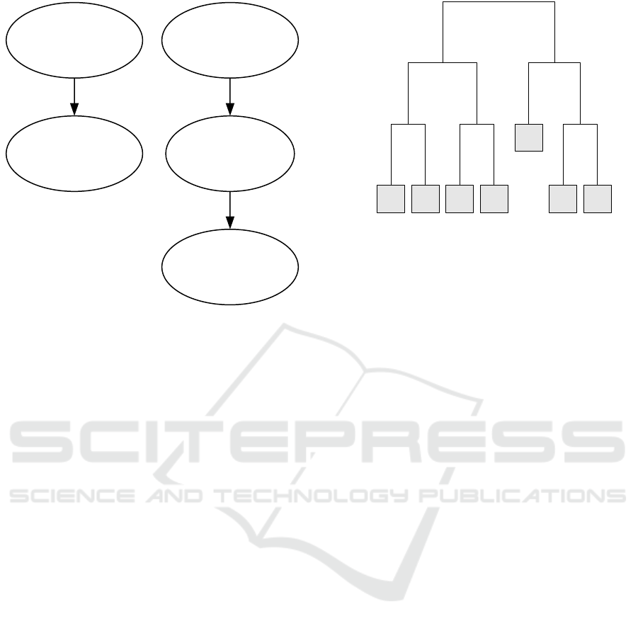
Figure 3: Exemplary returned interaction graph of GPAS-

Interactions.

The interactions of the underlying model are

found by logicFS. The model is highly interpretable,

but the interactions are provided in an isolated state

and there seems to be no way to distinguish

(SNP3 = AA)(SNP9 = AA)(SNP10 = AA)

from similarly important interactions.

4.4 GPAS

GPAS offers two different modes for the in-

tended purpose: GPASDiscrimination and

GPASInteractions. The former determines

(SNP6 ̸= 1)(SNP7 = 1)

∨ (SNP3 = 1)(SNP9 = 1)(SNP10 = 1)

as the best model with the same size as the true model,

which is in fact GPAS notation of the true model.

The latter returns a graph similar to the one in Figure

3. The graph shows as principal information for im-

portant alleles and interactions of alleles the number

of correct cases and false controls explained by the

corresponding interaction (in brackets; the ﬁrst value

needs to be maximized, the second minimized). We

have chosen a very strict pruning of subtrees for the

graph, showing only subtrees with frequencies above

75%.

With regard to the interpretability and precision

of the models, we can see that there cannot be a better

solution than the result of GPASDiscrimination for

simulated data, because the true model is found and

given in the biologically meaningful way described by

0.70 0.40 0.35 0.50

0.88

0.62 0.79

SNP10D

AND SNP9D

AND SNP3D

SNP31R

AND SNP6D

SNP3R

AND SNP7D SNP3R

AND SNP7D

SNP31R

AND SNP6D

SNP3R

AND SNP7D

0 =

= 1

0 =

= 1

0 =

= 1

0 =

= 1

0 =

= 1

0 =

= 1

Figure 4: Exemplary returned model of logicDT.

Garte (2001). The result of GPASInteractions is an

interesting and highly interpretable model which, in

this case, also shows the underlying model. We may

see more interactions with lower values for pruning,

however, making it an interesting alternative for real

data. An obvious extension would be to add to the

method strategies to prevent overﬁtting if no pruning

is applied.

4.5 logicDT

Figure 4 shows an exemplary returned model of log-

icDT. If we assign a case to probabilities > 0.5

and apply transformation rules, we get the following

model:

(SNP3 = AA)(SNP9 = AA)(SNP10 = AA)

∨ (SNP6 ̸= AA)(SNP7 = AA)

∨ (SNP3 = aa)(SNP31 = aa)

∨ (SNP6 ̸= AA)(SNP3 = aa)

∨ (SNP7 = AA)(SNP31 = aa)

The model is highly interpretable, as with logicFS,

but there does not seem to be a straightforward way

to distinguish (SNP6 ̸= AA)(SNP7 = AA) from simi-

larly important interactions.

4.6 Conclusion

If we assume that GPAS and logicDT are capable

of automatically computing the best model size, all

methods apart from AutoML are capable of ﬁnding

the underlying model (in the case of logicFS and log-

icDT with additional interactions). GPAS is capable

of ﬁnding the true model in the most interpretable

way. logicFS and logicDT are capable of ﬁnding the

true model, but in the cases considered here there

BIOINFORMATICS 2025 - 16th International Conference on Bioinformatics Models, Methods and Algorithms

558

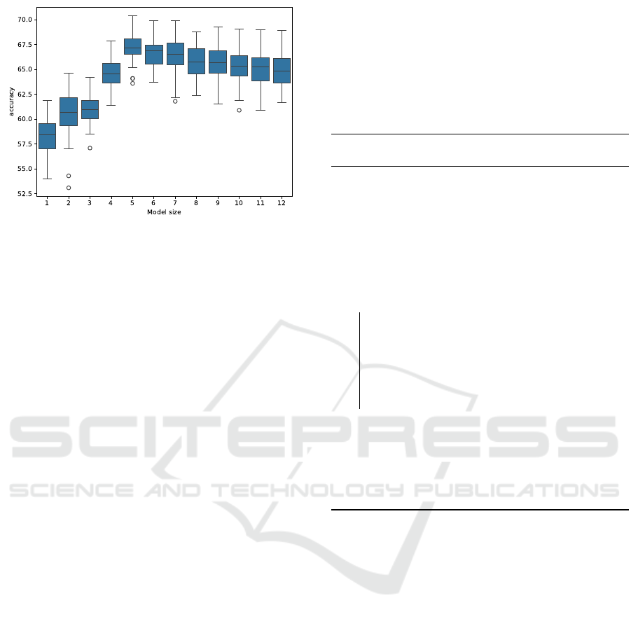
Figure 5: Accuracy on test data of models of different sizes

returned by GPASDiscrimination (originally published in

Nunkesser (2008)).

seems to be no way to distinguish between the un-

derlying interactions and similarly important interac-

tions. It is therefore desirable to extend GPAS with a

method to select the best model size automatically.

5 AUTOMATIC MODEL

SELECTION FOR GPAS

GPAS is available as an open source R package from

GitHub. However, a direct extension of GPAS on a

source code basis is not advisable as the sources have

heterogenous dependencies and the best model size

selection algorithm should be chosen ﬁrst to justify

the effort to change the code.

We therefore propose using GPAS as a black

box and applying an external method for automatic

model selection. For the black box algorithm, we can

use GPASDiscrimination and GPASInteractions

as described above.

5.1 GPASDiscrimination

The simulation results from Section 4.4 suggest that

GPASDiscrimination is capable of ﬁnding the true

model if the model size is automatically chosen

correctly. In a typical run on the simulated data,

GPASDiscrimination proposes models with sizes

between 1 and 12 literals.

Nunkesser (2008) gives more detailed insight into

the challenges in automatic model size selection for

GPAS. Figure 5 shows the accuracy on test data of

models of different sizes returned by GPASDiscrimi-

nation.

As mentioned before, Nunkesser (2008) describes

approaches for automatic model size selection in

GPAS which were not integrated into the available

algorithm. In this paper, we propose using a cross-

validation approach instead to automatically select

the best model size. Cross-validation is a standard

method to prevent overﬁtting not attempted in GPAS

before. We propose the approach described by Algo-

rithm 1 to automatically select the best model size.

Algorithm 1: Automatic Model Selection in

GPASDiscrimination.

Input: Data set, Cross-validation strategy,

Consolidation strategy, Selection

strategy

Output: Chosen polynomial

1 Use the cross-validation strategy to split the

data set into a set of training and validation

data pairs;

2 foreach Pair of training and validation data

3 Call GPASDiscrimination with the

training data set;

4 Compute the accuracies of the returned

models on the validation data set;

5 Add the returned models to a list of

candidate models;

6 end

7 Consolidate the list of candidate models with

the consolidation strategy;

8 Select a model from the candidate list with

the selection strategy;

9 return The chosen model

Initial experiments on the data from Section 4.4

suggest, that the following choices offer a very

promising automatic model selection: For cross vali-

dation, 5-fold cross validation is chosen. The consol-

idation strategy works as follows:

1. Discard all models that do not appear in all of the

5 runs on the folds.

2. Discard all models where a model of the same size

with a better average accuracy on the validation

data exists.

Lastly, as a selection strategy, the accuracy gain with

regard to larger model sizes is considered. Large

models that do not at least offer 1% more accuracy

than all smaller models are discarded. Afterwards,

the model with the greatest accuracy is chosen.

In a simulation with the data used in Section 4.2,

the algorithm has chosen the real underlying model in

71 out of 100 runs. Figure 6 shows a summary.

The mean accuracy of the models chosen by

GPAS is 0.666 with a standard deviation of 0.019

(while the true model would result in an accuracy

Highly Interpretable Prediction Models for SNP Data

559

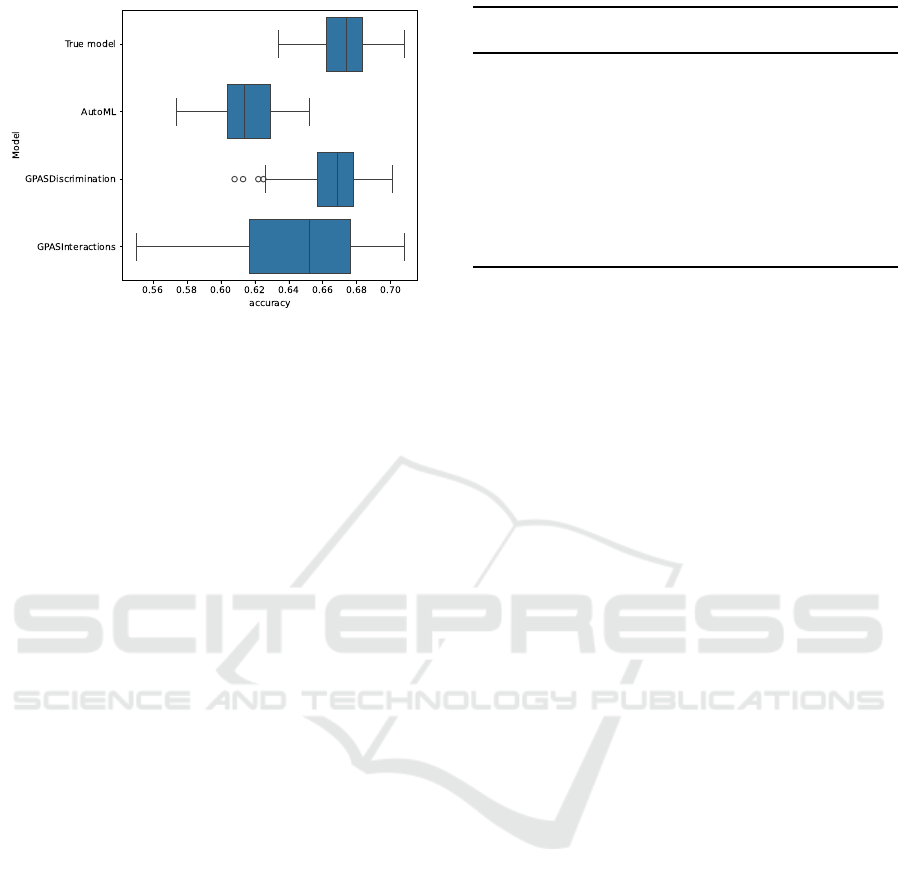
Figure 6: Accuracy on test data of the underlying model and

the model chosen by AutoML and GPAS.

of 0.673 with a standard deviation of 0.015). This

is comparable to the results achieved by Nunkesser

(2008). However, the method proposed here is more

general and easier to parameterize. The results are

promising, but the approach is not yet fully devel-

oped. Future research must show if the choice of dif-

ferent parameters may yield better results and how the

concept performs on further simulated data.

5.2 GPASInteractions

It is possible to extend Algorithm 1 to

GPASInteractions in a straightforward way.

Only the most frequent interactions are kept in

the interaction tree. This approach will not be

investigated further here, as it appears sensible to

investigate further and optimize the approach for

GPASDiscrimination ﬁrst.

Apart from cross-validation, in the case of

GPASInteractions, we can also use a pruning

method for the interaction tree. The simula-

tion results from Section 4.4 already suggest that

GPASInteractions is capable of ﬁnding the true

model if the pruning method for the interaction tree

is chosen correctly. We propose using Algorithm 2 to

automatically prune the interaction tree.

In an initial simulation with the data used in Sec-

tion 4.4 and t

= 0.2,t

= 0.75 the algorithm has cho-

sen the real underlying model in 56 out of 100 runs.

Figure 6 shows a summary of the runs. As men-

tioned above, GPASInteractions is intended as an

interesting alternative for real data, as it may show

more interactions than GPASDiscrimination. With-

out pruning, the results tend to be very large and less

interpretable. The pruning approach proposed here is

a ﬁrst step to making the method more interpretable

and preventing overﬁtting while still maintaining the

greater variety of results.

Algorithm 2: Automatic Tree Pruning in GPAS-

Interactions.

Input: Data set, Root frequency threshhold

, Subtree frequency threshold t

Output: Pruned interaction tree

1 Call GPASInteractions with the data set;

2 Prune all subtrees with a root frequency

below t

;

3 Prune all subtrees with a frequency of a

non-root-node below t

;

4 return The pruned interaction tree

6 FUTURE WORK

The approach proposed here is a ﬁrst step in extend-

ing GPAS with automatic model selection. Further

research is needed before integrating the selection

method into the existing algorithm.

6.1 Application to Further Data

Future research must show whether the choice of dif-

ferent parameters yields better results and how the

concept performs on further data. The parameteriza-

tion encompasses the choice of the cross-validation

strategy, the consolidation strategy, and the selection

strategy. In order to further substantiate these results,

further studies on different data are necessary. The

next obvious data sets are:

1. More sophisticated simulations based on scrime

such as the ones used in Lau et al. (2022).

2. More general dichotomized data such as that used

in Lau et al. (2024).

3. Ordinal data with the extension to GPAS proposed

in Nunkesser (2008)

After the results on these data sets are available,

the next steps should be the application of the ap-

proach to real data and the integration of the selection

method into the existing algorithm.

6.2 Generalization of the Method

The comparisons with the state-of-the-art algorithms

chosen by AutoML should be extended to the new

data sets. If it is conﬁrmed that an algorithm based

on Genetic Programming is capable of achieving or

even outperforming state-of-the-art results, the next

step should be the further extension of the method to

multi-valued responses or other categorical predictors

besides SNPs.

BIOINFORMATICS 2025 - 16th International Conference on Bioinformatics Models, Methods and Algorithms

560

This may be the most challenging part of the re-

search, as the methods are currently only designed for

binary responses and SNP data. At the moment two

alternatives seem sensible: generalizing the used dis-

junctive normal forms or extending the methods to de-

cision diagrams.

6.2.1 Generalizing Disjunctive Normal Forms

A possible extension of the used literals

• SNP

= AA

• SNP

̸= AA

• SNP

= Aa/aA

• SNP

̸= Aa/aA

• SNP

= aa

• SNP

̸= aa

to general nominal data is to use the generalizable lit-

erals

• SNP

∈ {AA}

• SNP

∈ {Aa/aA,aa}

• SNP

∈ {Aa/aA}

• SNP

∈ {AA,aa}

• SNP

∈ {aa}

• SNP

∈ {AA,Aa/aA}

instead. A challenge is of course to deal with the ex-

ponentially growing search space.

A possible extension for multi-valued responses

is to abandon boolean algebra and exchange it for a

more general algebra. If we replace ∧ by × and ∨ by

+ and introduce weight vectors, a model like

(SNP6 ̸= AA)(SNP7 = AA)

∨ (SNP3 = AA)(SNP9 = AA)(SNP10 = AA)

could be expressed as:









SNP6 ∈ {Aa/aA, aa}SNP7 ∈ {AA}





SNP3 ∈ {AA}SNP9 ∈ {AA}SNP10 ∈ {AA}

After an application of the softmax function, the

model could yield probabilities for different classes

and is generalizable to multi-valued responses.

6.2.2 Extending the Method to Decision

Diagrams

If the approach of using disjunctive normal forms

or a generalization of them as a model is no longer

sufﬁcient, an extension to decision diagrams is con-

ceivable. There are already investigations being con-

ducted here in the context of Genetic Programming

(see e.g. Droste, 1997; Wegener, 2000). In recent re-

sults, Florio et al. (2023) propose to use Decision Di-

agrams trained by MILP while Hu et al. (2022) use

MaxSAT. However, as Florio et al. (2023) state:

Most likely, the biggest obstacle towards the

effective use of decision diagrams remains the

ability to learn them efﬁciently.

It is an interesting question how an approach

based on Genetic Programming would perform in

comparison.

7 CONCLUSION

In this paper, we have shown that highly interpretable

prediction models for SNP data are important for

understanding possible underlying biological mech-

anisms. We have also shown that logicFS, GPAS, and

logicDT are capable of yielding highly interpretable

prediction models. The automatic prevention of over-

ﬁtting requires improvement, however. We have pro-

posed using GPAS as a black box and applying an ex-

ternal method for automatic model selection. We have

presented an approach using the GPAS algorithm as

a black box and shown initial results on simulated

data. The initial results are comparable to the results

achieved by Nunkesser (2008). The approach offers

an easier parameterization and is more general, how-

ever. Future research must demonstrate whether the

choice of different parameters yields better results and

how the concept performs on other simulated data. As

this paper presents work in progress, the outlook on

future work is of great interest.

REFERENCES

Bureau, A., Dupuis, J., Falls, K., Lunetta, K. L., Hayward,

B., Keith, T. P., and Van Eerdewegh, P. (2005). Iden-

tifying snps predictive of phenotype using random

forests. Genetic Epidemiology, 28(2):171–182.

Che, R. and Motsinger-Reif, A. (2013). Evaluation of ge-

netic risk score models in the presence of interaction

and linkage disequilibrium. Frontiers in Genetics, 4.

Chen, C. C., Schwender, H., Keith, J., Nunkesser, R.,

Mengersen, K., and Macrossan, P. (2011). Methods

for identifying snp interactions: A review on varia-

tions of logic regression, random forest and bayesian

logistic regression. IEEE/ACM Transactions on Com-

putational Biology and Bioinformatics, 8(6):1580–

1591.

Highly Interpretable Prediction Models for SNP Data

561

Droste, S. (1997). Efﬁcient genetic programming for ﬁnd-

ing good generalizing Boolean functions. In Koza,

J. R., Deb, K., Dorigo, M., Fogel, D. B., Garzo, M.,

Iba, H., and Riolo, R. L., editors, Proceedings of the

Second Annual Conference on Genetic Programming,

pages 82–87, San Francisco, Calif. Morgan Kaufmann

Publishers, Inc.

Florio, A., Martins, P., Schiffer, M., Serra, T., and Vidal,

T. (2023). Optimal decision diagrams for classiﬁ-

cation. In Williams, B., Chen, Y., and Neville, J.,

editors, AAAI-23 Technical Tracks 6, Proceedings of

the 37th AAAI Conference on Artiﬁcial Intelligence,

AAAI 2023, pages 7577–7585. AAAI Press.

Garte, S. (2001). Metabolic Susceptibility Genes As Cancer

Risk Factors: Time for a Reassessment? Cancer Epi-

demiology, Biomarkers & Prevention, 10(12):1233–

1237.

Hu, H., Huguet, M.-J., and Siala, M. (2022). Optimizing bi-

nary decision diagrams with maxsat for classiﬁcation.

Proceedings of the AAAI Conference on Artiﬁcial In-

telligence, 36:3767–3775.

International Human Genome Sequencing Consortium

(2001). Initial sequencing and analysis of the human

genome. Nature, 409(6822):860–921.

Lau, M., Schikowski, T., and Schwender, H. (2024). log-

icDT: a procedure for identifying response-associated

interactions between binary predictors. Machine

Learning, 113(2):933–992.

Lau, M., Wigmann, C., Kress, S., Schikowski, T., and

Schwender, H. (2022). Evaluation of tree-based sta-

tistical learning methods for constructing genetic risk

scores. BMC Bioinformatics, 23(1):97.

Nunkesser, R. (2008). Analysis of a genetic program-

ming algorithm for association studies. In GECCO

’08: Proceedings of the 10th Annual Conference on

Genetic and Evolutionary Computation, pages 1259–

1266, New York. ACM.

Nunkesser, R., Bernholt, T., Schwender, H., Ickstadt, K.,

and Wegener, I. (2007). Detecting high-order in-

teractions of single nucleotide polymorphisms using

genetic programming. Bioinformatics, 23(24):3280–

3288.

Ruczinski, I., Kooperberg, C., and L. LeBlanc, M. (2004).

Exploring interactions in high-dimensional genomic

data: an overview of logic regression, with applica-

tions. Journal of Multivariate Analysis, 90(1):178–

195.

Rudin, C., Chen, C., Chen, Z., Huang, H., Semenova, L.,

and Zhong, C. (2022). Interpretable machine learn-

ing: Fundamental principles and 10 grand challenges.

Statistics Surveys, 16:1 – 85.

Schwender, H. and Fritsch, A. (2018). scrime: Analysis

of High-Dimensional Categorical Data such as SNP

Data. R package version 1.3.5.

Schwender, H. and Ickstadt, K. (2007). Identiﬁcation of

SNP interactions using logic regression. Biostatistics,

9(1):187–198.

Tong, H., Küken, A., Razaghi-Moghadam, Z., and

Nikoloski, Z. (2021). Characterization of effects

of genetic variants via genome-scale metabolic mod-

elling. Cellular and Molecular Life Sciences,

78(12):5123–5138.

Wegener, I. (2000). Branching Programs and Binary Deci-

sion Diagrams. SIAM, Philadelphia.

Winham, S. J., Colby, C. L., Freimuth, R. R., Wang,

X., de Andrade, M., Huebner, M., and Biernacka,

J. M. (2012). SNP interaction detection with Random

Forests in high-dimensional genetic data. BMC Bioin-

formatics, 13(1):164.

BIOINFORMATICS 2025 - 16th International Conference on Bioinformatics Models, Methods and Algorithms

562