A Parallel Implementation of the Clarke-Wright Algorithm on GPUs

Francesca Guerriero

and Francesco Paolo Saccomanno

Department of Mechanical, Energy and Management Engineering,

University of Calabria, Ponte Pietro Bucci, 87036 Rende, Italy

{francesca.guerriero, francescopaolo.saccomanno}@unical.it

Keywords:

Capacitated Vehicle Routing Problem, CVRP, Clarke-Wright Algorithm, GPU Computing, CUDA, Heuristics.

Abstract:

The Clark & Wright (CW) algorithm is a greedy approach, aimed at ﬁnding good-quality solutions for the

capacitated vehicle routing problem (CVRP). It is the most widely applied heuristic algorithm to solve CVRP

due to its simple implementation and effectiveness. In this work, we propose a parallel implementation of the

CW algorithm well suited to be executed on GPUs. In order to evaluate the performance of the developed

approach, an extensive computational phase has been carried out, by considering a large set of test problems.

The results are very encouraging, showing a signiﬁcant reduction in computational time compared to the

sequential version, especially for large-scale networks.

1 INTRODUCTION

The Capacitated Vehicle Routing Problem (CVRP)

is a NP-Hard combinatorial optimization problem

(Laporte, 1992), which seeks to determine an opti-

mal set of routes for a ﬂeet of vehicles, with lim-

ited capacity to deliver goods to customers, while

minimizing the total transportation cost. Due to its

NP-hard nature, ﬁnding exact solutions for large-

scale instances is computationally intractable, there-

fore, optimal solutions can be found only when a

limited number of nodes (customers and depot) are

considered. For more complex scenarios, heuris-

tics and meta-heuristics have been developed to ﬁnd

approximate optimal solutions, (Accorsi and Vigo,

2021), (Liu et al., 2023). Among these, the Clarke-

Wright algorithm (CW) is a greedy approach widely

used for its efﬁciency and effectiveness in address-

ing the CVRP through a simple approach, (Clarke and

Wright, 1964), (Augerat et al., 1995). In particular, it

relies on building a list of possible savings, obtained

when two routes are merged, followed by iterative

merging of routes if the constraints of the problem

are satisﬁed. Despite its simplicity, the CW approach,

based on savings, can achieve results within 7% of

the optimal value, especially for large instances. In

the scientiﬁc literature, several authors have proposed

improvements to the CW algorithm to enhance its ef-

fectiveness or address other variants of the CVRP,

https://orcid.org/0000-0002-3887-1317

https://orcid.org/0000-0002-8807-8659

(Bor

cinov

a, 2022), (Nurcahyo et al., 2023), (Tun-

nisaki and Sutarman, 2023). Parallel computing sys-

tems also offer a viable approach for developing solu-

tion methods capable of solving large-scale CVRPs.

In this work, we propose a parallel implementation of

the basic CW algorithm on GPU.

In what follows, a concise overview of the lit-

erature related to the development of parallel ap-

proaches to solve the CVRP is provided. Attention

is focused on the scientiﬁc contributions most rele-

vant to our study. Previous studies have primarily

focused on parallelizing existing metaheuristics us-

ing GPUs to enhance execution speed. These works

used graphics processors to handle speciﬁc portions

of the code. For example, (Benaini and Berrajaa,

2018) proposed a GPU-accelerated evolutionary ge-

netic algorithm for dynamic vehicle routing prob-

lems (DVRP), in which requests can occur later. The

proposed approach is able to ﬁnd good-quality solu-

tions for up to 3,000 nodes. Similarly, (Abdelatti and

Sodhi, 2020) parallelized a genetic algorithm with lo-

cal search strategies. Other works used ant colony

optimization (Diego et al., 2012), which determines

the solution to the problem by imitating the behavior

of certain insects in nature, and local search methods

(Luong et al., 2013), which iteratively move from one

solution to another in a given neighborhood. Simi-

larly, the local search approach is used in (Schulz,

2013). In particular, the two classical heuristics 2-

opt and 3-opt were implemented in parallel on GPUs.

The instances considered include CVRP and DVRP

100

Guerriero, F. and Saccomanno, F. P.

A Parallel Implementation of the Clarke-Wright Algorithm on GPUs.

DOI: 10.5220/0013138100003893

Paper published under CC license (CC BY-NC-ND 4.0)

In Proceedings of the 14th International Conference on Operations Research and Enterprise Systems (ICORES 2025), pages 100-111

ISBN: 978-989-758-732-0; ISSN: 2184-4372

problems, ranging from 57 to 2400 nodes.

In (Jin et al., 2014), a tabu search approach is con-

sidered, in which the threads work in parallel for the

intensiﬁcation and diversiﬁcation phase. The authors

have achieved effective results in instances with up to

1,200 nodes.

In (Boschetti et al., 2017), the authors used

dynamic programming and a relaxation approach,

namely state-space relaxation, to compute the bounds.

Since these methods are time-consuming, they devel-

oped a GPU computing approach and proved that it

is capable of achieving up to 40 times time reduction

compared to the sequential version, when solving an

instance with 2,000 nodes.

(Benaini et al., 2016) presented a GPU-based

heuristic for single and multi-depot VRPs, generat-

ing initial solutions in parallel and progressively re-

ﬁning them. Unlike our approach, which directly op-

timizes the CW algorithm’s steps, their method uses

GPUs to generate multiple initial solutions and re-

lies on the standard CW algorithm. In subsequent

works, (Benaini and Berrajaa, 2016), (Benaini et al.,

2017) developed GPU implementations for dynamic

request insertion and multi-capacity VRPs, respec-

tively. More recent studies, such as (Yelmewad and

Talawar, 2021), have focused on improving the per-

formance of local search heuristics using GPUs.

To the best of our knowledge, the only CUDA-

based approach aimed at implementing the basic CW

algorithm on GPUs has been presented in (Guerriero

and Saccomanno, 2024). This early research ad-

dresses the merging of tasks sequentially and focuses

on cases with a relatively small number of nodes, pri-

marily due to memory constraints. The present paper

addresses these limitations and provides a more efﬁ-

cient parallel version of the CW algorithm.

Contribution and Organization of the Paper.

This work focuses on developing the CW heuristic

on GPUs to enhance performance. A comparison be-

tween the GPU implementation and its CPU coun-

terpart reveals signiﬁcant speed-ups achieved by the

GPU, especially for large-scale instances.

The main contributions of this paper are the fol-

lowing:

• development and testing of a parallel version of

CW steps, by exploiting GPU capability;

• design and implementation of CUDA Kernel ad-

hoc for the calculation of Distance/Cost Matrix

and relative savings;

• implementation of a benchmark system to analyse

each step of CW algorithm;

• deﬁnition of an approach for reducing in parallel

the number of operations to be executed sequen-

tially on the CPU.

The structure of the paper is as follows. Sec-

tion 2 provides a summary of the steps involved in

the CW method, illustrating the process on a toy ex-

ample. Section 3 outlines the proposed parallel ap-

proach. Section 4 focuses on the analysis of the com-

putational results, collected in an extensive experi-

mental phase. The paper concludes with ﬁnal obser-

vations in Section 5.

2 THE CW ALGORITHM

The CW approach can be viewed as divided into four

main phases: calculating the distance/cost matrix, cal-

culating the savings list, sorting, and ﬁnally merging

the routes. The cost calculation is typically based

on the Euclidean distance between nodes, but other

metrics can be used. Furthermore, distances are usu-

ally rounded to the nearest integer in experiments, as

ﬂoating-point calculations are much slower.

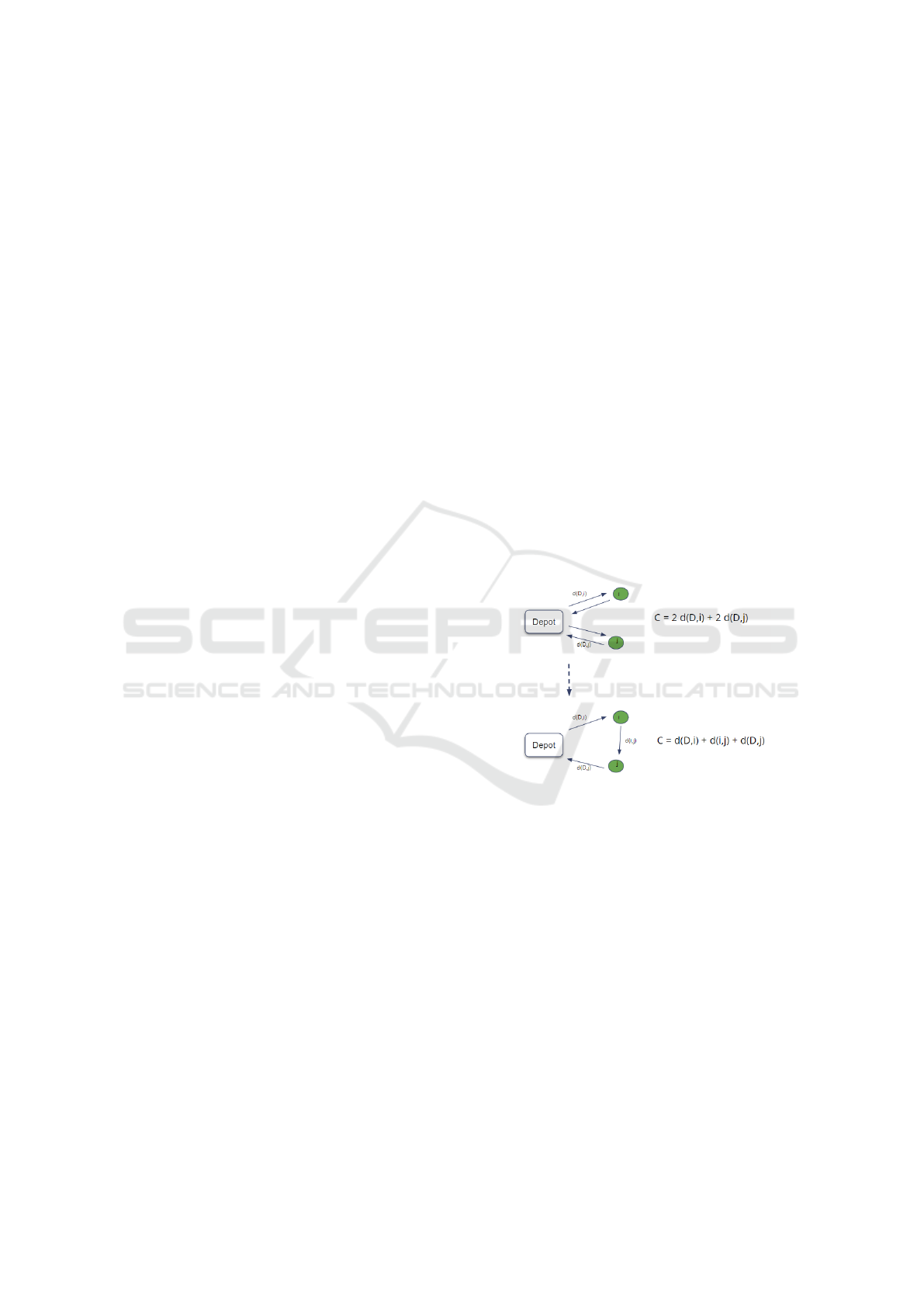
Figure 1: Saving with node i and j.

The list of savings is calculated as the cost reduc-

tions that can be achieved when a vehicle transports

goods to node i starting from another node j, instead

of starting again from the depot d (see Fig. 1):

Saving(i, j) = d(D, i) + d(D, j) − d(i, j). (1)

In practice, even though it adds a trip and there-

fore a cost between the nodes i and j , it allows the

elimination of two other trips: one between the depot

and the nodes i and another between the depot and the

node j. Subsequently, before starting route merging,

this list of savings is reordered according to decreas-

ing values, allowing the largest savings values to be

considered ﬁrst.

There are two versions of route merging: sequen-

tial and parallel. However, these terms do not refer

A Parallel Implementation of the Clarke-Wright Algorithm on GPUs

101

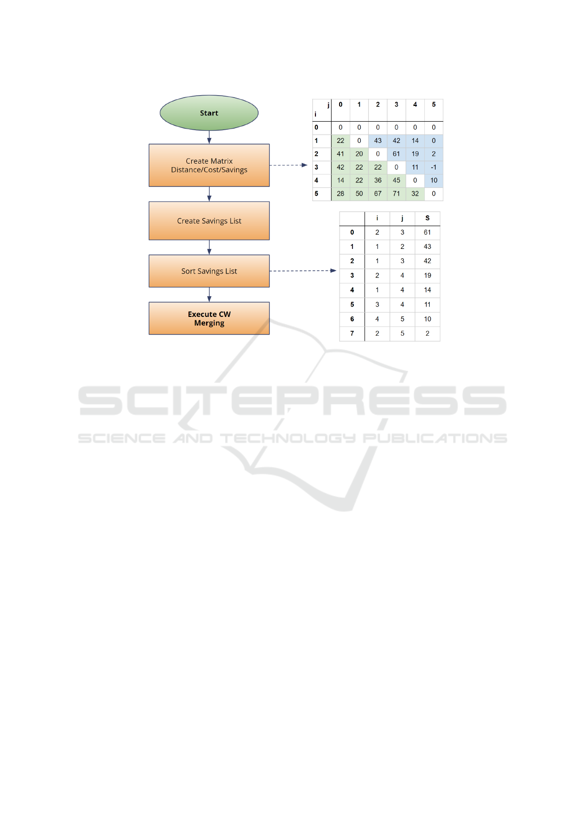
Figure 2: Schematization of the CW algorithm.

to execution on speciﬁc hardware, but rather they de-

scribe how the elements of the savings list are pro-

cessed. In the former, the sequential, one route at

a time, is completed by sequentially considering the

items in the savings list and inserting the nodes that

do not violate the constraints. The next route is con-

sidered when it is no longer possible to insert further

savings into the current one. In the parallel case, in-

stead, an element of the saving list is extracted in se-

quence and the two indicated routes are merged, al-

ways taking into account the constraints. In this case,

therefore, during iterations, multiple routes are con-

sidered “in parallel”.

The performance of the sequential approach

presents an average gain compared to the optimal so-

lution of 18%, while in the parallel case, it improves

to 7% (Caccetta et al., 2013). For this reason, we will

use only the parallel variant of CW in both the CPU

and GPU implementations.

In detail, in the parallel case, the merging steps are

as follows:

1. The next element of the savings list sorted in de-

scending order is extracted.

2. The constraints are veriﬁed: in this work, only the

vehicle capacity restrictions are considered, even

though it is possible to easily modify the approach

to consider time windows or incompatibilities be-

tween goods constraints.

3. If the constraints are satisﬁed, if neither of the two

nodes i, j is assigned, a new route is created.

4. Otherwise, the unassigned node is added to the

route or the two routes are merged.

To explain how the CW algorithm works, it is use-

ful to consider a toy example made up of six nodes

with the following coordinates in the Euclidean space:

[10, 20], [10, 40], [30, 30], [-10, 10], [-20, -20] and

the depot on [0,0]. The costs, i.e., the distances, are

then calculated based on these coordinates (as de-

picted in Fig. 2). Suppose that the corresponding de-

mand vector is [50, 50, 50, 25, 25] and the vehicle

capacity is 100. The ﬁrst operations to be performed

involve calculating the Cost Matrix and the creation

and ordering of the Savings List (Fig. 2). Then each

link in the savings list is considered: the ﬁrst one

(2,3), since both nodes are unassigned, involves creat-

ing a new tour {2,3} with a load 50 +50 = 100, equal

to the maximum capacity of the vehicles. After, the

links (1,2) and (1,3) are discarded, since nodes 2 and

3 are already present in the tour {0,2,3,0}, but the ve-

hicle is already full. The iteration proceeds with dis-

carding (2,4), and with the creation of a new tour for

the link (1,4) (i.e., {0,1,4,0}), which reaches a load of

75. Then the link (3,4) is discarded, since the nodes

3 and 4 are already assigned to two different routes.

Finally, the link (4,5) is added to obtain from the sec-

ond tour the new tour {0, 1, 4, 5, 0}. Obviously, the

remaining links (2,5) and (3,5) will be discarded. Af-

ter processing all the elements of the savings list, the

ICORES 2025 - 14th International Conference on Operations Research and Enterprise Systems

102

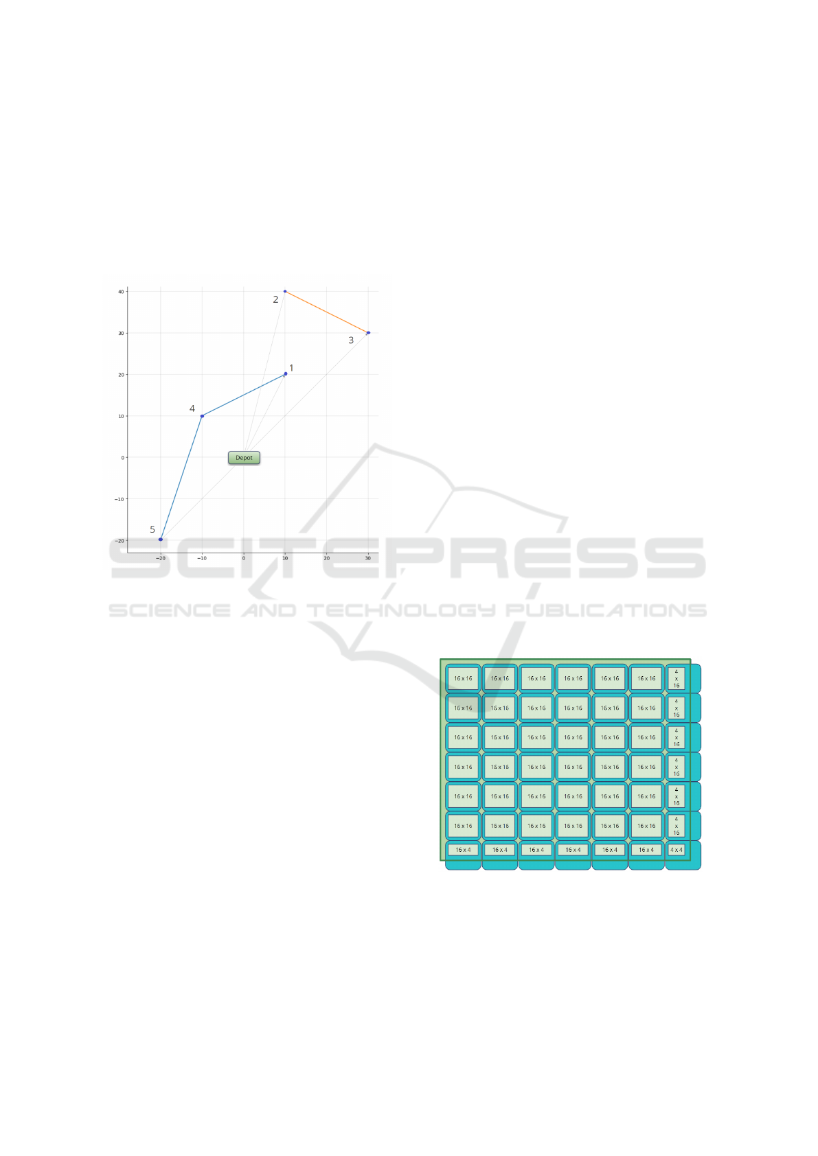
obtained solution (Fig. 3) will consist of only two

routes: {0,2,3,0},{0,1,4,5,0}. It is worth noting

that, after processing saving (4,5), node 4 becomes

internal to the route, allowing us to ignore any sub-

sequent links in the list, where node 4 appears. This

key idea will be used in our approach to reduce the

remaining items belonging to the savings list, and, in

our approach, this reduction will be performed con-

currently on GPU.

Figure 3: Example with six nodes.

The description provided highlights that although

the elements of the savings list require sequential pro-

cessing, both the computation of the distance/cost ma-

trix and the generation of the savings list can be opti-

mized using parallelization. Consequently, this study

aims to implement these steps in parallel by exploiting

GPU capabilities and analyzing the potential speed-

up over traditional CPU-based processing. As illus-

trated in the toy example, an alternative technique for

the merging phase will also be developed to effec-

tively use the GPU: the list is handled sequentially,

but reduced through a parallel method. In the sub-

sequent section, the details of this approach will be

clariﬁed.

3 THE CW ALGORITHM ON GPU

(CWG)

The purpose of this work is to improve the ef-

ﬁciency of the basic CW approach, by using a

GPU. GPUs were created to improve graphics perfor-

mance, but were later used for mathematical model-

ing and solving optimization problems. Unlike CPUs,

which have a few highly performant cores, GPUs are

equipped with thousands of cores capable of perform-

ing simpler computations. Among the various usage

paradigms, NVidia, one of the GPU brands, intro-

duced the CUDA framework, which allows for ab-

straction from the physical structure of the graphics

card: the functions to be executed in the threads are

called kernels, identical for all threads but operating

on different data. The various threads are logically

grouped into blocks and the blocks are grouped into a

grid. The size of the blocks depends on the problem

at hand and the resources needed. Each thread uses

a private local memory and a shared memory with all

other threads in the same block. These memories are

fast, but limited, and restrict the maximum number of

threads that can be executed in a block. There is also

a global memory, which is accessible to all threads in

the grid, slower than the previous ones, but generally

with capacities reaching up to tens of gigabytes.

CUDA requires the division of processing capac-

ity into blocks made up of t x t threads. A common

choice is to use blocks of 32 x 32 or 16 x 16 threads, as

these conﬁgurations provide a good balance between

computational efﬁciency and compatibility across dif-

ferent GPU architectures. Currently, the maximum

number of threads per block in CUDA is 32 x 32 =

1,024. While using a high number of threads might

seem advantageous, it can often result in some threads

remaining unused. The optimal number of threads per

block depends on several factors: the actual number

of threads needed for the computation, the available

local memory resources per block, and the perfor-

mance achieved with different block sizes.

Figure 4: Covering a 100 x 100 matrix using 7 x 7 blocks

of 16 x 16 threads.

To better explain the ﬁrst point, that is, the need

to determine the right number of threads to be used,

it is useful to consider the example of a matrix with

100 nodes (see Fig. 4), for which the number of op-

A Parallel Implementation of the Clarke-Wright Algorithm on GPUs

103

erations to be executed (i.e. the cells of the matrix) is

100 x 100 = 10,000. If a block of 16 x 16 threads is

chosen, a minimum number of 7 x 7 blocks is needed,

for a total of 12,544 threads, therefore the 20.28% of

threads remain unused. As illustrated in the ﬁgure,

the ﬁnal blocks of threads are only partially utilized,

leading to some threads being left idle.

Table 1: Unused threads for different thread block conﬁgu-

ration.

Nodes Num. Block Size Min Block Numbers Unused

100 32 x 32 4 x 4 38.96%

300 32 x 32 10 x 10 12.11%

500 32 x 32 16 x 16 4.63%

1000 32 x 32 32 x 32 4.63%

3000 32 x 32 94 x 94 0.53%

5000 32 x 32 157 x 157 0.95%

6000 32 x 32 188 x 188 0.53%

10000 32 x 32 313 x 313 0.32%

20000 32 x 32 626 x 626 0.32%

50000 32 x 32 1563 x 1563 0.06%

100 16 x 16 7 x 7 20.28%

300 16 x 16 19 x 19 2.61%

500 16 x 16 32 x 32 4.63%

1000 16 x 16 63 x 63 1.58%

3000 16 x 16 188 x 188 0.53%

5000 16 x 16 313 x 313 0.32%

6000 16 x 16 376 x 376 0.53%

10000 16 x 16 626 x 626 0.32%

20000 16 x 16 1251 x 1251 0.16%

50000 16 x 16 3126 x 3126 0.06%

100 8 x 8 13 x 13 7.54%

300 8 x 8 38 x 38 2.61%

500 8 x 8 63 x 63 1.58%

1000 8 x 8 126 x 126 1.58%

3000 8 x 8 376 x 376 0.53%

5000 8 x 8 626 x 626 0.32%

6000 8 x 8 751 x 751 0.27%

10000 8 x 8 1251 x 1251 0.16%

20000 8 x 8 2501 x 2501 0.08%

50000 8 x 8 6251 x 6251 0.03%

Tab. 1 shows the amount of unused threads as a

function of the number of nodes N and block size.

The column “Min Block Numbers” represents the

minimum block size of threads to cover the matrix.

The last column indicates the percentage of unused

threads: this drops below 5% in the case of problems

with more than 500 nodes, which are the problems

considered in this paper.

The CW algorithm was proﬁled to identify which

speciﬁc steps to be implemented in parallel, by us-

ing CUDA. Furthermore, this initial analysis allowed

us to optimize the various steps of the CPU ap-

proach, avoiding the various bottlenecks, including

those related to the use of the speciﬁc programming

language used in the computational phase (that is,

Python). This empowers the CPU version efﬁciently

even on medium/large instances, and additionally en-

ables a more effective evaluation of the performance

improvement using GPU. As expected, most of the

time is spent calculating the distance/cost matrix, cre-

ating the savings list, and merging processing in the

main loop. For this reason, we have built an ad-

hoc CUDA kernel that allows the ﬁrst two phases of

the algorithm to be completed in parallel. Instead,

for the sorting phase we relied on the cupy library

(https://cupy.dev/) which already offers efﬁcient sort-

ing algorithms based on CUDA. For the last merging

phase, we provided a reduction approach that aims to

ﬁlter the number of savings to analyze, the procedure

of which will be described in the next paragraph.

Fig. 5 illustrates the distance/cost matrix to be

computed. Each element below the diagonal repre-

sents the distance between the nodes, while the ele-

ments above the diagonal indicate the possible sav-

ings obtained by joining the two nodes i and j. The

calculation performed by a thread in a given cell is

represented in the ﬁgure and reﬂects the explanations

presented in the previous section. From this matrix,

the elements above the diagonal are extracted in order

to form the savings list (see the lower part of the same

ﬁgure).

The matrix is computed using a CUDA kernel,

which takes care of calculating each of the elements in

parallel, therefore, if the number of nodes is N, NxN

threads are launched in parallel to compute this ma-

trix: half of these threads are responsible for comput-

ing the distances/costs (below the diagonal), and the

other half the savings between two nodes.

In practice, in parallel, each created thread takes

care of calculating a given element of the matrix using

formulas (2) and (1).

C =

− x

)

+ (y

− y

)

(2)

Then, the savings list is extracted in the same

CUDA kernel which, in a simple way, retrieves the

elements above the diagonal and copies them into a

contiguous array of savings. The number of threads

is equal to the number of possible links between the

nodes. Therefore, excluding the links to the depot, it

is given by:

Link

i, j

= N ∗ (N − 1)/2. (3)

Look Ahead Parallel Reduction (LAPR). In the

last stage, the iterations of the CW algorithm cannot

be executed in parallel, because the analysis of subse-

quent savings requires waiting for the previous ones

to be processed. A different approach has been devel-

oped to utilize the GPU: once a node x is inserted into

ICORES 2025 - 14th International Conference on Operations Research and Enterprise Systems

104

Figure 5: Representation of operations performed in the CUDA kernel.

a route r, if the node becomes internal to the same

route r, or if the route r has reached the maximum

capacity C of the vehicle, the node x cannot be con-

sidered any more; therefore, we can create a tabu list

which contains all nodes that cannot longer be con-

sidered. The key idea is to process in parallel the re-

maining elements of the savings list, on the basis of

a “looking ahead” strategy, and to remove all of them

that contain nodes belonging to the tabu list, i.e. node

that cannot be further inserted or merged in a route.

The performance improvements are particularly sig-

niﬁcant in the case of large-scale instances. In Sec-

tion 4, the beneﬁts related to the application of this

technique, in terms of reduction of the length of the

saving list at each iteration, will be highlighted.

Since the merging phase is executed on the CPU,

every time the reduction approach is executed on the

GPU, a certain overhead is experienced. This lim-

its the possibility of calling the procedure after each

node, as the overhead time would exceed the bene-

ﬁt of list reduction. To address this issue, the nodes

are inserted into a tabu list and only when a certain

number is reached, the parallel reduction procedure is

activated. This hyperparameter has been empirically

determined, as shown in Section 4.

4 COMPUTATIONAL RESULTS

In order to assess the performance of the proposed ap-

proach, computational experiments have been carried

out considering X instances from (Uchoa et al., 2017)

and the Belgium sets (Arnold et al., 2019). The choice

was made because the ﬁrst ones are the ones currently

most used in evaluating the performance of solution

approaches for the CVRP and because they include

easy-to-solve instances (starting from 100 nodes, but

we have selected those starting from 500), for assess-

ing the overhead of the parallel algorithm, as well as

more complicated cases (up to 1,000 nodes). The sec-

ond dataset (i.e., Belgium dataset) contains test net-

works with a number of nodes ranging from 3,000 to

30,000. However, due to memory constraints to in-

stantiate matrices and lists, we were able to consider

instances of up to 16,000 nodes on CPU. The compu-

tational experiments have been carried out by imple-

menting and comparing the following algorithms:

• CWG: the GPU-based parallel implementation of

the CW algorithm;

• CWG

: the ﬁrst version of CWG introduced in

(Guerriero and Saccomanno, 2024). This method

is similar to CWG. However, the primary differ-

ence lies in its approach of analyzing all items in

the savings list, due to the absence of the LAPR

procedure;

• CWC: the CPU-based implementation of the CW

algorithm;

• PyVRP: the state-of-art algorithm proposed in

(Wouda et al., 2024), based on an hybrid ge-

netic search algorithm that combines the global

search capabilities of genetic algorithms with lo-

cal search methods.

The code was developed in Python for both the

CPU and the GPU versions, whereas the CUDA ker-

nels were implemented using the NUMBA library.

The development environment used is COLAB, an

online platform offered by Google for the rapid devel-

opment of Python-based software. The environment

A Parallel Implementation of the Clarke-Wright Algorithm on GPUs

105

was linked to a local computing system to take advan-

tage of the PC in use equipped of an Intel i9-14900HX

2.2Ghz processor with 24 cores and 64GB of Ram,

and a RTX4090 laptop GPU with 16Gb GDDR5 fea-

turing 9728 CUDA cores.

In the subsequent sections, we will investigate

the inﬂuence of the dimensions of the thread blocks

on the performance, the solution quality achieved

through the CW method versus the best known so-

lution (BKS), the time comparison against the CWC

version, and how the LAPR method affects the num-

ber of savings. In addition, a comparison with the

state-of-art approach proposed in (Guerriero and Sac-

comanno, 2024) is also presented.

Impact of Thread Block Size on Performance.

The analysis performed in the previous section

showed that all threads per block conﬁgurations can

effectively exploit the number of active threads (see

Tab. 1), for the considered instances above 500 nodes,

as less than 5% of threads remain inactive.

In the Tab. 2, we report the execution times re-

quired by the initial two phases of the CWG algo-

rithm for instances belonging to the Belgium set, with

a number of nodes ranging from 3001 to 30001. The

columns indicate in order: the instance name, num-

ber of nodes, number of threads in a block (TxB),

and time of execution as min time (T

min

), max time

max

) and average time (T

avg

). The computational

results are averaged over 10 runs. This allowed us to

determine the minimum, maximum, and average exe-

cution times using thread blocks of sizes 8x8, 16x16,

and 32x32: although the average value does not differ

much, there is a slight advantage for the 16x16 block

conﬁguration.

The one with 16x16 threads per block is chosen as

it has proved to be the most effective.

Solution Quality Evaluation. In order to evalu-

ate the quality of the solutions determined by the

CWG approach, we compared the obtained results

with the BKS and with those found by the state-of-

the-art PyVRP algorithm, for which a time-limit of

60 seconds has been imposed for instances up to 1001

nodes, and 600 seconds for other instances. In partic-

ular, for each test problem, the solution quality gap is

evaluated as

alg2

alg1

% =

alg1

− c

alg2

)

alg2

× 100,

where c represents the cost, and alg1 and alg2 re-

fer to the approaches under comparison (i.e., CWG,

PyVRP, or the BKS).

Table 2: Executions time for different number of threads per

block.

Instance Nodes TxB T

min

max

avg

Leuven1 3001 (8, 8) 0.03 0.12 0.0450

Leuven2 4001 (8, 8) 0.05 0.14 0.0710

Antwerp1 6001 (8, 8) 0.10 0.23 0.1559

Ghent1 10001 (8, 8) 0.33 0.48 0.3990

Ghent2 11001 (8, 8) 0.40 0.56 0.4730

Brussels1 15001 (8, 8) 0.76 0.99 0.9010

Brussels2 16001 (8, 8) 0.92 1.12 1.0290

Flanders1 20001 (8, 8) 1.34 1.56 1.4113

Flanders2 30001 (8, 8) 3.09 3.51 3.2363

Avg 0.8579

Leuven1 3001 (16, 16) 0.03 0.1 0.0426

Leuven2 4001 (16, 16) 0.05 0.13 0.0705

Antwerp1 6001 (16, 16) 0.10 0.22 0.1499

Ghent1 10001 (16, 16) 0.34 0.48 0.3990

Ghent2 11001 (16, 16) 0.39 0.62 0.4870

Brussels1 15001 (16, 16) 0.77 1.01 0.8600

Brussels2 16001 (16, 16) 0.83 1.09 0.9770

Flanders1 20001 (16, 16) 1.35 1.77 1.4763

Flanders2 30001 (16, 16) 3.00 3.18 3.1188

Avg 0.8423

Leuven1 3001 (32, 32) 0.03 0.11 0.0466

Leuven2 4001 (32, 32) 0.05 0.13 0.0718

Antwerp1 6001 (32, 32) 0.13 0.25 0.1610

Ghent1 10001 (32, 32) 0.36 0.53 0.4360

Ghent2 11001 (32, 32) 0.45 0.58 0.4980

Brussels1 15001 (32, 32) 0.81 0.97 0.8910

Brussels2 16001 (32, 32) 0.91 1.25 1.0310

Flanders1 20001 (32, 32) 1.38 1.66 1.4350

Flanders2 30001 (32, 32) 3.14 3.31 3.2125

Avg 0.8648

Tab. 3 gives the results for each instance. The ﬁrst

column lists the name of the test problem, followed

by the number of nodes in the second column, and the

BKS in the third column. The next two columns are

related to the PyVRP approach, displaying the solu-

tion cost c

PyV RP

and the solution quality gap δ

BKS

PyV RP

with the respect to the BKS. The ﬁnal columns sum-

marize the results for the CWG approach, including

the cost c

CWG

, the execution time t

CWG

and the so-

lution quality gap δ

BKS

CWG

% with respect to BKS and

PyV RP

CWG

% with respect to PyVRP.

For the small-size instances, CWG shows an aver-

age GAP of δ

BKS

CWG

% = 5.12% when compared to BKS,

and δ

PyV RP

CWG

% = 2.51% in comparison to PyVRP. For

larger instances from the Belgium Dataset, CWG in-

creases its performance, with δ

PyV RP

CWG

% being 1.60%,

0.53%, and 0.22% for different groups. CWG, on

the other hand, has signiﬁcantly reduced execution

times, requiring a maximum of t

CWG

= 183 seconds

for the largest scenario considered, which includes

ICORES 2025 - 14th International Conference on Operations Research and Enterprise Systems

106

Table 3: Benchmarking Solution Quality.

Instance Name Nodes BKS PyVRP CWG

PyVRP

BKS

% c

CWG

BKS

CWG

% δ

CWG

X-n502-k39 502 69226 69740 0.74% 71388 0.53 3.12% 2.36%

X-n513-k21 513 24201 24562 1.49% 26805 0.41 10.76% 9.13%

X-n524-k153 524 154593 155531 0.61% 163352 0.42 5.67% 5.03%

X-n536-k96 536 94846 96514 1.76% 99872 0.46 5.30% 3.48%

X-n548-k50 548 86700 88390 1.95% 89574 0.45 3.31% 1.34%

X-n561-k42 561 42717 43721 2.35% 45557 0.45 6.65% 4.20%

X-n573-k30 573 50673 51780 2.18% 52565 0.46 3.73% 1.52%

X-n586-k159 586 190316 193405 1.62% 199817 0.54 4.99% 3.32%

X-n599-k92 599 108451 111045 2.39% 113296 0.53 4.47% 2.03%

X-n613-k62 613 59535 60837 2.19% 62829 0.49 5.53% 3.27%

X-n627-k43 627 62164 63523 2.19% 65218 0.52 4.91% 2.67%

X-n641-k35 641 63682 66233 4.01% 67550 0.64 6.07% 1.99%

X-n655-k131 655 106780 107480 0.66% 108353 0.61 1.47% 0.81%

X-n670-k130 670 146332 148413 1.42% 158154 0.63 8.08% 6.56%

X-n685-k75 685 68205 69940 2.54% 71685 0.64 5.10% 2.49%

X-n701-k44 701 81923 84959 3.71% 85589 0.61 4.47% 0.74%

X-n716-k35 716 43373 45238 4.30% 45744 0.53 5.47% 1.12%

X-n733-k159 733 136187 140627 3.26% 139997 0.81 2.80% -0.45%

X-n749-k98 749 77269 79838 3.32% 79462 0.69 2.84% -0.47%

X-n766-k71 766 114417 117711 2.88% 119262 0.77 4.23% 1.32%

X-n783-k48 783 72386 75598 4.44% 76566 0.91 5.77% 1.28%

X-n801-k40 801 73305 76321 4.11% 76700 0.86 4.63% 0.50%

X-n819-k171 819 158121 161054 1.85% 166287 0.9 5.16% 3.25%

X-n837-k142 837 193737 198166 2.29% 200443 1.03 3.46% 1.15%

X-n856-k95 856 88965 90453 1.67% 92368 1.05 3.83% 2.12%

X-n876-k59 876 99299 102140 2.86% 102306 0.98 3.03% 0.16%

X-n895-k37 895 53860 56052 4.07% 58614 1.04 8.83% 4.57%

X-n916-k207 916 329179 334298 1.56% 343501 0.97 4.35% 2.75%

X-n936-k151 936 132715 137082 3.29% 146523 1.23 10.40% 6.89%

X-n957-k87 957 85465 87608 2.51% 89212 1.09 4.38% 1.83%

X-n979-k58 979 118976 121788 2.36% 123690 1.27 3.96% 1.56%

X-n1001-k43 1001 72355 75955 4.98% 77377 1.52 6.94% 1.87%

2.55% 5.12% 2.51%

Leuven1 3001 192848 200297 3.86% 200790 3.75 4.12% 0.25%

Leuven2 4001 111391 118483 6.37% 124194 3.49 11.49% 4.82%

Antwerp1 6001 477277 497588 4.26% 497009 4.83 4.13% -0.12%

Antwerp2 7001 291350 312371 7.22% 316878 7.57 8.76% 1.44%

5.43% 7.13% 1.60%

Ghent1 10001 469,531 491610 4.70% 488056 14.18 3.95% -0.72%

Ghent2 11001 257,748 277372 7.61% 283202 15.87 9.88% 2.10%

Brussels1 15001 501,719 533768 6.39% 529846 35.69 5.61% -0.73%

Brussels2 16001 345,468 373996 8.26% 379516 29.95 9.86% 1.48%

6.74% 7.32% 0.53%

Flanders1 20001 7240118 7542347 4.17% 7497837 54.74 3.56% -0.59%

Flanders2 30001 4373244 4716145 7.84% 4764789 182.57 8.95% 1.03%

6.01% 6.26% 0.22%

30K nodes.

The results indicate that the proposed CWG ap-

proach is capable of producing solutions of a quality

comparable to PyVRP, while offering substantial im-

provements in terms of computational time.

Time Analysis Against CWC Version. Table 4

presents the results obtained with CWC. In particu-

lar, the ﬁrst column displays the name of the instance,

whereas the second gives the number of nodes. The

subsequent columns display the total execution time

of the CWC approach (T

CWC

), the time spent creat-

A Parallel Implementation of the Clarke-Wright Algorithm on GPUs

107

Table 4: Time Analysis against CWC version.

Instance Nodes T

CWC

CWG

Speed-UP

X-n502-k39 502 1.40 0.77 0.45 0.01 0.17 0.53 0.01 0.00 0.01 0.51 3

X-n513-k21 513 1.58 0.98 0.35 0.01 0.24 0.41 0.01 0.00 0.00 0.40 4

X-n524-k153 524 1.37 0.68 0.41 0.02 0.26 0.42 0.01 0.00 0.00 0.41 3

X-n536-k96 536 1.23 0.69 0.35 0.01 0.18 0.46 0.01 0.00 0.00 0.45 3

X-n548-k50 548 1.36 0.75 0.41 0.01 0.19 0.45 0.01 0.00 0.00 0.44 3

X-n561-k42 561 1.65 0.97 0.46 0.01 0.21 0.45 0.01 0.00 0.00 0.44 4

X-n573-k30 573 1.59 0.84 0.48 0.01 0.26 0.46 0.01 0.00 0.00 0.45 3

X-n586-k159 586 1.61 0.94 0.40 0.01 0.26 0.54 0.01 0.00 0.00 0.53 3

X-n599-k92 599 1.66 0.90 0.47 0.01 0.28 0.53 0.01 0.00 0.00 0.52 3

X-n613-k62 613 1.66 1.00 0.42 0.01 0.23 0.49 0.01 0.00 0.00 0.48 3

X-n627-k43 627 1.77 1.02 0.49 0.01 0.25 0.52 0.01 0.00 0.00 0.51 3

X-n641-k35 641 1.92 1.14 0.52 0.01 0.25 0.64 0.01 0.00 0.00 0.63 3

X-n655-k131 655 2.06 1.15 0.55 0.02 0.34 0.61 0.01 0.00 0.01 0.59 3

X-n670-k130 670 1.91 1.08 0.51 0.01 0.31 0.63 0.01 0.00 0.01 0.61 3

X-n685-k75 685 2.23 1.22 0.60 0.04 0.37 0.64 0.01 0.00 0.01 0.62 3

X-n701-k44 701 2.35 1.42 0.62 0.02 0.29 0.61 0.01 0.00 0.01 0.59 4

X-n716-k35 716 2.77 1.51 0.77 0.04 0.45 0.53 0.01 0.00 0.01 0.51 5

X-n733-k159 733 2.51 1.42 0.68 0.02 0.39 0.81 0.01 0.00 0.01 0.79 3

X-n749-k98 749 2.44 1.44 0.66 0.01 0.33 0.69 0.01 0.00 0.01 0.67 4

X-n766-k71 766 2.45 1.48 0.62 0.02 0.33 0.77 0.01 0.00 0.01 0.75 3

X-n783-k48 783 2.64 1.53 0.71 0.02 0.38 0.91 0.01 0.00 0.01 0.89 3

X-n801-k40 801 2.84 1.55 0.81 0.03 0.45 0.86 0.01 0.00 0.01 0.84 3

X-n819-k171 819 2.88 1.60 0.83 0.02 0.43 0.90 0.01 0.00 0.01 0.88 3

X-n837-k142 837 3.01 1.74 0.79 0.02 0.46 1.03 0.01 0.00 0.01 1.01 3

X-n856-k95 856 3.14 1.74 0.87 0.03 0.50 1.05 0.02 0.00 0.01 1.02 3

X-n876-k59 876 3.53 1.99 0.99 0.03 0.52 0.98 0.01 0.00 0.01 0.96 4

X-n895-k37 895 3.32 1.87 0.92 0.03 0.50 1.04 0.01 0.00 0.01 1.02 3

X-n916-k207 916 3.83 2.14 1.05 0.03 0.61 0.97 0.01 0.00 0.01 0.95 4

X-n936-k151 936 4.17 2.29 1.15 0.03 0.70 1.23 0.01 0.00 0.01 1.21 3

X-n957-k87 957 4.09 2.28 1.17 0.06 0.58 1.09 0.01 0.00 0.01 1.07 4

X-n979-k58 979 4.15 2.42 0.97 0.04 0.72 1.27 0.01 0.00 0.01 1.25 3

X-n1001-k43 1001 4.47 2.62 1.20 0.03 0.62 1.52 0.02 0.00 0.01 1.49 3

Leuven1 3001 47.15 27.00 13.01 0.64 6.50 3.75 0.12 0.00 0.07 3.56 13

Leuven2 4001 84.70 46.48 24.33 1.29 12.60 3.49 0.21 0.00 0.03 3.25 24

Antwerp1 6001 186.33 114.14 46.20 2.87 23.12 4.83 0.34 0.00 0.08 4.41 39

Antwerp2 7001 207.33 120.09 53.91 3.98 29.35 7.57 1.09 0.00 0.12 6.36 27

Ghent1 10001 543.66 305.96 137.03 10.63 90.04 14.18 0.57 0.00 0.20 13.41 38

Ghent2 11001 657.45 370.74 181.01 11.95 93.75 15.87 0.74 0.00 0.57 14.56 41

Brussels1 15001 1073.02 570.40 275.92 25.19 201.51 35.69 1.06 0.00 0.61 34.02 30

Brussels2 16001 1393.93 777.41 373.63 30.97 211.92 29.95 1.11 0.00 0.55 28.29 47

Average 106.83 3.48 9.10

ing the distance/cost matrix (T

CWC

), generating the

savings list (T

CWC

), ordering (T

CWC

), and executing

merge iterations (T

CWC

). Similarly, times for CWG

operations on GPU are given (i.e., T

CWG

, T

CWG

, T

CWG

, T

CWG

). The last column displays the speed-up

achieved by the CWG compared to the CWC, calcu-

lated as

CWC

CWG

The results show the ability of the CWG approach

to scale in the calculation of the cost matrix and

the savings list. In particular, the higher the num-

ber of nodes, the higher the speed-up achieved. For

example, for the Brussels2 instance it reduces from

1151.04 seconds (i.e., 777.41 + 373.63 seconds) to

1.11 seconds.

It should be noted that in the case of the CWG

approach, the savings list creation time is equal to 0

since this, as we saw in the previous section, is calcu-

lated in parallel together with the cost matrix. As ex-

pected, the ﬁrst three phases, being entirely processed

on the GPU, beneﬁt from the maximum speed-up. Al-

though the ﬁnal route merging phase is performed on

the CPU, it still achieves signiﬁcant time improve-

ment due to the reductions provided by the LAPR pro-

cedure. For instance, in the Brussels2 case, the total

time decreases from 211.92 to 28.29 seconds.

Clearly, the performance improvements of the

CWG implementation compared to the CWC version

ICORES 2025 - 14th International Conference on Operations Research and Enterprise Systems

108

become more signiﬁcant for the latest set of test prob-

lems under consideration. In effect, the real potential

of the CWG becomes more evident in these latter in-

stances, characterized by a high number of nodes.

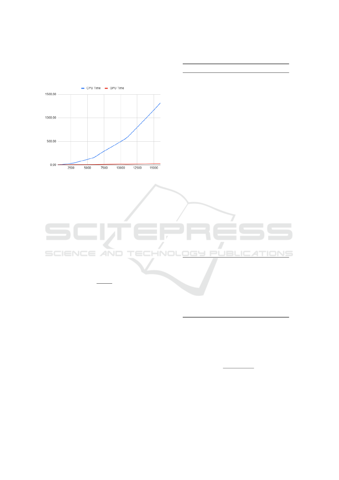
Figure 6: Execution time of CWC (blue) and CWG (red).

Figure 6 shows the execution times as a function

of the number of nodes for the CWC (blue), where the

trend is exponential, and for the CWG (red), which

remains essentially linear.

Impact of LAPR. The table 5 shows the results ob-

tained by applying the LAPR approach. The ﬁrst two

columns indicate the instance name and the number of

nodes, respectively. The next two columns are related

to the number of entries in the original savings list

Len

Ori

and those belonging to the reduced list Len

Red

The last column displays the reduction achieved, de-

termined as

% =

Len

Red

Len

Ori

× 100.

The computational results underline a substantial re-

duction. In fact, considering that each node is con-

nected with all other nodes to obtain the savings list,

each time a node is excluded, on average, entries

equal to the number of nodes are removed from the

savings list. This approach required adjusting a hy-

perparameter that deﬁnes how often nodes, present in

the tabu list, should activate the reduction procedure.

Since the merging is done on the CPU and reduction

on the GPU, each time reduction is invoked, neces-

sary overhead must be considered. Empirically, we

found that the best result is obtained by ﬁltering the

list when the tabu list contains 1,000 nodes.

Comparison with Previous Approach. Lastly, the

Tab. 6 presents a comparative analysis of perfor-

mance with the algorithm in (Guerriero and Sacco-

manno, 2024), in eight different instances, selected

Table 5: LAPR reduction of savings list.

Instance Nodes Len

Ori

Len

Red

X-n502-k39 502 125250 23696 19%

X-n513-k21 513 130816 11593 9%

X-n524-k153 524 136503 70336 52%

X-n536-k96 536 142845 46667 33%

X-n548-k50 548 149331 32120 22%

X-n561-k42 561 156520 18518 12%

X-n573-k30 573 163306 27272 17%

X-n586-k159 586 170820 102870 60%

X-n599-k92 599 178503 57547 32%

X-n613-k62 613 186966 27913 15%

X-n627-k43 627 195625 39735 20%

X-n641-k35 641 204480 25929 13%

X-n655-k131 655 213531 76920 36%

X-n670-k130 670 223446 79827 36%

X-n685-k75 685 233586 30928 13%

X-n701-k44 701 244650 37951 16%

X-n716-k35 716 255255 33764 13%

X-n733-k159 733 267546 90159 34%

X-n749-k98 749 279378 58502 21%

X-n766-k71 766 292230 49023 17%

X-n783-k48 783 305371 38183 13%

X-n801-k40 801 319600 35025 11%

X-n819-k171 819 334153 108502 32%

X-n837-k142 837 349030 105944 30%

X-n856-k95 856 365085 46315 13%

X-n876-k59 876 382375 50136 13%

X-n895-k37 895 399171 28040 7%

X-n916-k207 916 418155 176281 42%

X-n936-k151 936 436645 84975 19%

X-n957-k87 957 456490 59367 13%

X-n979-k58 979 477753 66164 14%

X-n1001-k43 1001 499500 39275 8%

Leuven1 3001 4498500 974232 22%

Leuven2 4001 7998000 1092037 14%

Antwerp1 6001 17997000 1187458 7%

Antwerp2 7001 24496500 1498080 6%

Ghent1 10001 49995000 2826278 6%

Ghent2 11001 60494500 1878885 3%

Brussels1 15001 112492500 3336386 3%

Brussels2 16001 127992000 2287755 2%

Flanders1 20001 199990000 5018038 3%

Flanders2 30001 449985000 5022633 1%

due to their large number of nodes. The columns rep-

resent the instance, the computational time in seconds

for both algorithms (T

CWG

and T

CWG

), and the per-

centage reduction in computational time when using

CWG

compared to T

CWG

, calculated as

T R

% =

CWG

− T

CWG

× 100.

CWG demonstrates a decrease in time ranging from

at least 75% to as much as 93%. Furthermore, as

the number of nodes increases, the time reduction be-

comes more signiﬁcant, highlighting the impact of the

LAPR procedure that is absent in T

CWG

. In effect,

A Parallel Implementation of the Clarke-Wright Algorithm on GPUs

109

previous research focused on assessing the viability

of running the CW algorithm on GPUs and analyz-

ing the execution times of various steps on both the

CPU and GPU. However, that study did not include

the development of the LAPR reduction method, thus

the route merging phase was quite costly due to the

large number of savings to process when dealing with

instances that have a high number of nodes.

Table 6: Comparison with (Guerriero and Saccomanno,

2024).

Instance T

CWG

T R

L1 15.21 3.75 75.35%

L2 23.40 3.49 85.09%

A1 46.78 4.83 89.68%

A2 72.30 7.57 89.53%

G1 155.66 14.18 90.89%

G2 203.80 15.87 92.21%

B1 393.24 35.69 90.92%

B2 451.05 29.95 93.36%

Average 170.18 14.42 88.38%

5 CONCLUSIONS

In this work, a CWG implementation on GPU of the

CW algorithm was proposed. The computational re-

sults collected clearly highlight that it is signiﬁcantly

faster than the CWC implementation, especially for

large instances. This is due to the parallel process-

ing capabilities of GPUs, which enable efﬁcient ex-

ecution of the computational steps of the algorithm,

leading to substantial speedups.

Comparison with a state-of-the-art PyVRP algo-

rithm, which uses the same initial data structures, in-

dicates that the GPU implementation could signif-

icantly improve the performance and scalability of

such a solver, particularly in the early stages, there-

fore suggesting a possible integration of the two ap-

proaches. Moreover, by enabling substantial accelera-

tion in the search for an initial solution, albeit not nec-

essarily optimal, this approach can be integrated into

other heuristics to quickly provide an initial solution.

It can also serve as the basis for an iterative method,

aimed at quickly exploring the solution space.

Future research could focus on extending the

applicability of GPU-accelerated CW algorithms to

more complex VRP variants and exploring their

potential for solving related optimization problems

across various domains.

For instance, it provides an effective approach for

real-time applications needing rapid, nearly optimal

vehicle routing solutions. Our ﬁndings indicate that

the algorithm consistently achieves results within a

7% gap from optimal, thus making it ideal for sce-

narios where timely decisions are essential. By utiliz-

ing the parallel processing power of GPUs, we have

accomplished notable speed enhancements, allowing

the algorithm to produce high-quality solutions in

much less time than standard CPU-based methods.

These results underscore the promise of GPU acceler-

ation in addressing complex optimization challenges

in dynamic and time-sensitive settings.

REFERENCES

Abdelatti, M. F. and Sodhi, M. S. (2020). An improved

gpu-accelerated heuristic technique applied to the ca-

pacitated vehicle routing problem. In Proceedings of

the 2020 Genetic and Evolutionary Computation Con-

ference, GECCO ’20, page 663–671, New York, NY,

USA. Association for Computing Machinery.

Accorsi, L. and Vigo, D. (2021). A fast and scalable heuris-

tic for the solution of large-scale capacitated vehicle

routing problems. Transportation Science, 55(4):832–

856.

Arnold, F., Gendreau, M., and S

orensen, K. (2019). Ef-

ﬁciently solving very large-scale routing problems.

Computers & Operations Research, 107:32–42.

Augerat, P., Belenguer, J. M., Benavent, E., Corberan, A.,

Naddef, D., and Rinaldi, G. (1995). Computational

results with a branch and cut code for the capacitated

vehicle routing problem. Computer Science, Mathe-

matics.

Benaini, A. and Berrajaa, A. (2016). Solving the dynamic

vehicle routing problem on gpu. In 2016 3rd Interna-

tional Conference on Logistics Operations Manage-

ment (GOL), pages 1–6.

Benaini, A. and Berrajaa, A. (2018). Genetic algorithm for

large dynamic vehicle routing problem on gpu. In

2018 4th International Conference on Logistics Op-

erations Management (GOL), pages 1–9.

Benaini, A., Berrajaa, A., and Daoudi, E. M. (2016).

Solving the vehicle routing problem on gpu. In

El Oualkadi, A., Choubani, F., and El Moussati, A.,

editors, Proceedings of the Mediterranean Conference

on Information & Communication Technologies 2015,

pages 239–248, Cham. Springer International Pub-

lishing.

Benaini, A., Berrajaa, A., and Daoudi, E. M. (2017). Par-

allel implementation of the multi capacity vrp on gpu.

In Rocha,

A., Serrhini, M., and Felgueiras, C., editors,

Europe and MENA Cooperation Advances in Infor-

mation and Communication Technologies, pages 353–

364, Cham. Springer International Publishing.

Bor

cinov

a, Z. (2022). Kernel search for the capacitated ve-

hicle routing problem. Applied Sciences, 12(22).

Boschetti, M. A., Maniezzo, V., and Strappaveccia, F.

(2017). Route relaxations on gpu for vehicle rout-

ing problems. European Journal of Operational Re-

search, 258(2):456–466.

ICORES 2025 - 14th International Conference on Operations Research and Enterprise Systems

110

Caccetta, L., Alameen, M., and Abdul-Niby, M. (2013). An

improved clarke and wright algorithm to solve the ca-

pacitated vehicle routing problem. Engineering, Tech-

nology & Applied Science Research, 3(2):413–415.

Clarke, G. and Wright, J. W. (1964). Scheduling of vehicles

from a central depot to a number of delivery points.

Operations research, 12(4):568–581.

Diego, F. J., G

omez, E. M., Ortega-Mier, M., and Garc

ıa-

anchez,

A. (2012). Parallel cuda architecture for

solving de vrp with aco. In Sethi, S. P., Bogataj, M.,

and Ros-McDonnell, L., editors, Industrial Engineer-

ing: Innovative Networks, pages 385–393, London.

Springer London.

Guerriero, F. and Saccomanno, F. (2024). Accelerating

the clarke-wright algorithm for the capacitated vehicle

routing problem using gpus. In Proceedings of BOS /

SOR 2024, Polish Operational and Systems Research

Society Conference, Warsaw.

Jin, J., Crainic, T. G., and Løkketangen, A. (2014). A co-

operative parallel metaheuristic for the capacitated ve-

hicle routing problem. Computers & Operations Re-

search, 44:33–41.

Laporte, G. (1992). The vehicle routing problem: An

overview of exact and approximate algorithms. Eu-

ropean Journal of Operational Research, 59(3):345–

358.

Liu, F., Lu, C., Gui, L., Zhang, Q., Tong, X., and Yuan,

M. (2023). Heuristics for vehicle routing problem: A

survey and recent advances.

Luong, T. V., Melab, N., and Talbi, E.-G. (2013). Gpu com-

puting for parallel local search metaheuristic algo-

rithms. IEEE Transactions on Computers, 62(1):173–

185.

Nurcahyo, R., Irawan, D. A., and Kristanti, F. (2023). The

effectiveness of the clarke & wright savings algorithm

in determining logistics distribution routes (case study

pt.xyz). E3S Web of Conferences, 426.

Schulz, C. (2013). Efﬁcient local search on the

gpu—investigations on the vehicle routing prob-

lem. Journal of Parallel and Distributed Computing,

73(1):14–31. Metaheuristics on GPUs.

Tunnisaki, F. and Sutarman (2023). Clarke and wright sav-

ings algorithm as solutions vehicle routing problem

with simultaneous pickup delivery (vrpspd). Journal

of Physics: Conference Series, 2421(1):012045.

Uchoa, E., Pecin, D., Pessoa, A., Poggi, M., Vidal, T., and

Subramanian, A. (2017). New benchmark instances

for the capacitated vehicle routing problem. European

Journal of Operational Research, 257(3):845–858.

Wouda, N. A., Lan, L., and Kool, W. (2024). PyVRP: a

high-performance VRP solver package. INFORMS

Journal on Computing.

Yelmewad, P. and Talawar, B. (2021). Parallel version

of local search heuristic algorithm to solve capaci-

tated vehicle routing problem. Cluster Computing,

24(4):3671–3692.

A Parallel Implementation of the Clarke-Wright Algorithm on GPUs

111