Features for Classifying Insect Trajectories in Event Camera Recordings
Regina Pohle-Fr
¨
ohlich
1 a
, Colin Gebler
1 b
, Marc B
¨
oge
1
, Tobias Bolten
1 c
, Leland Gehlen
2
,
Michael Gl
¨
uck
2 d
and Kirsten S. Traynor
2 e
1
Institute for Pattern Recognition, Niederrhein University of Applied Sciences, Krefeld, Germany
2
State Institute of Bee-Research, University of Hohenheim, Stuttgart, Germany
Keywords:
Event Camera, Classification, Insect Monitoring.
Abstract:
Studying the factors that affect insect population declines requires a monitoring system that automatically
records insect activity and environmental factors over time. For this reason, we use a stereo setup with two
event cameras in order to record insect trajectories. In this paper, we focus on classifying these trajectories
into insect groups. We present the steps required to generate a labeled data set of trajectory segments. Since
the manual generation of a labelled dataset is very time consuming, we investigate possibilities for label
propagation to unlabelled insect trajectories. The autoencoder FoldingNet and PointNet++ as a classification
network for point clouds are analyzed to generate features describing trajectory segments. The generated
feature vectors are converted to 2D using t-SNE. Our investigations showed that the projection of the feature
vectors generated with PointNet++ produces clusters corresponding to the different insect groups. Using the
PointNet++ with fully-connected layers directly for classification, we achieved an overall accuracy of 90.7%
for the classification of insects into five groups. In addition, we have developed and evaluated algorithms for
the calculation of the speed and size of insects in the stereo data. These can be used as additional features for
further differentiation of insects within groups.
1 INTRODUCTION
Many species are currently in serious decline or
threatened by extinction due to human activities that
influence populations, including habitat loss, the in-
troduction of invasive species, climate change and en-
vironmental pollution. This global decline in biodi-
versity observed in recent years is a worrying trend,
as biodiversity is essential for the functioning of all
ecosystems (Saleh et al., 2024).
Insects are particularly valuable indicators for as-
sessing changes in biodiversity, as they serve as both
a food source for many other species and, in some
cases, as pollinators of flowering plants (Landmann
et al., 2023). Efficiently monitoring the current insect
population is therefore crucial for understanding how
various stress factors impact these populations, and by
extension, biodiversity. Such systems can also evalu-
ate the effectiveness of measures designed to protect
a
https://orcid.org/0000-0002-4655-6851
b
https://orcid.org/0009-0006-4654-032X
c
https://orcid.org/0000-0001-5504-8472
d
https://orcid.org/0009-0006-9888-436X
e
https://orcid.org/0000-0002-0848-4607
insects.
Currently, monitoring is often conducted using
different types of traps (e.g., malaise traps, pitfall
traps, light traps or pen traps), which makes data anal-
ysis very labor-intensive. Fully automated monitoring
methods are needed. In addition to acoustic and radar-
based remote sensing methods, computer vision tech-
niques are gaining traction (Van Klink et al., 2024).
For example, systems have been developed that use
cameras to capture, segment, and classify insects
caught in traps ((Sittinger et al., 2024), (Tschaikner
et al., 2023)). However, these methods are limited
in that they cannot capture insect activities. When
videos are recorded within a natural enviroment, nu-
merous cameras are required to observe a larger area,
as successful segmentation and classification of in-
sects is only possible in close-up images due to the
complexity of the scenes (e.g., 10 cameras, each cov-
ering an area of 35x22 cm) (Bjerge et al., 2023). Fur-
thermore, high camera frame rates are needed to de-
tect small and fast-moving insects, which results in
very large amounts of data. Consequently, only short
video sequences are typically recorded at predefined
times (Naqvi et al., 2022), making continuous moni-
Pohle-Fröhlich, R., Gebler, C., Böge, M., Bolten, T., Gehlen, L., Glück, M. and Traynor, K. S.
Features for Classifying Insect Trajectories in Event Camera Recordings.
DOI: 10.5220/0013140100003912
Paper published under CC license (CC BY-NC-ND 4.0)
In Proceedings of the 20th International Joint Conference on Computer Vision, Imaging and Computer Graphics Theory and Applications (VISIGRAPP 2025) - Volume 3: VISAPP, pages
355-364
ISBN: 978-989-758-728-3; ISSN: 2184-4321
Proceedings Copyright © 2025 by SCITEPRESS – Science and Technology Publications, Lda.
355

toring impossible.
To address these challenges, we aim to use event
cameras (Gallego et al., 2020) for long-term moni-
toring of insects over large areas (several square me-
ters), as they offer a lot of advantages over other meth-
odes. For instance, moving objects are automatically
segmented for static mounted event cameras because
events are only generated when motion is detected
at a pixel position. This leads to smaller data sizes
and much higher temporal resolution compared to tra-
ditional frame cameras. Initial tests with this type
of sensor have already been conducted successfully
((Pohle-Fr
¨
ohlich and Bolten, 2023), (Pohle-Fr
¨
ohlich
et al., 2024), (Gebauer et al., 2024)). These previous
articles dealt mainly with the segmentation of insect
flight trajectories.
This paper discusses the further development of
this approach with respect to the classification of in-
sects into groups such as bees, butterflies, dragonflies,
etc. The main contributions are the classification of
the event point clouds (x,y,t) of insect trajectory parts
with neural networks and the derivation of the veloc-
ity and the estimation of the size of insects from stereo
data (x,y,z,t). The rest of this paper is organized as
follows. Section 2 gives an overview of related work.
Section 3 describes the steps for generating training
data. Section 4 explains the steps to classify the 3D
point clouds, the neural networks used, and the results
obtained. Section 5 presents the algorithm for speed
and size estimation from the 4D point clouds and the
results obtained. Finally, a short summary and out-
look on future work is given.
2 RELATED WORK
The classification of point clouds is based on descrip-
tors that capture their characteristic global and local
features. These features include geometric properties,
such as the spatial arrangement of neighboring points,
as well as statistical properties, like point density. Han
(Han et al., 2023) categorizes these descriptors into
two key categories: hand-crafted methods and deep
learning-based approaches. A well-designed descrip-
tor for differentiating insects based on point clouds
generated from their flight trajectory requires expert
knowledge of insect flight behavior to accurately de-
scribe the typical variations between the point clouds.
This is not available. In contrast, deep learning fea-
tures do not require specific domain knowledge; in-
stead, they rely on classified samples.
If only a limited number of classified data sets are
available, one approach is to use an autoencoder for
point clouds to learn the specific properties of the in-
dividual unclassified point cloud trajectories. Autoen-
coders are self-supervised learning methods where
the encoder transforms the point cloud into a latent
code and the decoder expands it to reconstruct the in-
put. Different network architectures can be found in
the literature, for instance MAE (Zhang et al., 2022),
IAE (Yan et al., 2023) or FoldingNet (Yang et al.,
2018). In few-shot learning, labels are assigned to
the feature space formed by a selected network layer
of the autoencoder using some labeled sample data.
An SVM can then be used, for example, to classify
unknown data (Ju et al., 2015).
However, the feature space can also be compacted
before classification using dimension reduction meth-
ods. Benato has shown in (Benato et al., 2018) that
using a 2D t-SNE projection for this purpose often
provides more accurate labels than direct propagation
in the feature space.
If more data sets of labeled point clouds are avail-
able, neural networks can also be used for direct clas-
sification. In this case, the features are learned in
such a way that optimal class discrimination is pos-
sible. Several deep learning approaches can be used
for event point clouds, such as voxel-based methods,
methods based on multi-view representations, point-
based approaches, and graph-based methods (Han
et al., 2023). Point-based methods achieve state-of-
the-art results. A disadvantage compared to the other
approaches is that they only work with a small fixed
number of points as input, so they cannot be used to
classify the entire insect trajectory. However, they
can be used well for individual sections. A frequently
used network in the category of point-based methods
is PointNet++, which has already been successfully
used for the classification of event camera data. For
example, Bolten used it to classify objects on a pub-
lic playground (e.g. people, bicycle, dog, bird, in-
sect, rain, shadow, etc.) in the DVS-OUTLAB data
set (Bolten et al., 2022) and Ren used it for action
classification in the DVS128 gesture data set (Ren
et al., 2024). Compared to other point-based net-
works, one advantage is that PointNet++ requires a
comparatively small number of parameters.
3 DATA SET PREPARATION
A large number of training data, ideally several hun-
dred insect trajectories per class, is needed to train
the neural networks. Currently, there are no publicly
available labeled event-based data sets for this appli-
cation area. Therefore, the training material had to be
created in-house. Our data set is based on four differ-
ent data sources:
VISAPP 2025 - 20th International Conference on Computer Vision Theory and Applications
356

• Data Set of the University of M
¨
unster. This data
set (Gebauer et al., 2024) contains 13 minutes of
DVS and RGB recordings of 6 scenes. It con-
tains only bees or unidentifiable insects. In ad-
dition, the DVS recordings are available as con-
verted videos, as well as CSV files describing the
positions and sizes of the bounding boxes within
the video frames. A confidence value indicates
whether the annotator was sure that the bounding
box contained an insect or not.
• HSNR Data Set. The data set contains 132 min-
utes of pre-segmented DVS recordings from 6
scenes (Pohle-Fr
¨
ohlich et al., 2024). It contains
bees, butterflies, dragonflies and wasps. Annota-
tions for the individual flight trajectories are not
available.
• Combination of Event Camera and Frame
Camera Recordings. To supplement the avail-
able data, we recorded our own event streams us-
ing an event camera with a IMX636 HD sensor
distributed by Prophesee together with a Rasp-
berry Pi global RGB shutter camera with a Sony
IMX296 sensor. The simultaneous video streams
allowed later assignment of flight trajectories to
individual insect groups.
• Stereo Event Camera Data. Stereo event data
were required for some experiments. These
were recorded using the stereo setup described in
(Pohle-Fr
¨
ohlich et al., 2024). Insects were caught
with a butterfly net and later released in front of
the cameras. This provides flight trajectories for
which the species is known.
In later long-term monitoring, the individual trajec-
tories will be extracted automatically using instance
segmentation together with an object tracking algo-
rithm. As these are still being developed, the various
data sources had to be processed manually for this
work in order to obtain a labeled data set with dif-
ferent insect trajectories.
3.1 Assignment of Insect Class
To label the data, the HSNR datasets and the datasets
recorded specifically for this study are converted to
a frame representation by projecting events and saved
in a video with a frame rate of 60 fps. Bounding boxes
are then drawn around the individual insects using
the labeling software DarkLabel
1
, where an instance
ID is automatically generated. Manual assignment to
an insect group is also carried out (Figure 1). For
the data from the University of M
¨
unster, where the
1
https://github.com/darkpgmr/DarkLabel
Table 1: Number of trajectories with mean event number
and mean length per insect group in the combined data set.
Insect Trajec- Mean Mean Total
group tory event length length
count count in s in s
Honey bee 66 35268.95 5.53 364.97
Bumble bee 47 72270.32 1.14 53.62
Wasp 83 12602.16 1.19 98.76
Butterfly 21 109321.71 5.01 105.17
Dragonfly 112 52047.11 1.88 210.17
bounding boxes are already available, self-developed
software is used to assign an instance ID and an insect
group to each bounding box.
3.2 Trajectory Extraction
The next step is to extract the trajectories of each in-
stance. The point cloud of a trajectory consists of all
events within the insect’s bounding boxes. Since the
bounding boxes are created on the videos, they have
a position (x, y), a dimension (width and height), and
a frame index. To reduce the stepping effect between
adjacent frames, intermediate bounding boxes are in-
serted by interpolating the coordinates of two adja-
cent bounding boxes during processing. The result
is shown in Figure 2 for an example trajectory of a
bee. All extracted trajectories are then normalized so
that the centroid of the point cloud is at the origin of
the coordinates and all points are within radius of 1,
where the time t in microseconds is previously multi-
plied by 0.002 in order to balance the different scales.
Table 1 shows the number of extracted complete tra-
jectories per insect group with the mean event count
and mean length. The data set is available at the fol-
lowing link https://github.com/Event-Based-Insects/
VISAPP25-DVS-Insect-Classification.
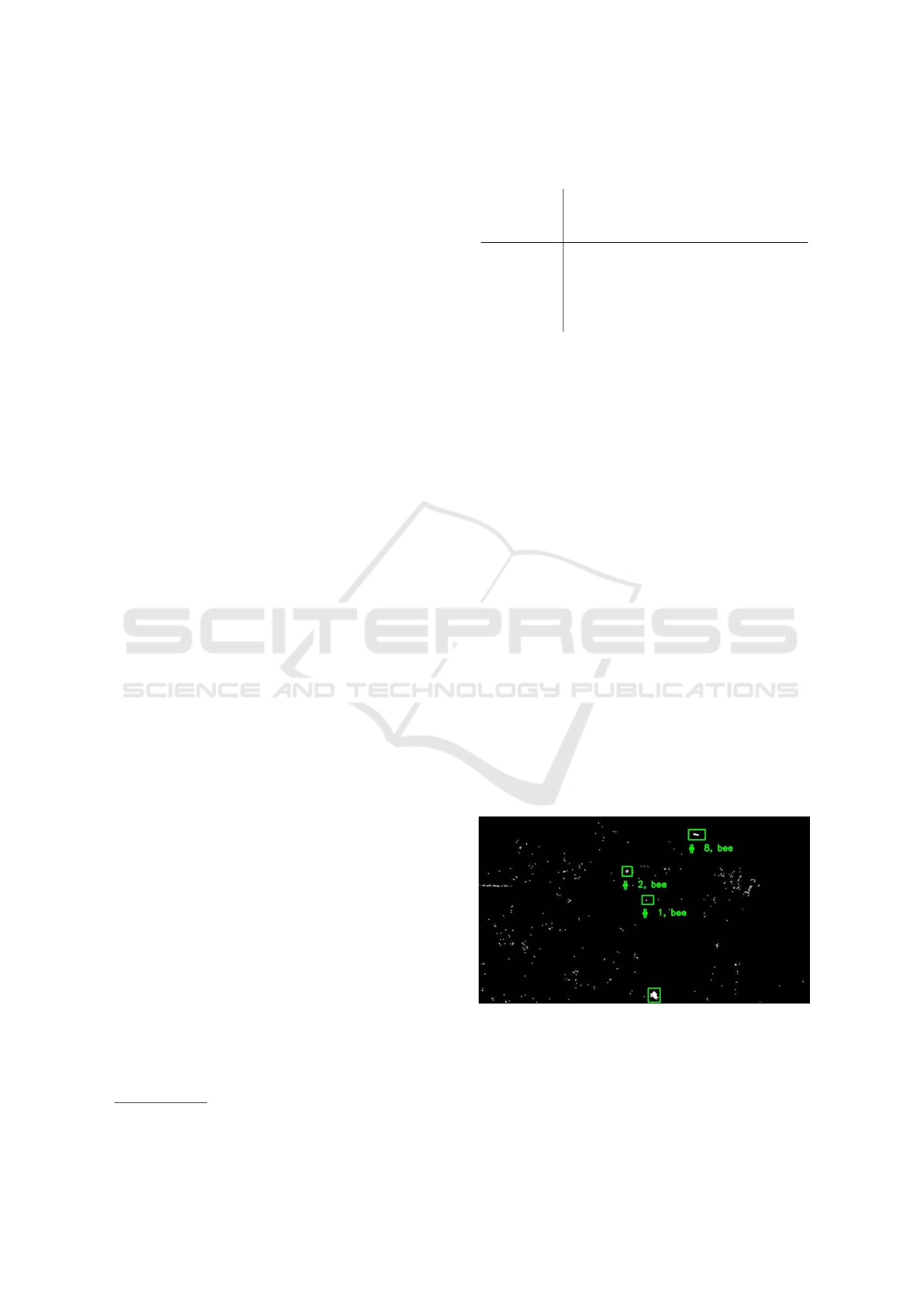
Figure 1: Example frame with the manually marked bound-
ing boxes of the bees contained in the frame.
Features for Classifying Insect Trajectories in Event Camera Recordings
357

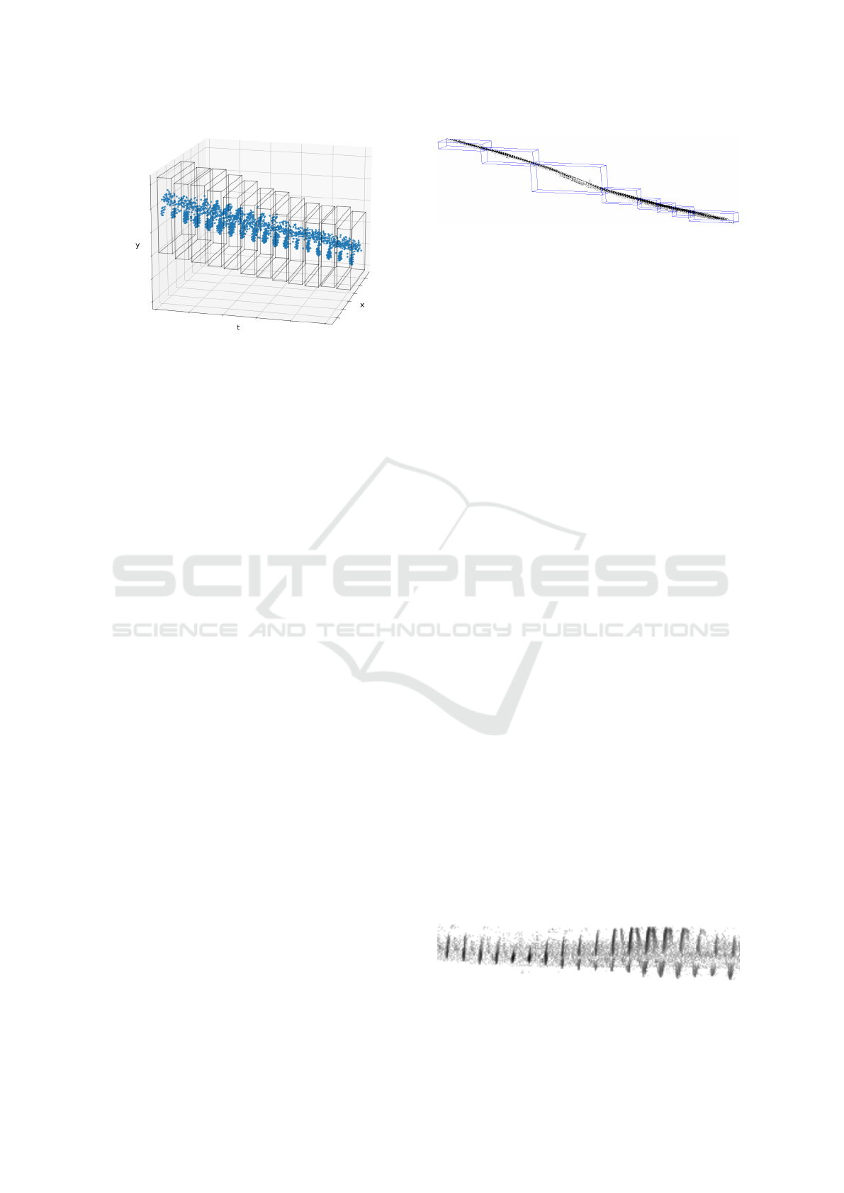
Figure 2: Extracted example flight path for a bee resulting
from the semi-automatically marked bounding boxes in the
corresponding video frames.
3.3 Selection of the Point Cloud Parts
To use the trajectories as input for point-based neural
networks, they need a fixed number of points. For our
study, we use 4096 points as the input size. There are
several ways to modify or decompose the trajectories
to achieve the target number of points.
• Using the Complete Extracted Trajectory. If
we take the point cloud of a complete flight tra-
jectory, in most cases we have to downsample
considerably, because flight trajectories of insects
closer to the camera can have more than a million
points. All the fine details, such as wing beats,
would be lost by down sampling. In addition, the
trajectories vary in time from a few hundred mil-
liseconds to over 20 seconds. This also leads to
distortions in the input data.
• Splitting the Trajectory into Parts with Equal
Point Count. If the trajectories are divided into
segments with a fixed number of points, this has
the advantage that no up- or downsampling is re-
quired and therefore no data loss occurs. The tem-
poral length of the fragments then depends di-
rectly on the number of points or point density
at the location of the part. The problem is that
the point density of the trajectories varies signifi-
cantly depending on the size of the insect, the dis-
tance to the camera, the velocity and the wing beat
frequency of the wings, as shown in the example
in Figure 3. In extreme cases, when insects fly
close to the camera, only a single wing beat fits
into the time window. As a result, the data are not
comparable.
• Splitting the Trajectory into Parts of Fixed Du-
ration. Fragments that are easier to compare can
be obtained by dividing the flight trajectories into
parts with a constant time interval. In this way,
Figure 3: Example of a bee trajectory divided into segments
of 4096 points each. The different point densities result in
segments of different lengths.
depending on the insect species, roughly the same
number of wing beats always fit into a fragment,
and the neural networks can better learn to recog-
nize the corresponding patterns. This raises the
challenge of selecting a time window that enables
optimal discrimination. Rough flight patterns can
be captured by selecting time windows of a few
seconds. However, this leads to the problem that
downsampling may be necessary, which can lead
to the loss of information. Another problem is
that shorter sections cannot be classified at all.
For this reason, in this study we decided to di-
vide the trajectories into short sections to allow
the recognition of the individual wing beats. Ex-
periments have shown that a time window of 100
ms is suitable for solving our problem. For insects
with a low wing beat frequency, e.g. butterflies,
an average of about 1.5 wing beats are recorded
in this time window. For insects with a higher
wing beat frequency, such as bees, the extracted
segment contains about 20 wing beats (Figure 4).
3.4 Noise Reduction and Sampling
Statistical outlier removal is used for noise reduc-
tion, which removes points whose distance to their
nearest 40 neighbors is greater than the 6 times the
standard deviation in the point cloud. An advantage
of this method is that it is data dependent and can
deal with point clouds of different densities. After
noise filtering, the point cloud must be sampled up or
down. All segments with less than 2048 points are
discarded as unclassifiable because the data do not
contain sufficient insect-specific information. Such
trajectories are generated, for example, when insects
fly at a greater distance from the camera, or when they
pass behind a plant. Upsampling is performed for all
Figure 4: t-y projection of a 100ms time interval of a bee
trajectory; t-scaling = 0.002.
VISAPP 2025 - 20th International Conference on Computer Vision Theory and Applications
358

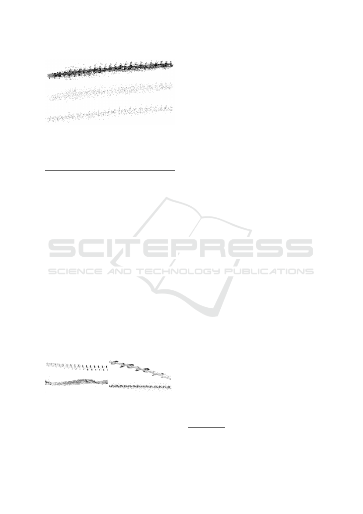
Figure 5: Comparison of original point cloud with 64.201
points (top) farthest point sampling (middle) and random
sampling (bottom) for a bee trajectory of a 100ms time in-
terval.
Table 2: Number of trajectories n for the three categories.
Insect group n < 2048 2048 ≤ n ≤ 4096 n > 4096
Honey bee 3368 194 123
Bumble bee 214 100 224
Wasp 925 66 30
Butterfly 844 133 80
Dragonfly 1261 470 397
segments with a event count between 2048 and 4096
points by doubling randomly selected points until a
number of 4096 is reached. For the downsampling of
point clouds with more than 4096 points, we investi-
gated random and farthest point sampling. A visual
comparison (Figure 5) shows that the random sam-
pled structure retained more details when a large re-
duction in the number of points was necessary. How-
ever, as such extreme point reduction was very rare,
and we achieved better classification results with the
farthest point sampling, we used it to learn the fea-
tures. Table 2 shows the number of segments per
group of insects for the three categories. The num-
ber of segments of both groups with more than 2048
points each can be used for classification. The high
proportion of bee flight paths with less than 2048
points compared to butterflies or dragonflies is due
to the fact that bees are relatively small and are of-
ten temporarily covered by grasses when collecting
pollen in a meadow. Figure 6 illustrates examples of
trajectory segments from various insects.
Figure 6: Flight pattern of bee (top left), butterfly (bottom
left), dragonfly (top right) and wasp (bottom left).
3.5 Selection of Trajectory Parts
In the later application, the segment used to classify
the entire trajectory is selected depending on the ob-
ject depth. For this purpose, the trajectory is divided
into individual segments of 100 ms and the average z-
coordinate is calculated. The segment with the short-
est distance to the camera is used, since it has the
highest level of detail. For our test application, the
segments are manually selected.
4 DEEP-LEARNING BASED
DESCRIPTORS
To characterize the insect flight patterns, features
were investigated by training an autoencoder as well
as a classification network. For both neural networks,
the data set was split in a ratio of 70:30 into a training
data set and a test data set. It was taken into account
that the segments of all classes were divided in this
ratio and that all segments of a single insect’s flight
trajectory were assigned to either the training or the
test data set.
4.1 Autoencoder
In our investigations, we use FoldingNet (Yang et al.,
2018) as an autoencoder specifically designed for
point clouds. The encoder is graph-based, which
means that local structures are better taken into ac-
count. Subsequently, a folding-based decoder trans-
forms a canonical 2D grid into the underlying 3D ob-
ject surface of a point cloud. The advantage of this
decoder is that it requires only a very small number
of parameters compared to a fully connected decoder.
For our experiments, we used the implementation pro-
vided by the developers
2
, but used our chosen num-
ber of 4096 points. We also used 1024 feature dimen-
sions and started from a Gaussian distributed point
cloud (Figure 7). Due to the small amount of training
data, we used dropout and considered 40 neighbors
for kNN sampling. As data augmentation, we used
random rotate and translate and limited jitter. Train-
ing was done for 1200 epochs with a batch size of
16. All segments of the whole data set were used for
training. This is not a problem here, because only the
point clouds without class labels are used for recon-
struction. Figure 7 shows an example of a dragonfly’s
original point cloud and the result of the autoencoder
reconstructed point cloud. The FoldingNet manages
2
https://github.com/antao97/
UnsupervisedPointCloudReconstruction
Features for Classifying Insect Trajectories in Event Camera Recordings
359

to align the point clouds, but it is clear to see that a lot
of detail is lost from the flight patterns. We later ex-
amined the output of the trained encoder as a feature
vector for classifying the trajectories.
4.2 PointNet++
PointNet++ (Qi et al., 2017) can be used to classify
point cloud data. In this context, the input data is
first hierarchically subdivided and summarized. This
is achieved through a sequence of set abstraction lay-
ers. In each layer, a set of points is processed and
abstracted, resulting in a new set with fewer points
but more features. Each set abstraction layer consists
of three layers, a Sampling layer, a Grouping layer,
and a PointNet layer. The Sampling layer selects a
subset of points with approximately equal distances
from the set of points using farthest point sampling.
These points represent the centroids of the following
layer. The points of the entire set are then grouped
by these centroids in the Grouping layer. Finally, a
feature vector is generated for each group using the
PointNet layer. This describes the features of the local
neighborhood of a group. For the hierarchical appli-
cation of the set abstraction layers, we use the multi-
scale grouping proposed by Qi and the implementa-
tion provided by the PyTorch library
3
. We trained a
three-level hierarchical network with three fully con-
nected layers for 40 epochs with a batch size of 8. We
used the Adam algorithm as optimizer with a learning
rate of 0.001 and a weight decay of 0.0004. All other
parameters are set to their default values. The code of
the network was additionally extended for our task so
that the feature vectors could be output after the sec-
ond Fully Connected layer during feed forwarding.
4.3 Results of Trajectory Classification
Figure 8 shows the t-SNE projection of the segment
feature vectors of the trained FoldingNet with its best
result. In the visualization, no distance-based clusters
Figure 7: Reconstructed point clouds of a dragonfly flight
trajectory after different numbers of training epochs a) 0, b)
20, c) 40, d) 100, e) 1200 epochs and f) the original point
cloud for comparison.
3
https://github.com/yanx27/Pointnet Pointnet2 pytorch
can be recognized. Only coarse, color-differentiated
regions are visible. For example, bees (orange) tend
to cluster in the center, while dragonflies (blue) are
scattered to the left and right. Several small clusters
of wasps (yellow) are present at the very edge. The
poor results are mainly due to the fact that the re-
constructed point clouds show a high loss of detail,
as shown in Figure 7. As a result, the use of this
approach in combination with an SVM for few-shot
learning is not promising.
The PointNet++ delivered better results. We
achieved an overall accuracy of 90.7%. Figure 10
shows the corresponding confusion matrix indicat-
ing which groups were misclassified and how of-
ten. Dragonflies are classified most reliably. Bum-
ble bees and honey bees also have a high accuracy,
but are sometimes mixed up with each other. Butter-
flies are often recognized as dragonflies, as the data
set also contains dragonflies with a fluttering flight.
Figure 9 shows the t-SNE projection of the learned
features, with the color saturation indicating how con-
fident the PointNet++ was in the group assignment.
The features of each group have compact clusters,
which had an impact on the accuracy of group assign-
ment. Although the different groups contain different
species, e.g. the dragonfly group contains Anax im-
perator, Cordulia aenea, Enallagma cyathigerum and
Calopteryx splendens, they form a relatively compact
cluster based on the flight patterns. This approach
provides promising results and should be further in-
vestigated to learn more insect groups. It is expected
that a few-shot learning in the form of label propaga-
tion, as proposed in (Benato et al., 2018), can be used
for this purpose. A subdivision of the current groups
into subgroups, e.g. the butterfly group into different
subspecies, can be achieved by adding further charac-
teristics.
5 VELOCITY AND SIZE
ESTIMATION
In addition to flight patterns, insects can also be dis-
tinguished by their speed and size. Both of these char-
acteristics can also be used for insect tracking. To cal-
culate the velocity and size of the insect, the 3D posi-
tion of the insect in the scene must be known. For this
purpose, the stereo data set must be calibrated. This
is done as described in (Muglikar et al., 2021) using
the simulated grayscale images of the calibration pat-
terns. The depth for all events within the considered
trajectory segment can then be calculated by perform-
ing Block Matching (Konolige, 1998) on the Linear
Time Surfaces (Pohle-Fr
¨
ohlich et al., 2024) generated
VISAPP 2025 - 20th International Conference on Computer Vision Theory and Applications
360

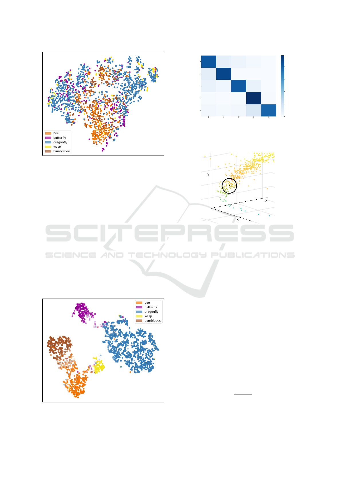
Figure 8: t-SNE projection of the feature vectors of all
training and testing segments of the FoldingNet.
from each event cameras’ respective event stream.
5.1 Algorithm for Velocity Calculation
To calculate the velocity, all neighbors within a radius
are searched for each event. From these, the event
with the largest time stamp is selected (see red point in
Figure 11). The velocity v is then calculated by divid-
ing the Euclidean distance between the two events by
the difference in time stamps. To ensure that the lin-
ear relationship can be used as a basis for calculating
the velocity, the radius must not be too large. In our
experiments, a radius of 5 cm proved to be suitable.
If the radius chosen is too large, the insect may have
flown a curve and the Euclidean distance with which
the speed is calculated may lead to an overestimation
of the speed. Figure 12 shows the connecting lines
between the events of an insect trajectory and the se-
Figure 9: t-SNE projection of the feature vectors of all
training and testing segments of the PointNet++.
bee bumble bee
wasp
dragonfly butterfly
Classification
honey bee
bumble bee
wasp
dragonfly
butterfly
Ground-Truth
0.83
0.095
0.053 0.021 0
0.1
0.9
0 0 0
0.071 0.036 0.82 0.071 0
0.0077 0 0.0077
0.98
0.0038
0.032 0.016 0.032 0.14 0.78
0.0
0.2
0.4
0.6
0.8
Figure 10: Confusion matrix for PointNet++. Rows indicate
the true class and columns the predicted class.
Figure 11: Illustration of the velocity calculation proce-
dure. The point cloud has been colored according to the
time stamp. Earlier time stamps are blue, later time stamps
are yellow. For the given black point, the red point would
be selected as the furthest point with the largest time stamp
for the given radius.
lected most distant points within the respective radius.
It is obvious that, for the selected radius, meaningful
combinations of points are also determined when fly-
ing through a curve, which allow a correct estimate of
the distance flown in a certain time window.
5.2 Algorithm for Size Estimation
In order to estimate the size of an object, it is neces-
sary to determine the accumulation time that will en-
sure a correct representation in the image for a given
object velocity. In addition to the velocity calculation
described in the previous section, the resolution of the
camera at the given object distance must also be de-
termined. For this purpose, the average distance ¯z in
mm of the insect to the camera and the average ve-
locity ¯v in m/s over the considered 100 ms period are
calculated. The number of pixels per meter n is then
n =
f · 1000
¯z
(1)
Features for Classifying Insect Trajectories in Event Camera Recordings
361

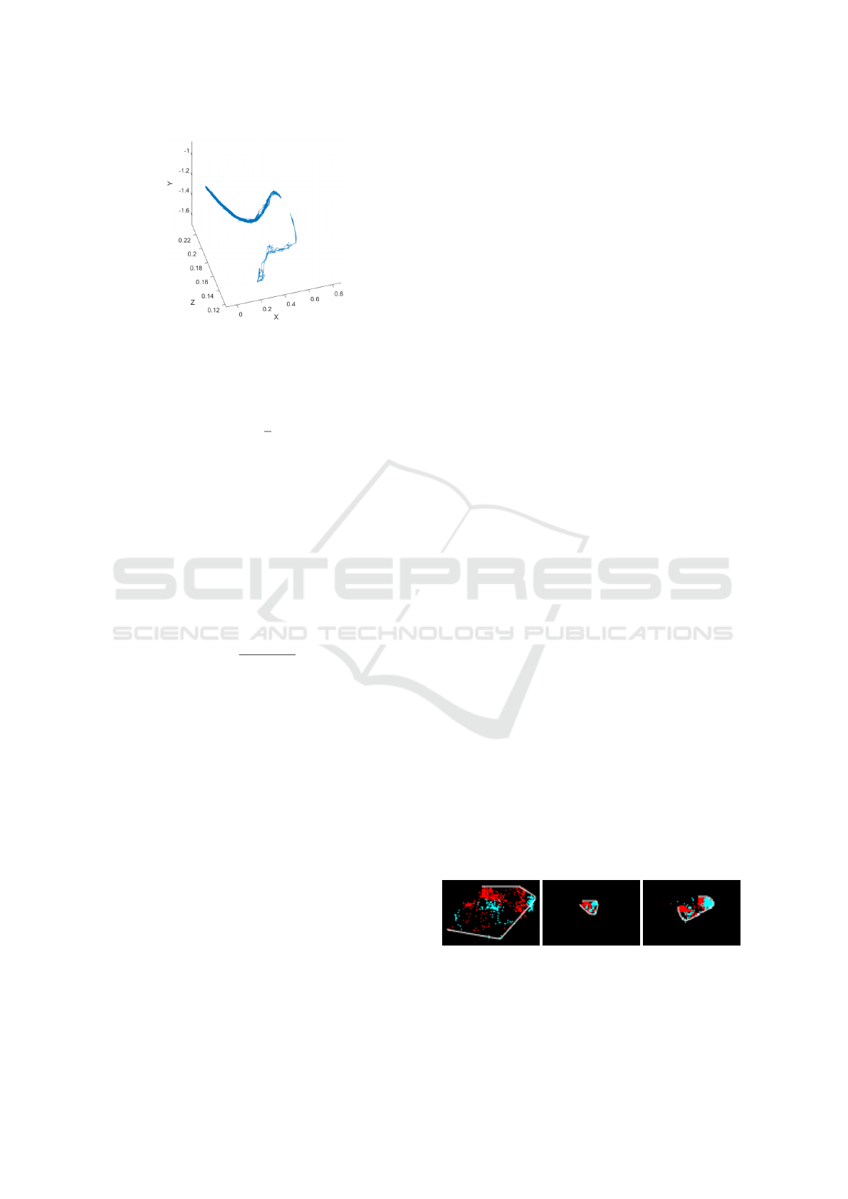
Figure 12: Distances for calculating speed, shown as lines
between an event and the corresponding farthest event
within the radius for an insect flying around the curve.
where f is the focal length. The size of a pixel s is
then calculated as
s =
1
n
(2)
Because the accepted error in size estimation should
be as small as possible, we accept a shift of the object
by 2 pixels when determining the accumulation time.
A shift of only 1 pixel would result in too few events
to identify the object. This results in an estimation
error of 2.8 mm for an insect at a distance of approx-
imately 1 m and an error of 1.6 mm for an insect at a
distance of approximately 60 cm. Since this error is
known, the result can be corrected by subtracting it.
The accumulation time t in milliseconds can then be
calculated using the following equation
t =
s · 2 · 1000
¯v
(3)
All trajectory segments that lie within the determined
accumulation time are then successively projected
onto an image. Examples are shown in Figure 13
for a honey bee, a bumble bee and a dragonfly. To
estimate the size, the extreme points of the insect re-
gion extracted per determined accumulation time are
calculated. From these points, the width and length of
the object are calculated using the Euclidean distance
between the leftmost and rightmost points and the top
and bottom points. The size is the smaller of the two,
since the larger value includes the wingspan. The size
is then multiplied by the determined pixel size s. Fi-
nally, the median values of all the determined sizes
of a trajectory is calculated to obtain the size of the
insect.
5.3 Results of Velocity and Size
Estimation
The algorithm for the calculation of the velocity has
been evaluated on stereo data of captured and released
insects as well as on the HSNR data set with data
from a meadow. In the recordings of a released honey
bee, the speed starts at 1 km/h for the first time pe-
riod analyzed. Over time, the speed increases for
each subsequent time interval until 5 km/h is reached
and the bee leaves the field of view. These calcu-
lated values are plausible. Similar results were also
obtained for the plausibility checks of the recordings
of a meadow. Figure 14 shows a 42 ms section with
an insect accelerating with increasing altitude and a
butterfly. The measured speed of the butterfly is be-
tween 4 and 10 km/h, which is in agreement with the
literature (Le Roy et al., 2019). Figure 15 shows a
section of 148 ms with an insect flying a curve. It can
be clearly seen that the flight speed slows down as it
flies through the curve. This corresponds to the mea-
surements in (Mahadeeswara and Srinivasan, 2018).
When using velocity as a characteristic to distin-
guish insect groups, altitude must also be taken into
account, as insects fly more slowly when foraging
than when flying over a meadow, as can be seen in
Figure 16 for a population of honey bees, bumble
bees and wild bees.
In addition to classification, velocity can also be
used as a criterion for connecting interrupted trajec-
tories, e.g. when an insect flies to a flower for polli-
nation and there is an interruption in the event stream
at this point. If a trajectory ends at an xy-coordinate
with a low velocity and a short time later a new trajec-
tory starts at the nearby same xy-coordinate, also with
a low velocity, it is very likely that the insect paused
on the flower. However, if a trajectory ends at a high
velocity, the insect has flown out of the camera’s field
of view or become obstructed.
The calculated velocities were also used as the ba-
sis for the size calculation algorithm. The size val-
ues of the captured and later released insects from
the stereo data are shown in Table 3. With the ex-
ception of the dragonflies, the values are within the
expected range. Because of their slender shape, per-
spective distortion has a particularly strong effect on
size estimation, resulting in particularly large varia-
tions for individual insects. As can be seen in Figure
13, it is often the case that only the wing beat width
can be measured and the length of the dragonfly is lost
Figure 13: Accumulated images of a honey bee in a dis-
tance of 17 cm (left), of a bumble bee (center) in a distance
of 1 m (right) and of a dragonfly in a distance of 80 cm. The
color represents the polarity and the white line is the con-
nection between the extrema points.
VISAPP 2025 - 20th International Conference on Computer Vision Theory and Applications
362

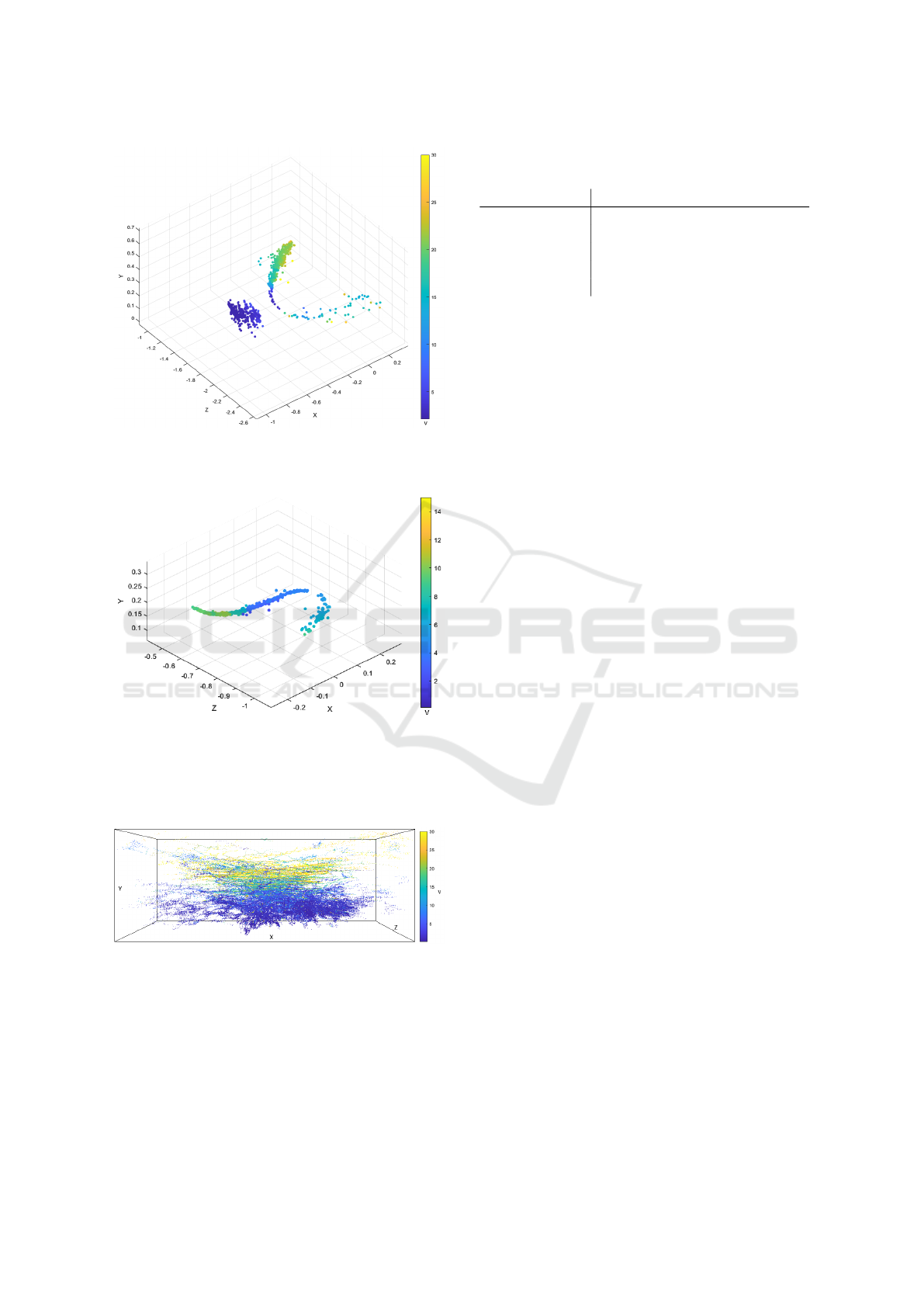
Figure 14: Calculated flight velocity in km/h of a butterfly
(left) and another insect (right) in a 42 ms section recorded
in a meadow.
Figure 15: Calculated flight speed in km/h of an insect
flying around a curve in a 148 ms section recorded in a
meadow. To calculate the speed for an event, the distances
between the corresponding points, shown as a line in the fig-
ure 12, and the corresponding difference in the time stamps
were used.
Figure 16: xy-projection of the overflights of bees and bum-
blebees in a period of 42 min with a color coding of the
flight velocity in km/h.
in the image. In this case it would be useful to choose
a different perspective from above.
Table 3: Determined size of the insects and reference value
in mm (Gerhardt and Gerhardt, 2021).
Insect name Mean size Min Max Ref.
honey bee 13.7 ± 1.9 11.5 17.2 12-16
carder bee 15.4 ± 1.1 13.3 16.7 9-17
cabbage butterfly 47.5 ± 5.7 41.8 53.3 40-65
dragonfly 21.7 ± 0.6 21.2 22.3 30-80
hoverfly 9.6 ± 0.3 9.3 9.9 5-20
6 CONCLUSIONS AND FUTURE
WORK
This paper presents three different methods that can
be used to classify insect trajectories from an event
camera into insect groups. The classification of the
point clouds of 100 ms segments of the trajectory
using PointNet++ yields very good results. This is
discernable by the clustering of the learned feature
vectors, which is clearly visible in the 2D projec-
tion generated by t-SNE. As manual labelling of data
sets is very time-consuming, this combination of fea-
ture learning on a few data sets and t-SNE projec-
tion should also be used for label propagation to other
new data. The distance of the insect from the camera
at which this differentiation is successful remains to
be investigated. Speed and size can be used to fur-
ther differentiate insects within a group. While the
speed calculation gives very reliable results, there are
still deviations between calculated and actual size de-
pending on the insect group. It will be investigated
whether a different orientation of the camera, more
from above, will give better results.
Furthermore, we plan to integrate the developed
feature calculation and the classification of insect tra-
jectories based on it into our overall system and then
evaluate this system, including automatic instance
segmentation and insect tracking, in a long-term ex-
periment.
In this experiment, the month of recording will
be taken into account as an additional parameter to
differentiate insects within a group, as some species
only occur in certain time windows. In addition to the
classification of selected segments, we plan to analyse
the entire flight curve after successful tracking, as this
varies from insect to insect within a group. For ex-
ample, it has been shown that the ratio between glid-
ing and flapping phases varies greatly among butterfly
species due to differences in wing morphology. Stud-
ies have also shown that palatable butterflies generally
fly faster and more unpredictably, while non-palatable
species fly slower and more predictably (Le Roy et al.,
2019).
Features for Classifying Insect Trajectories in Event Camera Recordings
363

ACKNOWLEDGEMENTS
This work was supported by the Carl-Zeiss-
Foundation as part of the project BeeVision.
REFERENCES
Benato, B. C., Telea, A. C., and Falc
˜
ao, A. X. (2018). Semi-
supervised learning with interactive label propagation
guided by feature space projections. In 2018 31st SIB-
GRAPI Conference on Graphics, Patterns and Images
(SIBGRAPI), pages 392–399. IEEE.
Bjerge, K., Alison, J., Dyrmann, M., Frigaard, C. E., Mann,
H. M., and Høye, T. T. (2023). Accurate detection and
identification of insects from camera trap images with
deep learning. PLOS Sustainability and Transforma-
tion, 2(3):e0000051.
Bolten, T., Lentzen, F., Pohle-Fr
¨
ohlich, R., and T
¨
onnies,
K. D. (2022). Evaluation of deep learning based
3d-point-cloud processing techniques for semantic
segmentation of neuromorphic vision sensor event-
streams. In VISIGRAPP (4: VISAPP), pages 168–179.
Gallego, G., Delbr
¨
uck, T., Orchard, G., Bartolozzi, C.,
Taba, B., Censi, A., Leutenegger, S., Davison, A. J.,
Conradt, J., Daniilidis, K., et al. (2020). Event-based
vision: A survey. IEEE transactions on pattern anal-
ysis and machine intelligence, 44(1):154–180.
Gebauer, E., Thiele, S., Ouvrard, P., Sicard, A., and Risse,
B. (2024). Towards a dynamic vision sensor-based
insect camera trap. In Proceedings of the IEEE/CVF
Winter Conference on Applications of Computer Vi-
sion, pages 7157–7166.
Gerhardt, E. and Gerhardt, M. (2021). Das große BLV
Handbuch Insekten:
¨
Uber 1360 heimische Arten,
3640 Fotos. GR
¨
AFE UND UNZER.
Han, X.-F., Feng, Z.-A., Sun, S.-J., and Xiao, G.-Q. (2023).
3d point cloud descriptors: state-of-the-art. Artificial
Intelligence Review, 56(10):12033–12083.
Ju, Y., Guo, J., and Liu, S. (2015). A deep learning method
combined sparse autoencoder with svm. In 2015 in-
ternational conference on cyber-enabled distributed
computing and knowledge discovery, pages 257–260.
IEEE.
Konolige, K. (1998). Small vision systems: Hardware and
implementation. In Shirai, Y. and Hirose, S., editors,
Robotics Research, pages 203–212. Springer.
Landmann, T., Schmitt, M., Ekim, B., Villinger, J., Ash-
iono, F., Habel, J. C., and Tonnang, H. E. (2023). In-
sect diversity is a good indicator of biodiversity sta-
tus in africa. Communications Earth & Environment,
4(1):234.
Le Roy, C., Debat, V., and Llaurens, V. (2019). Adaptive
evolution of butterfly wing shape: from morphology
to behaviour. Biological Reviews, 94(4):1261–1281.
Mahadeeswara, M. Y. and Srinivasan, M. V. (2018). Coor-
dinated turning behaviour of loitering honeybees. Sci-
entific reports, 8(1):16942.
Muglikar, M., Gehrig, M., Gehrig, D., and Scaramuzza, D.
(2021). How to calibrate your event camera. In Pro-
ceedings of the IEEE/CVF conference on computer vi-
sion and pattern recognition, pages 1403–1409.
Naqvi, Q., Wolff, P. J., Molano-Flores, B., and Sperry, J. H.
(2022). Camera traps are an effective tool for monitor-
ing insect–plant interactions. Ecology and Evolution,
12(6):e8962.
Pohle-Fr
¨
ohlich, R. and Bolten, T. (2023). Concept study
for dynamic vision sensor based insect monitoring. In
VISIGRAPP (4): VISAPP, pages 411–418.
Pohle-Fr
¨
ohlich, R., Gebler, C., and Bolten, T. (2024).
Stereo-event-camera-technique for insect monitoring.
In VISIGRAPP (3): VISAPP, pages 375–384.
Qi, C. R., Yi, L., Su, H., and Guibas, L. J. (2017). Point-
net++: Deep hierarchical feature learning on point sets
in a metric space. Advances in neural information pro-
cessing systems, 30.
Ren, H., Zhou, Y., Zhu, J., Fu, H., Huang, Y., Lin, X.,
Fang, Y., Ma, F., Yu, H., and Cheng, B. (2024). Re-
thinking efficient and effective point-based networks
for event camera classification and regression: Event-
mamba. arXiv preprint arXiv:2405.06116.
Saleh, M., Ashqar, H. I., Alary, R., Bouchareb, E. M.,
Bouchareb, R., Dizge, N., and Balakrishnan, D.
(2024). Biodiversity for ecosystem services and sus-
tainable development goals. In Biodiversity and Bioe-
conomy, pages 81–110. Elsevier.
Sittinger, M., Uhler, J., Pink, M., and Herz, A. (2024). In-
sect detect: An open-source diy camera trap for auto-
mated insect monitoring. Plos one, 19(4):e0295474.
Tschaikner, M., Brandt, D., Schmidt, H., Bießmann, F.,
Chiaburu, T., Schrimpf, I., Schrimpf, T., Stadel, A.,
Haußer, F., and Beckers, I. (2023). Multisensor data
fusion for automatized insect monitoring (kinsecta).
In Remote Sensing for Agriculture, Ecosystems, and
Hydrology XXV, volume 12727. SPIE.
Van Klink, R., Sheard, J. K., Høye, T. T., Roslin, T.,
Do Nascimento, L. A., and Bauer, S. (2024). To-
wards a toolkit for global insect biodiversity monitor-
ing. Philosophical Transactions of the Royal Society
B, 379(1904):20230101.
Yan, S., Yang, Z., Li, H., Song, C., Guan, L., Kang, H.,
Hua, G., and Huang, Q. (2023). Implicit autoencoder
for point-cloud self-supervised representation learn-
ing. In Proceedings of the IEEE/CVF International
Conference on Computer Vision, pages 14530–14542.
Yang, Y., Feng, C., Shen, Y., and Tian, D. (2018). Fold-
ingnet: Point cloud auto-encoder via deep grid defor-
mation. In Proceedings of the IEEE conference on
computer vision and pattern recognition, pages 206–
215.
Zhang, R., Guo, Z., Gao, P., Fang, R., Zhao, B., Wang, D.,
Qiao, Y., and Li, H. (2022). Point-m2ae: multi-scale
masked autoencoders for hierarchical point cloud pre-
training. Advances in neural information processing
systems, 35:27061–27074.
VISAPP 2025 - 20th International Conference on Computer Vision Theory and Applications
364