Separation of Insect Trajectories in Dynamic Vision Sensor Data

Juliane Arning, Christoph Dalitz

and Regina Pohle-Fr

ohlich

Institute for Pattern Recognition, Niederrhein University of Applied Sciences, Reinarzstr. 49, Krefeld, Germany

Keywords:

Event Camera, Clustering, Insect Monitoring.

Abstract:

We present a method to separate insect ﬂight trajectories in dynamic vision sensor data and for their math-

ematical description by smooth curves. The method consists of four steps: Pre-processing, clustering, post-

processing, and curve ﬁtting. As the time and space coordinates use different scales, we have rescaled the

dimensions with data-based scale factors. For clustering, we have compared DBSCAN and MST-based clus-

tering, and both suffered from undersegmentation. A suitable post-processing was introduced to ﬁx this. Curve

ﬁtting was done with a non-parametric LOWESS smoother. The runtime of our method is sufﬁciently fast to

be applied in real-time insect monitoring. The data used for evaluation only had two spatial dimensions, but

the method can be applied to data with three spatial dimensions, too.

1 INTRODUCTION

The “Krefeld Study” from 1989 to 2016 (Hallmann

et al., 2017) has shown a decline in ﬂying in-

sect biomass of more than 75 percent, which has

raised considerable interest in insect monitoring. The

Krefeld Study utilised Malaise traps. These kill the

trapped insects, which are subsequently manually

classiﬁed and weighted in a tedious process, and it

would be desirable to have another method available

that is nonlethal and less time consuming.

The BeeVision project (Pohle-Fr

ohlich and

Bolten, 2023) addresses this problem and explores

the use of Dynamic Vision Sensors (DVS) for

monitoring ﬂying insects. These sensors detect local

variations in brightness and trigger events only for

brightness variations greater than some threshold.

Position, time, and the sign of the brightness change

are recorded for each event. Unlike traditional frame

based cameras, DVS operate almost continuously

and do not yield frames, but point clouds. This has

the advantage of a much higher time resolution and

a smaller data size, but it requires special algorithms

for identifying and separating insect tracks in point

clouds.

Insect tracks occur in DVS point clouds as piece-

wise continuous dense strips. These can be inter-

rupted by gaps due to occlusion by other objects.

Moreover, rest periods on, e.g., ﬂowers lead to in-

https://orcid.org/0000-0002-7004-5584

https://orcid.org/0000-0002-4655-6851

terruptions, too, because dynamic vision sensors only

see moving objects. Starts and landings on plants can

also lead to sharp turns in the ﬂight path, so that the

ﬂight trajectories are not necessarily smooth.

The problem thus consists in partitioning a point

cloud into an unknown number of clusters repre-

senting insect tracks and another cluster represent-

ing noise. This is similar to the problem of parti-

cle track identiﬁcation in Time Projection Chambers

(Dalitz et al., 2019a). Although there are algorithms

like CLUE (Rovere et al., 2020) or TriplClust (Dalitz

et al., 2019b) that have been devised for this partic-

ular use case, we have not been successful in apply-

ing them to our data. CLUE requires an energy for

each event, which was lacking in our data and there-

fore had to be replaced by some dummy value, and

we found no parameter settings for the implementa-

tion CLUEstering

that worked in our use case. The

use of TriplClust was not feasible due to its high

time and space complexity: For instance, a noise

free DVS recording of approximately 160 seconds re-

quired about 126 GB of memory in TriplClust.

We therefore resorted to density based clustering

methods like DBSCAN (Ester et al., 1996) and MST

splitting (Zahn, 1971). These showed deﬁciencies in

our use case, too, especially in challenging scenar-

ios, such as when insect tracks cross each other. In

the present report, we discuss how these shortcomings

can be overcome, with special attention on improving

the runtime in order to enable processing in real-time.

https://github.com/cms-patatrack/CLUEstering

Arning, J., Dalitz, C. and Pohle-Fröhlich, R.

Separation of Insect Trajectories in Dynamic Vision Sensor Data.

DOI: 10.5220/0013140500003912

Paper published under CC license (CC BY-NC-ND 4.0)

In Proceedings of the 20th International Joint Conference on Computer Vision, Imaging and Computer Graphics Theory and Applications (VISIGRAPP 2025) - Volume 3: VISAPP, pages

69-77

ISBN: 978-989-758-728-3; ISSN: 2184-4321

Scaling

Clustering

or MST)

(DBSCAN

Subsampling

LOWESS

Remapping

unla−

belled

points

paths

flight

label−

led

points

Fix merged

clusters

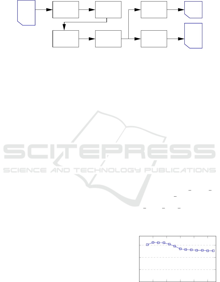
Figure 1: Processing pipeline of the segmentation method.

To this end, we utilised octree subsampling and time

rescaling, modiﬁcations to the clustering algorithms,

and a special post-processing for dealing with under-

segmentation that is inherent to the clustering algo-

rithms. After mapping the subsampled clusters back

to the original data, the ﬂight trajectories can be inter-

polated with a LOWESS (Cleveland, 1979) multivari-

ate regression based on the time as a single predictor.

All of these methods are described in section 2.

We evaluated our method on a series of DVS

recordings provided by the BeeVision project, where

insect events had already been segmented from other

events with a lightweight U-Net (Pohle-Fr

ohlich

et al., 2024). This enabled us to evaluate the algo-

rithm both with and without the presence of back-

ground noise stemming from shaking leaves, varying

illumination due to clouds, or other random effects.

The evaluation is described in section 3.

2 SEGMENTATION METHOD

The segmentation algorithm takes an unlabelled point

cloud with time and space coordinates as input and

returns two output lists: For each point, a cluster label

or a noise label is computed, and for every non-noise

cluster a ﬁtted ﬂight path is computed and sampled

at equidistant timestamps. The processing pipeline

of the algorithm is shown in Figure 1. It consists of

the following steps: Pre-processing, clustering, post-

processing, ﬁtting of ﬂight paths using the LOWESS

method, and remapping the labels to the original point

cloud. Additionally, after reading of the input CSV-

ﬁle, the timestamp is scaled by a scaling factor that

was determined for representative data.

During pre-processing, the data is subsampled and

outliers are removed. This smaller point cloud is then

clustered. The clustering has a tendency to underseg-

ment nearby insect tracks. These tracks are therefore

corrected in the post-processing step. Afterwards,

curves representing ﬂight paths are ﬁtted and the spa-

tial curve position is computed for equidistant times-

tamps. Since the clustering was done on only the

subsampled and ﬁltered data, labels must be prop-

agated to the points that were removed during pre-

processing. To this end, every unlabelled point re-

ceives the label of the nearest labelled point. The in-

dividual steps are described in detail in the following

subsections.

2.1 Pre-Processing

The timestamp dimension t is of a different unit (mi-

croseconds) and thus differs several orders of mag-

nitude from the spatial dimensions (pixel). With the

original timescale of microseconds, the distances in

the temporal dimension thus dominate the distances

of the spatial dimensions, which has a serious nega-

tive impact on the performance of DBSCAN and the

MST-based clustering methods.

We therefore scale the time with a data based scal-

ing factor. As the DVS recording scenario is the same

for all recorded data, it was sufﬁcient to estimate an

appropriate scaling factor only once from a represen-

tative subset of the data. We have chosen the scaling

factor s such that the mean distances to the k-th near-

est neighbour in the spatial direction d

(k) and d

(k)

is equal to the mean distance d

(k) in the t direction,

i.e.

s · d

(k) =



(k) + d

(k)



/2 (1)

It is interesting to note that the scale factor s was quite

robust with respect to the choice of k, as can be seen

·10

−4

scale factor s

Figure 2: Dependency of the scaling factor s according to

Eq. (1) on the number of neighbours k.

VISAPP 2025 - 20th International Conference on Computer Vision Theory and Applications

Figure 3: Subsampling: grey points are the original point

cloud and the red crosses are the subsampled points.

in Figure 2. Moreover, we have observed that either

choice in this range resulted in a similar performance

of the clustering algorithm, and we have settled on

s = 5.3 · 10

−4

µs

−1

After scaling the timestamps, an octree-based sub-

sampling is applied in order to reduce both data

volume and noise. Octree subsampling works by

constructing a tree structure that recursively divides

the 3D space into eight evenly-sized cubes, stop-

ping at a predeﬁned depth (Meagher, 1982). This

process leaves the non-empty space divided into

cubes, and for each cube a representative point is se-

lected. These representative points form the subsam-

pled point cloud. To make the ﬁltering effect inde-

pendent from the size of the point cloud, we chose the

side length of the cube at the lowest level of the octree

as the stopping criterion instead of the depth. A larger

value causes more ﬁltering and a smaller value less ﬁl-

tering. In our use case, the full octree data structure

was not needed, because no nearest-neighbour queries

are done on the full point cloud, only on the subsam-

pled data. We therefore divide the space directly into

cubes.

There are different options to select the represen-

tative point, e.g., the point closest to the centroid of

the cube, or the point closest to the centroid of the

points in the cube. This, however, has only little ef-

fect on the results. A result of the subsampling step

is shown in Figure 3. The octree subsampling has the

positive side-effect that it can also be used for remov-

ing noise in sparse regions simply by skipping cubes

with fewer points than a deﬁned threshold. This sim-

ple noise reduction step does not increase the run-

time; it only requires some additional space since the

skipped points have to be memorised in order to ob-

tain the noise label in the remapping step.

2.2 Clustering

As neither the number of insect tracks, nor their shape

is known, we cannot use clustering algorithms like

k-means that look for spherical clusters and a given

number of clusters. A characteristic of insect ﬂight

trajectories is that they typically are represented by re-

gions with a higher point density and are separated by

less dense regions. It is thus natural to use a clustering

points

edges

inconsistentedges

Figure 4: The MST of two clusters with an “inconsistent

edge” highlighted in green and the points coloured by clus-

ter.

method based on closeness of points and thus a local

density. We have implemented both DBSCAN and

MST-based clustering as alternative options. Both are

clustering algorithms that can detect clusters of arbi-

trary shape and do not require the number of clusters

beforehand.

MST-based clustering algorithms build a weighted

graph with weights corresponding to the Euclidean

distance between node points, and remove “inconsis-

tent edges” from the Minimum Spanning Tree (MST)

of this graph (Zahn, 1971). Edges are considered “in-

consistent” if they have a weight that is above some

global or local distance threshold. This splits the MST

into connected components which represent the clus-

ters. The MST-based clustering method is illustrated

in Figure 4 with the MST of two insect tracks. The

inconsistent edge highlighted in green is removed,

which results in two connected components repre-

senting insect tracks. These can be easily identiﬁed

using graph traversal techniques such as breadth-ﬁrst

or depth-ﬁrst search.

In general, building an MST for N nodes has run-

time complexity O(N

), but as our distance is Eu-

clidean, it is not necessary to build the complete

distance matrix and the runtime can be reduced to

O(N log N) (March et al., 2010). Moreover, we could

rely on a fast Open Source C++ implementation by

Andrii Borziak

Due to a considerable spread in point density be-

tween different tracks, local thresholds for identifying

inconsistent edges resulted in undersegmentation. We

therefore used a global threshold for removing incon-

sistent edges, which was chosen in dependence of the

length d of the pre-processing octree cube diagonal as

5 · d. However this threshold is chosen, there are two

unavoidable problems: Splits due to gaps in partially

occluded tracks, and merges of tracks coming close to

https://github.com/AndrewB330/EuclideanMST

Separation of Insect Trajectories in Dynamic Vision Sensor Data

Figure 5: MST-based segmentation works in the example

on the left, and fails in the example on the right. The same

occurs for DBSCAN.

each other. An example can be seen in Figure 5.

The MST-based clustering also offers a simple

method identify falsely recognised clusters in dense

regions that actually represent noise. When the edges

are traversed in the MST, the mean edge weight can

be calculated. Clusters with a small mean edge weight

can be removed as they often consist of noise. This

method adds more robustness against very strong

noise, which is common in DVS-recordings and can-

not be removed by the ﬁltering in the subsampling

step.

DBSCAN (Ester et al., 1996) is a density-based

clustering algorithm, that deﬁnes clusters as regions

of high density that are separated by regions of lower

density. DBSCAN has two parameters, eps and

minPts. Every point with at least minPts neighbours

within a radius of eps is a core point. Whenever an

unlabelled core point is found, a new cluster is ini-

tialised and the core point is added to it. The new

cluster is iteratively propagated to core points within

radius eps. This process is iterated until all core points

and their neighbours are assigned to clusters. Points

that are not neighbours of a core point are marked as

outliers.

Schubert et al. (Schubert et al., 2017) suggested

simple heuristics for choosing the parameters. For

minPts, they suggested minPts = 2· #Dimensions = 6,

which we have adopted. We have not utilised their

suggestion to analyse a ’k-dist plot’ to determine an

appropriate eps, because the octree cell size of our

subsampling process already limits the possible max-

imum point density. We therefore set eps equal to a

multiple of the diagonal of the cube, which is the fur-

thest distance between two points in a dense insect

track should be separated. After experimentally test-

ing different values for the multiplication factor, we

settled on eps = 6 · d, where d is the diagonal length

of a cell in the pre-processing octree.

Like MST-based clustering, DBSCAN cannot

separate tracks when insect tracks come close to each

(a) After clustering.

(b) After post-processing.

Figure 6: Example for two merged tracks that are correctly

split up during post-processing.

other (see Figure 5), because both algorithms are

purely based on point distances. To correct this prob-

lem, a post-processing step is necessary.

2.3 Post-Processing

To separate touching insect tracks that were erro-

neously merged into the same cluster, we imple-

mented a post-processing that consists of three steps.

First, possibly merged clusters are identiﬁed and, sec-

ondly, these clusters are split up at branching points

in their Minimum Spanning Tree (MST). As the split-

ting leads to oversegmentation, that is corrected in the

third step by merging the most appropriate branches

based on their direction and time alignment. An ex-

ample can be seen in Figure 6.

2.3.1 Identifying Merged Clusters

To minimise runtime and prevent over-segmentation,

we ﬁrst detect merged clusters using a simple heuris-

tic. This approach is based on the premise that when

insect tracks intersect, there should be simultaneous

activity in different spatial regions at the same time.

As an indicator for this phenomenon, we compute the

spatial Euclidean distance between consecutive time

points for each cluster, which results in an array of

n − 1-values which we call ∆s. The computation is

facilitated by the nature of the DVS stream, which

records events according to their time order, so that

consecutive points occur at similar times.

If the standard deviation of the array sd(∆s) ex-

ceeds a threshold θ

, the cluster is ﬂagged for further

VISAPP 2025 - 20th International Conference on Computer Vision Theory and Applications

curve0

curve1

curve2

Figure 7: Example for oversegmentation due to splitting at

crossing points.

post-processing steps. In the longest recording and

for the threshold value θ

= 22.36 that worked best

in our case, 16 out of 598 clusters met this criterion,

including all 12 merged tracks and 4 incorrect classi-

ﬁcations.

2.3.2 Splitting Clusters

For each ﬂagged cluster, an MST is built and nodes

with three or more branches of sufﬁcient depth are

identiﬁed as split points. The depth threshold is cho-

sen proportional (α · n

) in order to adapt it to varying

cluster sizes.

At each split point, all edges except the short-

est one are deleted. This splits the cluster into con-

nected components, which are identiﬁed and num-

bered. These preliminary clusters are referred to as

segments. These must be further processed, though,

because the splitting method can result in overseg-

mentation at X-crossing points where the straight con-

tinuation cannot be preserved (see Figure 7).

2.3.3 Merging Over-Segmented Components

To correct over-segmentation due to MST splitting,

segments are merged again, if they are continuations

of each other in the direction extrapolated from the

end of the earlier segment. For every segment S

that occurred during splitting the clusters at branches,

another ﬁtting segment S

is sought as continuation.

Both the time order of both segments is considered,

as well as the direction of the segments around the

ends with the closest timestamps.

Only segments S

with timestamps greater than S

within a given tolerance and with a sufﬁciently small

gap, are considered. The time difference between the

last point of S

) and the ﬁrst point of S

) must

satisfy:

−0.5 · θ

tolerance

< t

− t

< θ

t tolerance

(2)

This allows for gaps of the length θ

t tolerance

and an

Figure 8: Curves ⃗x(t) ﬁtted with LOWESS for two insect

tracks. The ﬁtted curves are coloured and the DVS points

are shown in grey.

overlap of half of θ

t tolerance

. The gap length has to

be greater than the tolerance of overlap because one

insect often covers the other. This leads to large gaps

in the track. A time overlap that large, however, did

not occur in our data, which is why 0.5 was somewhat

arbitrarily chosen to reduce the allowed overlap. A

threshold that worked in our case was, in the original

time unit, θ

t tolerance

= 35ms.

For approximating the outgoing and incoming di-

rection, ⃗v

and ⃗v

out

of the tracks, the ﬁrst PCA com-

ponent of the beginning and end of every segment is

calculated. The size of the beginning and end is de-

termined by a proportion of the size of the segment.

The similarity of the directions is measured with

the cosine similarity, and a segment S

is only consid-

ered as a continuation of segment S

, if

cos(⃗v

,⃗v

out

) > θ

mincos

= 0.7 (3)

Moreover, there is the constraint that each segment

cannot be used more than once as a continuation of

another segment. If more than one segment fulﬁls all

conditions, the segment with the maximal cosine sim-

ilarity cos(⃗v

,⃗v

out

) is chosen as the continuation.

2.4 Curve Fitting

For visualisation or for an analysis of insect ﬂight

patterns, it is useful to represent each track as a spa-

tial curve ⃗x(t) that yields a position for every time t.

As each point in our point cloud already has a time

stamp, this time coordinate can be used as a predic-

tor in a local regression model with the space coor-

dinates as a multivariate response variable. An es-

tablished method for local regression is Cleveland’s

Locally Weighted Estimated Scatterplot Smoothing

(LOWESS) (Cleveland, 1979). We used the Open

Source C++ implementation CppWeightedLowess

Aaron Lun.

https://github.com/LTLA/CppWeightedLowess

Separation of Insect Trajectories in Dynamic Vision Sensor Data

Figure 9: Example result showing the clustering of the points into noise (red) and different insect tracks (other colours).

For each time value t, LOWESS ﬁts a second or-

der polynomial locally through the r neighbouring

points in the predictor space, which is the time in our

case. Apart from only using the nearest neighbours,

the points are also inversely weighted according to

their distance in the predictor space. This restricts the

regression further to the local shape. From a set of

sample points, LOWESS predicts a response ⃗x(t) for

arbitrary predictor values t within the sample range,

but the resulting curve is non-parametric. We there-

fore compute the predicted x and y coordinates for

equally spaced timestamps and store both together as

the result of the curve ﬁtting.

The result of LOWESS depends on the number

of neighbours that are used for local ﬁtting, which

is determined by a parameter f , also known as span.

A smaller value for f produces a less smooth curve,

whereas a larger value result in a smoother curve. f

can be given as a proportion of the entire set, e.g.

10%, or as a ﬁxed number of neighbours. A curve

tangential to the ﬂight direction is only obtained, if

the neighbourhood extends much more in the ﬂight

direction than perpendicular to it. Unfortunately, this

means that a ﬁxed number of neighbours does not

work for ﬁtting insect tracks in general, because in-

sects vary considerable in size and wing beat rate,

which means that the number of DVS events per time

interval can vary considerably. Therefore, we chose

0.2 as value for f , i.e. 20% of the points per cluster

were used to ﬁt each value. As can be seen in Figure

8. This may result in overly smoothed curves, how-

ever, in cases of very long clusters.

3 RESULTS

We have evaluated our algorithm on eight recordings

of insect ﬂights on a meadow that were captured in the

context of the BeeVision project (Pohle-Fr

ohlich and

Bolten, 2023). The data was recorded with a Proph-

esee EVK3 Gen4.1 event camera (1280 × 720 resolu-

tion), where time was recorded in microseconds. The

length varied between 16 and 160 seconds, compris-

ing 308MB and about 10

events. The data points had

already been segmented with a U-Net (Pohle-Fr

ohlich

et al., 2024), and the time was scaled to milliseconds.

To obtain ground truth data, the ﬁles were man-

ually labelled, assigning each insect track a unique

label and an additional label for points considered to

be noise. This was done with the Semantic Segmenta-

tion Editor

that allows for 3D point cloud labelling.

To assess the ground truth labelling, a sample of the

test data was labelled manually again a few months

apart from the ﬁrst pass. This provided a reference

value for the accuracy of the labelling.

To evaluate the post-processing, 19 merges of sev-

eral tracks into one cluster were identiﬁed in the

dataset and isolated with some surrounding clusters.

To assess the robustness of our algorithm with respect

to noise, both the original dataset with noise and the

dataset without noise were used.

3.1 Evaluation Criteria

There are two categories of evaluation criteria for the

evaluation of clusterings, internal and external in-

dices (Hassan et al., 2024). Internal indices, like the

Silhouette Index and Calinski-Harabasz Index, assess

clusters based on properties such as intra- and inter-

cluster variance, but they assume clusters are spheri-

cal and are thus not suitable for insect tracks.

External metrics compare the clustering results

with ground truth data. These metrics evaluate clus-

terings by counting whether pairs of points fall in the

https://github.com/Hitachi-Automotive-And-Industr

y-Lab/semantic-segmentation-editor

VISAPP 2025 - 20th International Conference on Computer Vision Theory and Applications

Figure 10: Example for the result of noise removal: red points are noise, the time is on the x-axis and the y-axis is the y-

coordinate.

same or different clusters in the respective cluster-

ings. From these counts, the (adjusted) Rand Index

and the Jaccard Score are computed (Hubert and Ara-

bie, 1985). The Rand Index measures overall similar-

ity, ranging from 0 (no matching pairs) to 1 (identical

clusterings), while the adjusted Rand Index corrects

for chance. The Jaccard Score is similar but only

focuses on pairs that are in the same cluster in both

ground truth and predicted clustering. This has the

effect that the Jaccard Score is always smaller than

the Rand Index.

Since these metrics are pair-based, larger clusters

(or tracks) with more point pairs will have a greater

impact on the evaluation results. Moreover, although

their range is [0,1], it is not clear which values actu-

ally represent “good” results. We therefore compared

the two manual ground truth clusterings of the same

data set and obtained a Jaccard-Score of about 0.86

and an adjusted Rand-Score of 0.92. This means that

results around these values can be considered as good

results for our algorithm.

3.2 Clustering

As can be seen from the results in Table 1, in the ab-

sence of noise, the MST-based clustering and DB-

SCAN both have an excellent performance that is

comparable to a human. In the presence of noise,

however, DBSCAN performs considerably poorer.

This is because the MST-based clustering removes

more less dense clusters than DBSCAN. An exam-

ple of its ability to remove noise is seen in Figure 10,

where the insect track is mostly separated from the

noise with only some small artefacts.

According to Table 1, it seems that the post-

processing has almost no effect on the quality of

the segmentation. This is misleading, however, be-

cause the pairwise quality indices are dominated by

the large clusters and not very sensitive to differences

in small clusters. Therefore, we did another test with

only those clusters that were erroneously merged by

Table 1: Jaccard score J and adjusted Rand index R

ad j

for

the two clustering algorithms with and without noise or with

and without post-processing.

post- MST DBSCAN

noise proc. R

ad j

J R

ad j

no no 0.921 0.857 0.919 0.854

no yes 0.922 0.858 0.922 0.858

yes no 0.759 0.656 0.598 0.470

yes yes 0.765 0.662 0.589 0.467

the clustering algorithms. Out of 19 merged cluster,

the post-processing split 11 correctly, and 3 were cor-

rectly split, but not perfectly rejoined. The same test

for non-merged clusters yielded no incorrect splits.

Noise removal worked best with uniformly dis-

tributed noise but had problems when noise is con-

centrated in speciﬁc areas, e.g., due to ambient ef-

fects like wind. For the full original noisy record-

ing with points removed only when are the only point

in an octree cube or when they end up in a cluster

of only one point, 70.8% of all noise points are cor-

rectly removed, while 1.3% of insect points were in-

correctly removed. This criterion is thus too strict for

raw noisy data. Weaker thresholds are required for

noisy datasets, although more aggressive ﬁltering dis-

proportionally affects small insect tracks. More ﬁlter-

ing will also remove points at the edges of the insect

tracks, which could impact the insect classiﬁcation

downstream. With simulated uniformly distributed

noise consisting of about 197% of the original point

cloud size, 99.98% of noise points are removed, while

only 5.78% of insect points are affected.

3.3 Runtime

When the method is utilised for actual real-life in-

sect monitoring, it is crucial that the processing oc-

curs in real time, i.e., the runtime must be less than

the recording time of the DVS sensor plus other pre-

processing time possibly needed, e.g. for computing

3D spatial information from stereo recordings (Pohle-

ohlich et al., 2024). Figure 11 shows how the aver-

Separation of Insect Trajectories in Dynamic Vision Sensor Data

0 100 200 300

Duration of the DVS−recording [s]

Runtime [s]

group

Writing

Reading

Pre−processing

Remapping

Clustering

LOWESS

Post−processing

Figure 11: The runtime plotted against the length of the

DVS-recording and separated into the individual steps of

the processing pipeline.

age runtime varies with the DVS-recording duration

and how it is distributed among the different process-

ing steps. The runtime was measured on an AMD

Ryzen 7 5700U CPU running Ubuntu 20.04 and aver-

aged over 100 runs. As can be seen from Figure 11,

the processing runtime is always considerably shorter

than the duration of the recording.

We also measured the speedup S due to pre-

processing, deﬁned as the runtime without subsam-

pling divided by the runtime with subsampling. The

speedup for noise ﬁltering was greater in unnoisy data

(S ≈ 20) than in noisy data (S ≈ 4). This is because

subsampling reduces the number of noisy points less

effectively, as many noise points occupy their own

cubes. The speedup for noisy data increases with

noise removal during subsampling. This in partic-

ular affected the MST-based clustering which had a

speedup of 30. This means that subsampling is essen-

tial for an application in real time.

4 CONCLUSIONS

We have developed a method for fast instance seg-

mentation of insect ﬂight tracks in DVS data, treating

time as another dimension to preserve high temporal

resolution. The central part of the algorithm is a den-

sity based clustering, for which either DBSCAN or

MST-based clustering can be chosen. The MST-based

clustering was considerably more robust with respect

to noise and is thus preferable. Both algorithms, how-

ever, failed to separate close by tracks, and we have

implemented a post-processing step that remedies this

shortcoming in most situations.

Due to subsampling during pre-processing, the

method has a runtime much shorter than the DVS

recording duration and is thus applicable in real time.

Noise removal was optionally included in the subsam-

pling step and in the clustering step. These automatic

noise detection makes the method quite robust in the

presence of noise, which is important for its deploy-

ment in natural scenarios.

Although the method has an accuracy comparable

to a manual segmentation by a human, it occasionally

removes thin tracks. This makes the method currently

less effective for small insects like mosquitos. For

visualisation or further analysis, we also ﬁt ﬂight tra-

jectories through the returned clusters. Although our

usage of LOWESS was satisfactory, a local regres-

sion based on the number of neighbours can become

problematic for scenarios with a wide range of track

thicknesses and lengths. It would be interesting to in-

vestigate different local regression methods, e.g. by

basing the local region on ﬁxed time intervals.

Although we tested our method only with DVS

data with two spatial dimensions, there is nothing spe-

cial in our algorithm that restricts it to 2D data. The

method can thus readily be deployed to 3D data like

that recorded by the new system developed in the Bee-

Vision project (Pohle-Fr

ohlich et al., 2024), which

aims at counting insect populations over a long pe-

riod. We plan to deploy our algorithm in this project

and use it as a second step after semantic segmenta-

tion. This will then be followed by a classiﬁcation

step which leads to an automatic counting of species

occurances in the data.

REFERENCES

Cleveland, W. S. (1979). Robust locally weighted regres-

sion and smoothing scatterplots. Journal of the Amer-

ican Statistical Association, 74(368):829–836.

Dalitz, C., Ayyad, Y., Wilberg, J., Aymans, L., Bazin, D.,

and Mittig, W. (2019a). Automatic trajectory recog-

nition in Active Target Time Projection Chambers

data by means of hierarchical clustering. Computer

Physics Communications, 235:159–168.

Dalitz, C., Wilberg, J., and Aymans, L. (2019b). TriplClust:

An algorithm for curve detection in 3D point clouds.

Image Processing On Line, 8:26–46.

Ester, M., Kriegel, H.-P., Sander, J., Xu, X., et al. (1996).

A density-based algorithm for discovering clusters in

large spatial databases with noise. In kdd, volume 96,

pages 226–231.

Hallmann, C. A., Sorg, M., Jongejans, E., Siepel, H.,

Hoﬂand, N., Schwan, H., Stenmans, W., M

uller,

A., Sumser, H., H

orren, T., et al. (2017). More

VISAPP 2025 - 20th International Conference on Computer Vision Theory and Applications

than 75 percent decline over 27 years in total ﬂy-

ing insect biomass in protected areas. PloS one,

12(10):e0185809.

Hassan, B. A., Tayfor, N. B., Hassan, A. A., Ahmed, A. M.,

Rashid, T. A., and Abdalla, N. N. (2024). From A-to-Z

review of clustering validation indices. Neurocomput-

ing, 601:128198.

Hubert, L. and Arabie, P. (1985). Comparing partitions.

Journal of classiﬁcation, 2:193–218.

March, W. B., Ram, P., and Gray, A. G. (2010). Fast Eu-

clidean minimum spanning tree: algorithm, analysis,

and applications. In Proceedings of the 16th ACM

SIGKDD international conference on Knowledge dis-

covery and data mining, pages 603–612.

Meagher, D. (1982). Geometric modeling using octree en-

coding. Computer graphics and image processing,

19(2):129–147.

Pohle-Fr

ohlich, R. and Bolten, T. (2023). Concept study for

dynamic vision sensor based insect monitoring. In In-

ternational Conference for Computer Vision and Ap-

plications (VISAPP), pages 411–418.

Pohle-Fr

ohlich, R., Gebler, C., and Bolten, T. (2024).

Stereo-event-camera-technique for insect monitoring.

In International Conference for Computer Vision and

Applications (VISAPP), pages 375–384.

Rovere, M., Chen, Z., Di Pilato, A., Pantaleo, F., and Seez,

C. (2020). CLUE: A fast parallel clustering algo-

rithm for high granularity calorimeters in high-energy

physics. Frontiers in Big Data, 3:591315.

Schubert, E., Sander, J., Ester, M., Kriegel, H. P., and Xu, X.

(2017). DBSCAN revisited, revisited: why and how

you should (still) use DBSCAN. ACM Transactions

on Database Systems (TODS), 42(3):1–21.

Zahn, C. T. (1971). Graph-theoretical methods for detecting

and describing gestalt clusters. IEEE Transactions on

Computers, 100(1):68–86.

Separation of Insect Trajectories in Dynamic Vision Sensor Data