Uncertainty-Driven Past-Sample Selection for Replay-Based Continual

Learning

Anxo-Lois Pereira

3 a

, Eduardo Aguilar

1,2 b

and Petia Radeva

1 c

Dept. de Matem

atiques i Inform

atica, Universitat de Barcelona, Gran Via de les Corts Catalanes 585, Barcelona, Spain

Dept. de Ingenier

ıa de Sistemas y Computaci

on, Universidad Cat

olica del Norte, Angamos 0610, Antofagasta, Chile

Dept. d’Enginyeria Inform

atica i Matem

atiques, Universitat Rovira i Virgili, Avda. Pa

ısos Catalans 26, Tarragona, Spain

Keywords:

Continual Learning, Replay, Rehearsal, Uncertainty Quantiﬁcation, Evidential Deep Learning.

Abstract:

In a continual learning environment, methods must cope with catastrophic forgetting, i.e. avoid forgetting

previously acquired knowledge when new data arrives. Replay-based methods have proven effective for this

problem; in particular, simple strategies such as random selection have provided very competitive results. In

this paper, we go a step further and propose a novel approach to image recognition utilizing a replay-based

continual learning method with uncertainty-driven past-sample selection. Our method aims to address the

challenges of data variability and evolving databases by selectively retaining and revisiting samples based on

their uncertainty score. It ensures robust performance and adaptability, improving image classiﬁcation accu-

racy over time. Based on uncertainty quantiﬁcation, three groups of methods were proposed and validated,

which we call: sample sorting, sample clustering, and sample ﬁltering. We experimented and evaluated the

proposed methods on three public datasets: CIFAR10, CIFAR100 and FOOD101. We obtained very encour-

aging results largely outperforming the baseline sample selection method for rehearsal on all the datasets.

1 INTRODUCTION

Continual Learning (CL), or lifelong learning, gathers

together work and approaches that tackle the problem

of learning when the data distribution changes over

time, and where knowledge fusion over never-ending

streams of data needs to be accounted for (Lesort

et al., 2020). Traditional Machine Learning models

typically require retraining from scratch with the en-

tire dataset whenever new data is introduced, which is

both time-consuming and computationally expensive.

In contrast, CL aims to enable the model to learn con-

tinuously from new data streams, making the process

more efﬁcient and scalable. However, CL is explicitly

limited by catastrophic forgetting (Wang et al., 2024),

which refers to the sudden and severe loss of prior

information in learning systems when acquiring new

information (Jedlicka et al., 2022).

To avoid catastrophic forgetting, strategies based

on regularization, architecture, and rehearsal have

been proposed (Masana et al., 2023). Speciﬁcally, in

https://orcid.org/0009-0004-9766-1418

https://orcid.org/0000-0002-2463-0301

https://orcid.org/0000-0003-0047-5172

the rehearsal-based method, a subset of the data used

for training is retained to preserve prior knowledge

in a CL framework. Several approaches have been

proposed for exemplar selection, such as: random-

based methods (Guo et al., 2022; Prabhu et al., 2020),

distance-based methods (Rebufﬁ et al., 2017), error-

based methods (Toneva et al., 2018), methods based

on parameter updating (Aljundi et al., 2019b; Aljundi

et al., 2019a; Sun et al., 2022), and those used for the

selection of CoreSet (Yoon et al., 2022; Hao et al.,

2023). Despite attempts to improve the sample se-

lection, the simplest method Random Selection (Guo

et al., 2022), continues to be the one commonly cho-

sen in CL and ends up being one of the best for the

rehearsal (Brignac et al., 2023; Borsos et al., 2020;

Yoon et al., 2022; Guo et al., 2022).

On the other hand, uncertainty-based approaches

have proven very effective in improving the under-

standing of the deep learning models (Abdar et al.,

2021). In particular, by analyzing epistemic uncer-

tainty it is possible to categorize the complexity of

the data as a function of the features learned dur-

ing training (Nagarajan et al., 2023). Data with high

epistemic uncertainty means being underrepresented

(e.g., a hard sample (Nagarajan et al., 2023) or OoD

Pereira, A.-L., Aguilar, E. and Radeva, P.

Uncertainty-Driven Past-Sample Selection for Replay-Based Continual Learning.

DOI: 10.5220/0013140700003912

Paper published under CC license (CC BY-NC-ND 4.0)

In Proceedings of the 20th International Joint Conference on Computer Vision, Imaging and Computer Graphics Theory and Applications (VISIGRAPP 2025) - Volume 3: VISAPP, pages

365-372

ISBN: 978-989-758-728-3; ISSN: 2184-4321

365

data (Aguilar et al., 2023)). On the other hand, data

with low epistemic uncertainty corresponds to data

well-represented (e.g. an easy sample) in the training

dataset. We hypothesize that the uncertainty score re-

lated to each sample may be a good indicator when se-

lecting a suitable example to retain prior knowledge.

There are various approaches to quantify uncer-

tainty (Abdar et al., 2021), among which Evidential

Deep Learning (EDL) (Sensoy et al., 2018) stands out

for its ease of implementation and ability to quantify

uncertainty efﬁciently in terms of computational re-

sources. By integrating EDL into a CL framework, it

is possible to give conﬁdence in a prediction given a

particular sample after each class-incremental learn-

ing step, and thus identify and prioritize past samples

that are most likely to improve model performance

and robustness.

To address the challenge of catastrophic forget-

ting, this paper proposes an innovative replay-based

CL method that uses uncertainty-based selection of

past samples. Our approach, which takes advan-

tage of quantiﬁed uncertainty through an EDL-based

method, not only improves the model’s ability to re-

tain previously learned information, but also ensures

that new knowledge is integrated more effectively.

The main contributions of this paper are as fol-

lows: 1) We are the ﬁrst to use EDL uncertainty quan-

tiﬁcation within the CL paradigm in a sample selec-

tion scheme for rehearsal; 2) We designed several

sample selection approaches based on uncertainty; 3)

We evaluated our sample selection approaches in 3

public benchmarking datasets: CIFAR10, CIFAR100,

and FOOD101; and 4) We outperformed the baseline

sample selection strategy with an improvement of up

to 2.21%, 3.05% and 4.13% in terms of AccFinal,

Acc1st, and Forgetting, respectively.

The rest of the paper is organized as follows: Sec-

tion 2 describes the proposed EDL-based Rehearsal

methods. In Section 3, the dataset, experimental se-

tups, and validation metrics are detailed. Section 4

shows the results of the proposed methods and base-

line for multiplies incremental settings. Finally, Sec-

tion 5 concludes the works and presents the future di-

rections.

2 METHODOLOGY

CL claims to create models that are able to adapt

to new situations and domains. Under CL, the Ma-

chine Learning method is trained iteratively as new

classes or new data arrive or are added to the model.

When the method is trained only with the new data,

it can completely forget the previous data, which is

called catastrophic forgetting. To avoid this, rehearsal

is used, where a small sample of previously learned

data is employed to avoid forgetting it. Considering a

Class-incremental learning scenario, we hypothesize

that uncertainty can provide us with a good perspec-

tive for selecting samples that preserve knowledge of

the seen classes.

In the following subsection, we ﬁrst detail the

EDL-based method and then our proposed rehearsal

methods based on the uncertainty quantiﬁed after

each incremental step (also called experience).

2.1 Evidential Deep Learning

Uncertainty in deep learning can be interpreted as

how conﬁdent the model is in the prediction it has

made about a sample. In the sample selection litera-

ture, there are many interpretations and implementa-

tions of uncertainty for training deep learning mod-

els, such as the use of Kullback-Leibler divergence

in CAL or other CoreSet (Guo et al., 2022) methods

such as Least Conﬁdence, Entropy and Margin (Cole-

man et al., 2020).

Unlike the previous methods, in this study, we

follow the implementation of the uncertainty mea-

sure presented in (Sensoy et al., 2018; Aguilar et al.,

2023), which is based on Evidence Theory, as this

method considers the performance achieved in object

recognition, the quality of the estimated uncertainty,

and the computational resources required. To un-

derstand how this method of quantifying uncertainty

works, we must ﬁrst deﬁne how the evidence e is cal-

culated:

= σ( f

)); α

= e

+ 1. (1)

where e

is the evidence of a sample x

function f

(·)

returns the output logits, or prediction, of a sample

using a neural network with the θ weights. It is im-

portant to note that this neural network does not have

a softmax layer or another activation layer at the end,

which makes the result of applying f

) on a sample

return the output logits of the sample x

prediction

and not the conﬁdences of the predictions. To calcu-

late the evidence, a non-linearity must be applied to

ensure that the evidence is non-negative. This func-

tion is the function σ(·). Several functions can be

used to fulﬁll the role of the σ(·) function. For exam-

ple, in the original implementation, the authors used

the ReLU function (Sensoy et al., 2018). However, in

this study, we ended up using the exponential func-

tion exp(·), which is non-linear and ensures that the

result is greater than 0, considered to be more stable

than the ReLU (Bao et al., 2021; Aguilar et al., 2023).

On the other hand, we have the deﬁnition of α in the

VISAPP 2025 - 20th International Conference on Computer Vision Theory and Applications

366

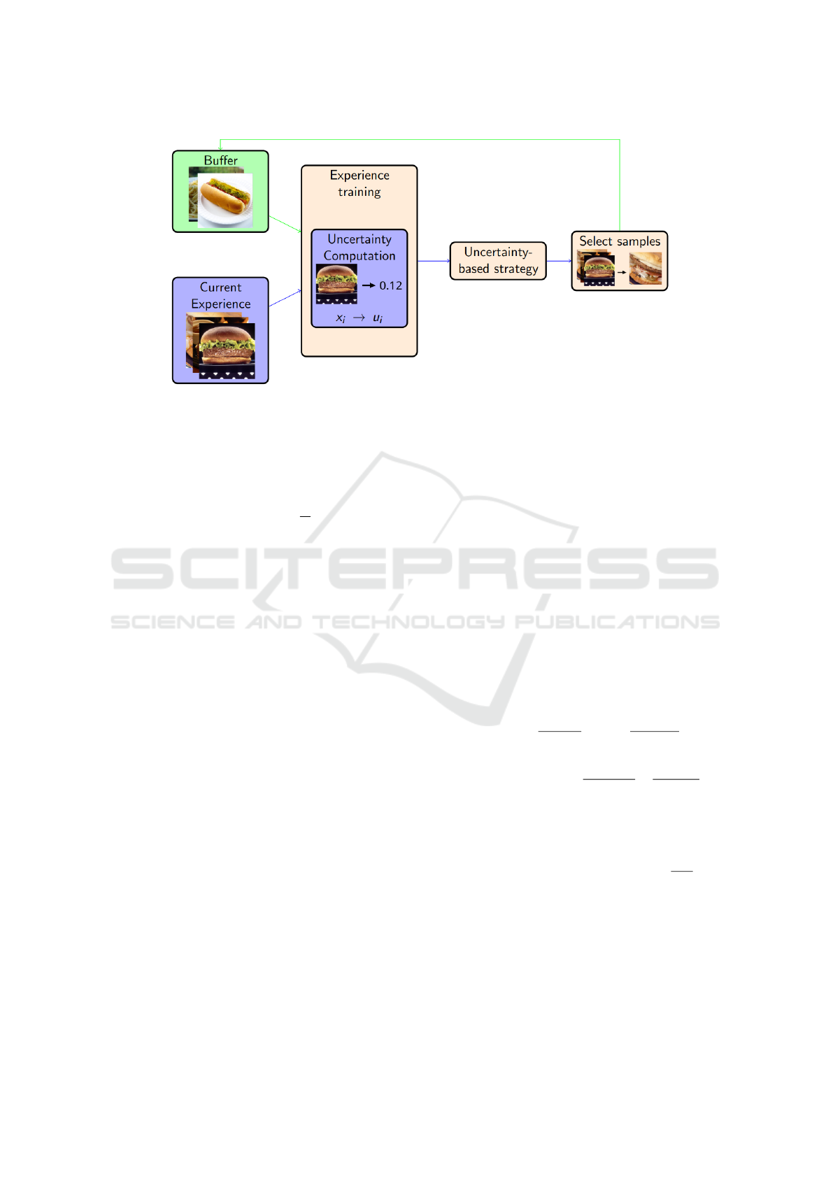
Figure 1: Illustrative diagram of uncertainty calculation and sample selection.

equation (1), which represents the parameters of the

Dirichlet distribution, being greater than or equal to

1. Taking into account that K is the number of classes

in the experiment, the uncertainty is calculated as fol-

lows:

∑

j=1

i j

; u

(2)

where α

i j

is the value of α given for the j-th class of

the i-th sample. With this and taking into account that

i j

∈ [1, inf), S

∈ [K, inf) is ensured. Thus, u

∈ (0, 1]

where the value of maximum uncertainty i.e. 1 is only

taken, if the value of α, and therefore the evidence is

minimum (α

i j

= 1, ∀ j). With this deﬁnition, an un-

certainty value can be assigned to each of the training

samples, at the moment of training the model with

those samples, to obtain a value that can be sorted for

each of them, so that it can be used to select samples

for the rehearsal.

For the uncertainty to be properly calculated and

used for sample selection in rehearsal, the logits re-

sulting from the model must have values that allow

the correct interpretation of the evidence. For this, it

is necessary to change the training loss from Cross-

Entropy to the one used for Evidential Deep Learning

(Sensoy et al., 2018; Aguilar et al., 2023). Originally,

the use given to the deﬁnition of uncertainty used in

this study was to check how conﬁdent the model was

about the predictions of a given sample on a classical

Deep Learning framework. To give a correct predic-

tion of this value, the designers of this method, devel-

oped a loss function based on this implementation of

uncertainty to train the models. This loss function is

based on the Evidential Deep Learning (Sensoy et al.,

2018) method, or EDL for short, and is the Type II

Maximum Likelihood. For simplicity, we will refer to

this loss as EDL in the remainder of this study.

Given the sample x

and its ground-truth y

in a

one-hot vector encoding, the EDL loss function is cal-

culated as such that:

i j

(

1, if k = j

0, otherwise

(3)

∑

j=1

i j

× (log(S

) − log(α

i j

)) (4)

The value L

is the principal term of the loss of the

sample x

. An extra term is considered to act as a reg-

ularization to avoid providing evidence on misclassi-

ﬁed samples. This is carried out by the KL-divergence

and is calculated as follows:

i j

= e

i j

× (1 − y

i j

) + 1; S

∑

j=1

i j

(5)

= ln

Γ(S

)

Γ(K)

−

∑

j=1

Γ(α

i j

)

Γ(1)

(6)

∑

j=1

(α

i j

−1) × (

′

(α

i j

)

Γ(α

i j

)

−

′

)

Γ(S

)

) (7)

= KL

+ KL

. (8)

In these equations, lnΓ(·) is the natural logarithm

of the absolute value of the gamma function Γ(·), such

that lnΓ(·) = ln|Γ(·)|. At the same time,

′

(x)

Γ(x)

is the

logarithmic derivative of the Γ function.

Finally, the EDL loss function is deﬁned as:

EDL

= (1 − λ) × L

+ λ × (C

ann

× KL

). (9)

where λ is equal to 0.1 and C

ann

is an annealing co-

efﬁcient, which can be deﬁned as a constant value or

as a value that mutates as training progresses. In this

study, C

ann

is equal to 0.01 throughout the training.

Uncertainty-Driven Past-Sample Selection for Replay-Based Continual Learning

367

2.2 EDL-Based Rehearsal Methods

Uncertainty is used as a measure of conﬁdence for

each sample during inference, calculated after each

experience in the proposed methods’ training. Based

on the uncertainty of predictions for each sample, we

propose several strategies to select samples that retain

more information, helping to prevent catastrophic for-

getting. These strategies range from simple to com-

plex. A diagram illustrating the training process us-

ing any of these uncertainty-based sample selection

strategies is provided in Figure 1.

The simplest strategy is based on Samples Sort-

ing. Speciﬁcally, the proposed strategy named Simple

Uncertainty involves sorting the samples according to

their uncertainty and selecting those with the lowest

uncertainty. By doing so, the model will be trained

in future experiences with the samples that the model

can classify more reliably.

Another approach, based on Sample Clustering,

aims to ensure that the selected samples are as evenly

distributed as possible in terms of uncertainty. To

achieve this, we propose clustering the samples using

the K-Means algorithm. From each cluster, we se-

lect an equal number of samples, if possible, to main-

tain an even distribution. The samples can then be

chosen in various ways, such as randomly, which we

call Kmeans Random, or by iteratively selecting the

most central sample, i.e., the one closest to the me-

dian, which we call Kmeans Median.

The last approach, based on Samples Filtering,

considers eliminating the samples with the highest un-

certainty and then applying another strategy to ensure

that the chosen samples do not stray too far from what

the model has been able to learn. Two strategies have

been considered. First, by choosing the samples at

random over the non-eliminated samples, which we

call Filtered Random. Secondly, by eliminating the

samples and then applying the technique of Kmeans

Random, which we call Filtered Kmeans.

3 EXPERIMENTS

In this section, we explain the datasets used and jus-

tify their use. Then, we describe the hyperparameters

used in the training and their value. Finally, we deﬁne

the evaluation metrics used to compare the results.

3.1 Datasets

The study utilized three datasets, each serving a dif-

ferent purpose. CIFAR10 (Krizhevsky et al., 2009)

was used for preliminary validation of the proposed

methods on a small, simple dataset. CIFAR100

(Krizhevsky et al., 2009), an extension of CIFAR10

with more classes, was used to assess how the meth-

ods perform with a more complex dataset. The third

dataset, Food101 (Bossard et al., 2014), was used to

evaluate the methods in a much more complex do-

main, featuring large image sizes, several classes, and

high intra-class variability and inter-class similarity.

CIFAR10: consists of 10 classes, with 6,000 im-

ages per class—5,000 for training and 1,000 for eval-

uation, totaling 50,000 training and 10,000 evalua-

tion images. Its simplicity, due to the small number

of classes (10) and small image size (32x32 RGB),

makes it ideal for fast training and testing in a contin-

ual learning (CL) paradigm.

CIFAR100: is an extension of CIFAR10, featur-

ing 100 classes instead of 10, with the same num-

ber of images. Each class contains 600 RGB im-

ages—500 for training and 100 for evaluation—at the

same 32x32 size. While it shares the advantages of

CIFAR10, such as small image size for fast training

and widespread use as a benchmark, the increased

number of classes and reduced images per class make

training more challenging.

Food101: contains 101 food classes, with 750 train-

ing images and 250 evaluation images per class, total-

ing 101,000 images. It is still widely used while not a

standard benchmark like the other datasets. Due to its

larger size and increased complexity compared to CI-

FAR10 and CIFAR100, it is more challenging to train

on.

3.2 Experimental Setup

In all experiments for all datasets and models equiv-

alently, we deﬁned the same type of buffer and pre-

pared the CL framework. Following the experimental

setup used in Deepcore (Guo et al., 2022), we used

a variable memory size buffer, where in a balanced

way (per experience), we kept a small percentage of

the samples for rehearsal. Speciﬁcally, we decided to

keep 10% of the samples of each experience in the

buffer. We focus on this range of percentage of sam-

ples because, for this range in (Guo et al., 2022) the

authors observed that the baseline random selection

results are notably higher compared to those of more

complex strategies.

The model trained in these experiments is the

ResNet-18 (He et al., 2016). These networks usu-

ally give outstanding results regardless of the train-

ing dataset, which has led to a standard benchmark-

ing model within an image classiﬁcation problem.

Speciﬁcally, ResNet-18 is widely used in the litera-

ture to compare benchmarking (Masana et al., 2023;

VISAPP 2025 - 20th International Conference on Computer Vision Theory and Applications

368

Aguilar et al., 2023). For these reasons, we have de-

cided to use it within our study as the model to train

and evaluate our sample selection strategies for re-

hearsal.

To simulate a real-world scenario within a CL ex-

perimental setting, a Class-incremental learning sce-

nario was employed. The target dataset is divided into

several class groups, which are trained iteratively, one

after the other. These training phases, involving sub-

sets of classes, are referred to as experiences. It is evi-

dent that if the classes are entirely isolated, the classes

from the ﬁrst experience may be completely forgotten

by the last one, a phenomenon known as catastrophic

forgetting.

The main hyper-parameters for training and re-

hearsal depended largely on the dataset, but remained

stable throughout all experiments done with each

dataset. The Table 1 lists these main parameters.

In this table, the columns Epochs and Increments,

given the training dataset, show the number of train-

ing epochs done in each experience and the number

of classes that are trained in each experience (without

counting the data in the rehearsal buffer) respectively.

The Base column is the number of classes that are

trained in the ﬁrst experience of a given dataset. As

for the number of training experiences, we set it at a

total of 5. It is important to note that these parameters

do not fully apply to the robustness and generalization

experiments. For these experiments, we have tested

multiple combinations of the number of training ex-

periences and the percentage of the samples that are

stored in the memory buffer.

Table 1: Hyper-parameters used in the training of experi-

ments per dataset.

Dataset Epochs Increments Base

CIFAR10 10 2 2

CIFAR100 50 20 20

FOOD101 120 20 21

Other hyper-parameters had to be deﬁned to con-

duct the benchmarking experiments. These hyper-

parameters were evaluated in the CIFAR10 dataset

and then used for the three datasets. The ﬁrst hyper-

parameter was the number of clusters for the Kmeans-

based methods, where 15 was found to be the best

number consistently, except for the Filtered Kmeans

method, where 50 was found to be slightly better

sometimes. In the Filtered methods, we found that

the best percentage of data to remove before apply-

ing the selection algorithm is 20%. These values

were found experimentally in the CIFAR10 dataset

and used for all the datasets. The only exception to

this is the Learning Rate used. Both CIFAR datasets

were trained in the benchmarking experiments using

0.005 as the learning rate, while for FOOD101 0.001

was used instead.

All the models (all the experiments for all the

methods) were trained using as initial weights the

pre-trained on ImageNet (Krizhevsky et al., 2012)

ResNet-18. Also, to be able to correctly train these

datasets in the ResNet-18 neural network, some pre-

processing of the images and some data augmenta-

tion had to be applied. For the FOOD101 dataset,

a random ﬂip is applied for data augmentation rea-

sons. Then the image is resized to 256 × 256 and ran-

domly cropped into a size of 224 × 224, which is the

pre-trained ResNet-18 input size. Finally, the image

is normalized. Similarly, the CIFAR datasets are ﬁrst

cropped into 32×32 using padding = 4 as a data aug-

mentation technique (note that the original size was

already 32 × 32). Then the image is randomly ﬂipped

horizontally and resized into 224 × 224. Finally, they

are normalized taking into account the mean and stan-

dard deviation of ImageNet.

3.3 Validation Metrics

To evaluate and compare the sample selection meth-

ods for rehearsal, we have mainly used accuracy,

which computation follows the equation (10), where

T P = True positive, FP = False positive, T N = True

negative and FN = False negative; the mean accuracy

(Acc) on the test set. Formally, the Acc in a CL prob-

lem can be deﬁned as follows:

Acc

T P

+ T N

T P

+ T N

+ FP

+ FN

(10)

where Acc

denotes the average accuracy calculated

after the j-th experience of the data corresponding to

the new classes incorporated in the i-th experience.

There are two accuracy-based metrics selected

to evaluate model performance called AccFinal and

Acc1st which are deﬁned as follows:

AccFinal = Acc

1,...,nE

; Acc1st = Acc

. (11)

As can be seen in the equation (11), the ﬁnal aver-

age accuracy, AccFinal, calculates the accuracy after

the last experience considering data from all classes.

On the other hand, the metric Acc1st represents the

average accuracy of the data belonging to the classes

of the data used in the ﬁrst experience, computed after

the whole training process is completed.

In addition to the accuracy, the Forgetting met-

ric was used. This metric is calculated as the mean

over the difference between the accuracy obtained af-

ter the ﬁrst training on the data corresponding to the

new classes used in an experience and the accuracy

Uncertainty-Driven Past-Sample Selection for Replay-Based Continual Learning

369

obtained on the same experience data after the last ex-

perience, as in the equation (12), where Acc

is the

accuracy of the experience i after the whole training

ﬁnished (after last experience training) and Acc

is the

accuracy of the experience i after the training of the

said experience i has ﬁnished. Unlike accuracy, the

less the Forgetting value is, the better the result is:

Forgetting =

∑

i=1

Acc

− Acc

. (12)

4 RESULTS

This section presents a comparative analysis of the

proposed sample selection strategies, followed by a

comparison of the best strategy with the baseline. Fi-

nally, it includes an evaluation of the robustness and

generalizability of both strategies.

4.1 Evaluation of the Proposed Scores

for Sample Selection

Using the parameters stipulated in Table 1, we trained

on the CIFAR10 dataset with ﬁve different seeds for

each strategy. The results of the strategies on the

test set are summarized in Table 2. As can be seen,

the strategies belonging to Sample Filtering are the

ones that provide the best performance. In contrast,

the performance of the Simple Uncertainty strategy

differs greatly from the rest. The best performance

is achieved with Filtered Kmean, which provides a

noticeable improvement over the second best strat-

egy (Filtered Random) of 0.75%, 2.82% and 1.23%

in terms of AccFinal, Acc1st and Forgetting.

However, it should be noted that CIFAR10 has a

small number of classes, and the results may not nec-

essarily be the same in other scenarios involving more

classes. Therefore, we evaluated the same experi-

ments on a similar domain, but with 10 times more

classes, which is CIFAR100. As this dataset is more

complicated than CIFAR10, more training epochs are

needed. The results are shown in the Table 2. In the

CIFAR100 case, the strategy with the best average re-

sults in terms of AccFinal was the Simple Uncertainty

strategy. This method is closely followed for all the

Sample Filtering methods. On the other hand, for the

other metrics, the Filtered Random strategy gives con-

sistently better results, outperforming the rest of the

strategies.

Finally, we evaluated the most promising meth-

ods on the FOOD101 dataset. It should be noted that,

due to the very slow training with this dataset, only

four methods have been trained with only three seeds,

compared to the ﬁve seeds used for the other two

datasets. The results can be found in Table 2 for all

the metrics. Both strategies Simple Uncertainty and

Filtered Random provide comparable results in terms

of AccFinal. For the other metrics, Filtered Random

got the best results and was closely followed by Sim-

ple Uncertainty for the Acc1st and Filtered Kmeans

Random for the Forgetting.

Taking into account the performance obtained

among all the datasets, the strategy Filtered random

is selected for comparison with the baseline approach

because, although it is not always the best, it is the

strategy that provides the most stable behavior.

4.2 Comparison with Baseline

Approach

Table 3 shows the results obtained by the baseline

approach and the Filtered Random on the CIFAR10,

CIFAR100 and Food101 datasets. Overall, the pro-

posed strategy outperforms the baseline in all met-

rics evaluated, i.e., in terms of AccFinal, Acc1st

and Forgetting. The improvement is most notice-

able in the more challenging datasets (CIFAR100

and FOOD101). Particularly, in FOOD101, an im-

provement of the 2.21%, 3.07% and 2.12% in terms

of AccFinal, Acc1st and Forgetting. These re-

sults demonstrate the importance of using uncertainty

quantiﬁcation to ﬁlter out samples with a high degree

of uncertainty before proceeding to random selection,

in order to obtain a better subset that will help pre-

serve prior knowledge and thus mitigate catastrophic

losses. On the other hand, it is interesting to note that

several of the proposed uncertainty-based strategies

other than Filtered Random, for some datasets, per-

form better, as seen in Table 2, and thus the results

difference is even greater.

4.3 Robustness and Generalizability

Analysis

The performance analysis is extended by consider-

ing different numbers of experiences and buffer sizes.

This allows us to evaluate the ability of the proposed

strategy to mitigate catastrophic forgetting in different

Class-incremental learning scenarios. The results are

presented in Table 4 for the baseline and the proposed

strategy for the CIFAR100 dataset. As expected, the

greater the number of experiences or the smaller the

buffer size, the greater the forgetting. A great im-

provement of the proposed strategy is seen in all con-

ﬁgurations except for 20 experiences and a buffer size

of 0.2. This demonstrates the generalizability of the

VISAPP 2025 - 20th International Conference on Computer Vision Theory and Applications

370

Table 2: Performance of the proposed strategies on the CIFAR10, CIFAR100 and FOOD101 datasets.

Dataset Strategy AccFinal ↑ Acc1st ↑ Forgetting ↓

CIFAR10 Kmean Random (k=15) 0.8934 ± 0.0096 0.8437 ± 0.0598 0.0454

Kmean Median (k=15) 0.8945 ± 0.0069 0.8526 ± 0.0619 0.0437

Filtered Random 0.8975 ± 0.0113 0.8653 ± 0.0842 0.0531

Filtered Kmean (k=15) 0.9050 ± 0.0122 0.8935 ± 0.0545 0.0408

Filtered Kmean (k=50) 0.9010 ± 0.0143 0.8789 ± 0.0481 0.0485

Simple Uncertainty 0.8624 ± 0.0233 0.8209 ± 0.0911 0.1170

CIFAR100 Kmeans Random (k=15) 0.5250 ± 0.0283 0.4499 ± 0.0266 0.3312

Kmeans Median (k=15) 0.4958 ± 0.0332 0.4209 ± 0.0506 0.3630

Filtered Random 0.5670 ± 0.0127 0.5241 ± 0.0374 0.2739

Filtered Kmeans (k=15) 0.5513 ± 0.0110 0.4994 ± 0.0426 0.2980

Filtered Kmeans (k=50) 0.5684 ± 0.0184 0.5155 ± 0.0585 0.2792

Simple Uncertainty 0.5689 ± 0.0276 0.4940 ± 0.0455 0.2943

FOOD101 Filtered Random 0.5076 ± 0.0164 0.4795 ± 0.0407 0.2898

Filtered Kmeans (k=15) 0.4789 ± 0.0209 0.4422 ± 0.0123 0.3215

Simple Uncertainty 0.5084 ± 0.0146 0.4677 ± 0.0393 0.3271

Table 3: Comparison of the selected best strategy with the baseline on the CIFAR10, CIFAR100 and FOOD101 datasets.

Dataset Strategy AccFinal ↑ Acc1st ↑ Forgetting ↓

CIFAR10 Random EDL 0.8927 ± 0.0275 0.8575 ± 0.0910 0.0571

Filtered Random 0.8975 ± 0.0113 0.8653 ± 0.0842 0.0531

CIFAR100 Random EDL 0.5544 ± 0.0112 0.4824 ± 0.0491 0.2856

Filtered Random 0.5670 ± 0.0127 0.5241 ± 0.0374 0.2739

FOOD101 Random EDL 0.4855 ± 0.0353 0.4491 ± 0.0261 0.3311

Filtered Random 0.5076 ± 0.0164 0.4795 ± 0.0407 0.2898

Table 4: Performance in terms of Forgetting for several incremental settings and buffer sizes on CIFAR100 dataset.

Buffer size : 0.1 0.05 0.2

Strategy Experiences Forgetting ↓ Forgetting ↓ Forgetting ↓

Random EDL 20 0.3556 0.4366 0.2973

Filtered Random 20 0.3392 0.4198 0.3168

Random EDL 10 0.3161 0.3873 0.2628

Filtered Random 10 0.2993 0.3775 0.2176

Random EDL 5 0.2856 0.3515 0.2393

Filtered Random 5 0.2739 0.3281 0.2355

proposed strategy for other buffer sizes and its robust-

ness to retain knowledge when performing more ex-

periences.

5 CONCLUSIONS

In this paper, we proposed several uncertainty-based

sample selection method strategies and evaluated

them on three public datasets. From the results,

we observe in the CIFAR10 and CIFAR100 datasets,

that at least one of the proposed strategies surpasses

the Random selection baseline in all validation met-

rics. Similarly, in FOOD101 dataset, all evaluated

uncertainty-based sample selection strategies, except

Filtered Kmeans, outperform the baseline. Among

all the datasets, the most consistent method is Fil-

tered Random. Particularly, in the large datasets (CI-

FAR100 and FOOD101), we found that although in

terms of AccFinal the strategy Simple Uncertainty it

is better (and much worse in the CIFAR10 dataset) by

a small margin, in the two other evaluation metrics

(Acc1st and Forgetting) Filtered Random is consis-

tently better. The experimental results demonstrate

that the predictive uncertainty related to each sample

provides relevant information for sample selection.

Speciﬁcally, the proposed best strategy can be inter-

preted as improving Random selection by ﬁltering

high-uncertainty data before selection. With this ﬁl-

tering was possible to improve the mitigation of catas-

trophic forgetting. In future work, we will explore the

integration of uncertainty into other strategies used in

Uncertainty-Driven Past-Sample Selection for Replay-Based Continual Learning

371

replay-based methods to analyze whether uncertainty

provides complementary information to improve the

sample selection they perform.

ACKNOWLEDGEMENTS

This work has been partially supported by the Span-

ish project PID2022-136436NB-I00 (AEI-MICINN),

Horizon EU project MUSAE (No. 01070421),

2021-SGR-01094 (AGAUR), Icrea Academia’2022

(Generalitat de Catalunya), Robo STEAM (2022-

1-BG01-KA220-VET-000089434, Erasmus+ EU),

DeepSense (ACE053/22/000029, ACCI

O), Deep-

FoodVol (AEI-MICINN, PDC2022-133642-I00),

PID2022-141566NB-I00 (AEI-MICINN), Beatriu de

os Programme and the Ministry of Research and

Universities of the Government of Catalonia (2022

BP 00257), and Agencia Nacional de Investigaci

on y

Desarrollo de Chile (ANID) (Grant No. FONDECYT

INICIACI

ON 11230262).

REFERENCES

Abdar, M., Pourpanah, F., Hussain, S., Rezazadegan, D.,

Liu, L., Ghavamzadeh, M., Fieguth, P., Cao, X., Khos-

ravi, A., Acharya, U. R., et al. (2021). A review

of uncertainty quantiﬁcation in deep learning: Tech-

niques, applications and challenges. Information fu-

sion, 76:243–297.

Aguilar, E., Raducanu, B., Radeva, P., and Van de Weijer,

J. (2023). Continual evidential deep learning for out-

of-distribution detection. In ICCV Workshop, pages

3444–3454.

Aljundi, R., Belilovsky, E., Tuytelaars, T., Charlin, L., Cac-

cia, M., Lin, M., and Page-Caccia, L. (2019a). Online

continual learning with maximal interfered retrieval.

In NeurIPS, pages 11849–11860.

Aljundi, R., Lin, M., Goujaud, B., and Bengio, Y. (2019b).

Gradient based sample selection for online continual

learning. In NeurIPS, pages 11816–11825.

Bao, W., Yu, Q., and Kong, Y. (2021). Evidential deep

learning for open set action recognition. In ICCV,

pages 13349–13358.

Borsos, Z., Mutny, M., and Krause, A. (2020). Coresets via

bilevel optimization for continual learning and stream-

ing. In NeurIPS.

Bossard, L., Guillaumin, M., and Van Gool, L. (2014).

Food-101–mining discriminative components with

random forests. In ECCV, pages 446–461. Springer.

Brignac, D., Lobo, N., and Mahalanobis, A. (2023). Im-

proving replay sample selection and storage for less

forgetting in continual learning. In ICCV, pages 3540–

3549.

Coleman, C., Yeh, C., Mussmann, S., Mirzasoleiman, B.,

Bailis, P., Liang, P., Leskovec, J., and Zaharia, M.

(2020). Selection via proxy: Efﬁcient data selection

for deep learning. In ICLR.

Guo, C., Zhao, B., and Bai, Y. (2022). Deepcore: A compre-

hensive library for coreset selection in deep learning.

In International Conference on Database and Expert

Systems Applications, pages 181–195. Springer.

Hao, J., Ji, K., and Liu, M. (2023). Bilevel coreset selection

in continual learning: A new formulation and algo-

rithm. In NeurIPS.

He, K., Zhang, X., Ren, S., and Sun, J. (2016). Deep resid-

ual learning for image recognition. In CVPR, pages

770–778.

Jedlicka, P., Tomko, M., Robins, A., and Abraham, W. C.

(2022). Contributions by metaplasticity to solving

the catastrophic forgetting problem. Trends in Neu-

rosciences, 45(9):656–666.

Krizhevsky, A., Hinton, G., et al. (2009). Learning multiple

layers of features from tiny images.

Krizhevsky, A., Sutskever, I., and Hinton, G. E. (2012). Im-

agenet classiﬁcation with deep convolutional neural

networks. In NeurIPS, pages 1106–1114.

Lesort, T., Lomonaco, V., Stoian, A., Maltoni, D., Fil-

liat, D., and D

ıaz-Rodr

ıguez, N. (2020). Continual

learning for robotics: Deﬁnition, framework, learning

strategies, opportunities and challenges. Information

fusion, 58:52–68.

Masana, M., Liu, X., Twardowski, B., Menta, M.,

Bagdanov, A. D., and van de Weijer, J. (2023).

Class-incremental learning: Survey and performance

evaluation on image classiﬁcation. IEEE TPAMI,

45(5):5513–5533.

Nagarajan, B., Bola

nos, M., Aguilar, E., and Radeva, P.

(2023). Deep ensemble-based hard sample mining for

food recognition. Journal of Visual Communication

and Image Representation, 95:103905.

Prabhu, A., Torr, P. H. S., and Dokania, P. K. (2020).

Gdumb: A simple approach that questions our

progress in continual learning. In ECCV, volume

12347 of Lecture Notes in Computer Science, pages

524–540. Springer.

Rebufﬁ, S., Kolesnikov, A., Sperl, G., and Lampert, C. H.

(2017). icarl: Incremental classiﬁer and represen-

tation learning. In CVPR, pages 5533–5542. IEEE

Computer Society.

Sensoy, M., Kaplan, L., and Kandemir, M. (2018). Evi-

dential deep learning to quantify classiﬁcation uncer-

tainty. NeurIPS, 31.

Sun, Q., Lyu, F., Shang, F., Feng, W., and Wan, L. (2022).

Exploring example inﬂuence in continual learning.

NeurIPS, 35:27075–27086.

Toneva, M., Sordoni, A., des Combes, R. T., Trischler, A.,

Bengio, Y., and Gordon, G. J. (2018). An empirical

study of example forgetting during deep neural net-

work learning. In ICLR.

Wang, L., Zhang, X., Su, H., and Zhu, J. (2024). A compre-

hensive survey of continual learning: theory, method

and application. IEEE TPAMI.

Yoon, J., Madaan, D., Yang, E., and Hwang, S. J. (2022).

Online coreset selection for rehearsal-based continual

learning. In ICLR.

VISAPP 2025 - 20th International Conference on Computer Vision Theory and Applications

372