Learning-Based Reconstruction of Under-Sampled MRI Data Using
End-to-End Deep Learning in Comparison to CS
Adnan Khalid
1
, Husnain Shahid
2
, Hatem A. Rashwan
1
and Domenec Puig
1
1
Departament d’Enginyeria Inform
`
atica i Matem
`
atiques, Universitat Rovira i Virgili, Tarragona, Spain
2
Centre Tecnol
`
ogic de Telecomunicacions de Catalunya (CTTC), Barcelona, Spain
Keywords:
Image Reconstruction, Compressed Sensing, Under-Sampled Measurements, Deep Learning.
Abstract:
Magnetic Resonance Imaging (MRI) reconstruction, particularly restoration and denoising, remains challeng-
ing due to its ill-posed nature and high computational demands. In response to this, Compressed Sensing (CS)
has recently gained prominence for enabling image reconstruction from limited measurements and conse-
quently reducing computational costs. However, CS often struggles to maintain diagnostic image quality and
strictly relies on sparsity and incoherence conditions that are somewhat challenging to meet with experimental
data or particularly real-world medical data. To address these limitations, this paper proposes a novel frame-
work that integrates CS with a convolutional neural network (CNN), effectively relaxing the CS constraints
and enhancing the diagnostic quality of MRI reconstructions. In essence, this method applies CS to gener-
ate a measurement vector during initial step and then refined the output by CNN to improve image quality.
Extensive evaluations on the MRI knee dataset demonstrate the efficacy of this dual step approach, achieving
significant quality improvements with measurements (SSIM = 0.876, PSNR = 27.56 dB). A deep comparative
analysis also perform to identify the superior performance over multiple existing CNN architectures.
1 INTRODUCTION
Magnetic Resonance Imaging (MRI) has gained sig-
nificant attention in medical imaging due to its excep-
tional ability to produce high-resolution images sur-
passing other modalities like CT scans and X-rays.
Nevertheless, despite being a highly effective diag-
nostic tool, MRI frequently has a significant limita-
tion: its lengthy acquisition time. This means that pa-
tients often have to lie still for long periods during the
scan, which can be uncomfortable and inconvenient.
As a result, one of the primary goals in MRI research
has been finding ways to shorten these scan times.
To this end, an important technique known as
Parallel Imaging (PI) has been introduced (Griswold
et al., 2005). This method leverages multiple coils to
capture different views of the body simultaneously,
which are then combined through software to cre-
ate the final image. PI techniques are generally di-
vided into two main categories: those that operate in
the imaging domain and those that work with k-space
data (Ying et al., 2006). Using k-space data more ef-
ficiently and applying the Fourier Transform (FT) to
make it sparse helps accelerate the imaging process,
but it also introduces under-sampling artifacts that can
degrade image quality (Brau et al., 2008).
To accelerate MRI further, researchers have turned
to CS (Sartoretti et al., 2019). By acquiring only a
subset of the data needed for a full scan, CS-based
techniques can reconstruct images faster and at a
lower computational cost. Combined with PI, this
approach offers a promising way to produce high-
resolution MRI images more quickly. However, re-
constructing high-quality images from this limited
data remains a challenging and hence an active area
of research.
Although CS-based approaches have indeed made
progress in speeding up MRI reconstruction (Lustig
et al., 2008) (Feng et al., 2017), they often come with
their own set of problems. On one hand, these meth-
ods can reduce the time it takes to reconstruct an im-
age, but with the cost of compromising the diagnostic
quality and relying on complex, iterative algorithms
that are computationally demanding. In some cases,
it may take more time to reconstruct just one image,
which makes real-time MRI reconstruction imprac-
tical. Moreover, CS-based techniques depend heav-
ily on certain mathematical conditions, like sparsity
and incoherence (Provost and Lesage, 2008), which
are not always easy to meet with real-world data
Khalid, A., Shahid, H., Rashwan, H. A. and Puig, D.
Learning-Based Reconstruction of Under-Sampled MRI Data Using End-to-End Deep Learning in Comparison to CS.
DOI: 10.5220/0013141400003912
Paper published under CC license (CC BY-NC-ND 4.0)
In Proceedings of the 20th International Joint Conference on Computer Vision, Imaging and Computer Graphics Theory and Applications (VISIGRAPP 2025) - Volume 3: VISAPP, pages
373-380
ISBN: 978-989-758-728-3; ISSN: 2184-4321
Proceedings Copyright © 2025 by SCITEPRESS – Science and Technology Publications, Lda.
373

with various orthogonal features. For instance, dif-
ferent types of images require different sparse repre-
sentations: smooth images are typically sparse in the
Fourier domain, while images with sharp edges might
be better represented in wavelet or curvelet domains
(Lustig et al., 2007). This variability makes it diffi-
cult to find the perfect sparse basis, limiting the effec-
tiveness of CS-based methods, especially when data
from different modalities are integrated to generalize
the performance of the method.
To overcome these limitations, researchers have
increasingly turned to deep learning, which has rev-
olutionized many fields, including medical imaging.
Deep learning, especially convolutional neural net-
works (CNNs), has shown impressive results in tasks
like image classification (Wang et al., 2020), segmen-
tation (Ronneberger et al., 2015), and reconstruction
(Zhang and Dong, 2020). In the context of medi-
cal imaging, CNNs have been used to enhance the
quality of MRI and CT scans (Chen et al., 2017)
(Jin et al., 2017)(Wang et al., 2016), offering a more
adaptive and data-driven approach to image recon-
struction. These models typically require structured
CS data as input to produce the best results (Can-
des, 2008). When dealing with high-resolution MRI
images, the network complexity can become over-
whelming, which is why it’s often necessary to break
the data into smaller slices or transform it into a sparse
domain before feeding it into the network (He et al.,
2016a). In addition to these limitations, such ap-
proaches necessitate training the network and adjust-
ing parameters for each specific sampling ratio, as
they typically rely on a fixed measurement matrix.
To cope with these issues, this paper takes advan-
tage of an integrated approach that combines a non-
iterative CS technique (designed without enforcing
sparsity to speed up recovery) with a deep learning-
based method to ensure the results meet diagnostic-
quality standards. In CS component, this method uses
a specified subset of measurements to reconstruct the
image, which then serves as the input to the deep
learning framework without the need for image slic-
ing, thus accelerating the overall process. Essentially,
fewer measurements lead to faster MRI reconstruc-
tion. To tackle the under-sampling artifacts that result
from using a limited number of measurements, the
proposed framework employ a Deep Learning-based
Convolutional Neural Network (CNN). As direct ac-
cess to k-space data is often unavailable from the hos-
pitals due to privacy concerns, we simulate under-
sampled measurements from dense images, which are
then used as inputs to the deep learning network for
validation, which is a true depiction of using real work
data, which could be present in any unknown domain.
Additionally, by utilizing a random measurement ma-
trix, the proposed approach enables training the net-
work just once for all possible sampling ratios rather
than requiring re-training for each different under-
sampling ratio.
The structure of this paper is as follows: Section 2
discusses the typical CS technique in the reconstruc-
tion domain, the proposed framework, and a variety
of deep learning networks to be compared to identify
the better network. Section 3 details the experimental
materials, while Section 4 presents the results and dis-
cussions. Finally, Section 5 concludes the paper with
a summary of key findings.
2 METHODS
This paper defines a supervised learning method to
help with the problems caused by sparsity-based ap-
proaches. This method makes it possible to recon-
struct MRI images from data that is not well-sampled
without using sparsity constraints.
As illustrated in Fig. 1, a compressed sensing-
based approach is first applied to the input data in
R
N×N
. The image data is then transformed into a R
M
measurement vector by multiplying with a random
measurement matrix, where M ≪ N. The measure-
ment vector is subsequently processed by a fully con-
nected layer to produce a preliminary image proxy.
Figure 1: Measurement images are generated using this pro-
cedure for various undersampling ratios.
The resulting image may initially display artifacts
and blurring. A deep learning based approach is then
utilized to correct the undersampling artifacts, gener-
ating a high-resolution reconstruction of the image.
2.1 Compressed Sensing for Image
Reconstruction
In CS theory, data consisting of N samples can be
mapped into a sparse representation by applying an
appropriate sparse transform Ψ, defined as:
θ = Ψx
In CS, the sparse representation of the original im-
age x is denoted by θ, where x comprises N pixels.
Sparsity is defined by the condition ∥θ∥
ℓ
0
≪ N, with
VISAPP 2025 - 20th International Conference on Computer Vision Theory and Applications
374

the ℓ
0
-norm representing the number of non-zero el-
ements in θ. The primary objective of CS is to ac-
curately reconstruct the image x from a reduced set of
measurements acquired by the imaging system. Given
that the measurement vector y is obtained via a sens-
ing matrix L, the relation between the measurements
and the original image can be expressed as:
y = Lx
In this context, reconstructing the k-space image can
be formulated as the following convex optimization
problem (Wang et al., 2017),
min∥θ∥
ℓ
0
s.t. y = LΨ
−1
θ
In this framework,Ψ represents the sparse transform,
while L corresponds to the measurement matrix. For
CS to be effective, the matrix product LΨ must ex-
hibit the necessary properties of a valid CS matrix.
Minimizing the ℓ
0
-norm, which measures the number
of non-zero entries in the sparse representation, typ-
ically leads to a combinatorial optimization problem,
rendering it computationally impractical for high-
resolution image reconstruction. To address this, it
has been established that minimizing the ℓ
1
yields
equivalent results in most cases, provided the solu-
tion is sufficiently sparse. The resulting optimization
problem is justified as follows:
min∥θ∥
ℓ
1
s.t. y = LΨ
−1
θ
In practical scenarios, MRI data often do not exhibit
perfect sparsity on a predetermined transform basis,
which poses a significant challenge for CS methods
to achieve accurate image reconstruction (Provost and
Lesage, 2008). A key limitation of CS is its depen-
dency on a reduced number of measurements, even
when an optimal sparse basis Ψ is identified. Addi-
tionally, as previously discussed, the matrix product
LΨ must satisfy the essential requirements of a CS
matrix. Specifically, this matrix must exhibit suffi-
cient linear independence across small subsets of its
columns or satisfy the restricted isometry property
(RIP) to enable efficient and accurate recovery of the
data. As outlined by (Candes, 2008), the RIP condi-
tion is defined as:
(1 − δ
s
)∥θ∥
2
2
≤ ∥Aθ∥
2
2
≤ (1 + δ
s
)∥θ∥
2
2
where 0 < δ
s
< 1 is the restricted isometry con-
stant, and A = LΨ is the sensing matrix. For sparse
vectors θ, RIP ensures that any two different sparse
vectors can be distinguished from their measurement
vectors. Specifically, if two measurement vectors
y
1
= Ax
1
and y
2
= Ax
2
cannot be distinguished, ac-
curate reconstruction of the sparse vectors becomes
impossible. Therefore, ensuring that the sensing ma-
trix A satisfies the RIP is critical for successful recon-
struction. However, in practice, MRI data typically
do not conform to the perfect sparsity on a fixed ba-
sis (Bastounis and Hansen, 2017), leading to failure
to meet the RIP condition and consequently limiting
the effectiveness of reconstruction.
2.2 Deep Learning Approach
CNN’s network architecture is highly important in
solving different reconstruction problems. However,
choosing an optimal CNN architecture for a given
dataset and task is not straightforward. We compared
different CNN architectures for MRI reconstructions
and quantitatively analyzed their performances indi-
vidually. The core objective in this framework is
to develop a mapping function ξ : R
M×M
→ R
N×N
.
The design of such a mapping function assumes the
availability of a paired dataset, where each pair con-
sists of a corrupted image V
n
and its corresponding
artifact-free ground truth Y
n
, forming a training set
T = {(V
n
,Y
n
)}
N
n=1
. Leveraging deep learning prin-
ciples, the nonlinear mapping function ξ is learned
through an optimization process to minimize the dis-
crepancy between the network output and the ground
truth. Specifically, the performance of the mapping
function ξ is quantified by the total training error, ex-
pressed as (Mousavi and Baraniuk, 2017):
E(T ; ξ) =
N
∑
n=1
e(ξ(X
n
),Y
n
)
Here, e : R
N×N
×R
N×N
→ R represents the loss func-
tion, which computes the error between the predicted
image ξ(X
n
) and the true image Y
n
during the training
process. The ultimate aim is to optimize ξ such that
it accurately maps the input measurements to artifact-
free, high-quality reconstructions. The various Deep
Learning (DL) networks utilized in this study are de-
scribed as follows:
2.2.1 SegNet
The SegNet architecture (Badrinarayanan et al., 2017)
is designed for pixel-wise semantic segmentation
based on deep Fully Convolutional Neural Networks.
The convolution layers with filter banks followed by
batch normalization are applied to produce the set
of feature maps in the encoder network. Afterward,
element-wise rectified linear (ReLU) non-linearity is
formulated as g(x) = max(0.0, x). To achieve trans-
lation invariance in feature maps, max pooling with
a (2, 2) window and stride of 2 across many layers is
implemented. On the other hand, the decoder network
is set to upsample its input feature maps from corre-
sponding encoder feature maps. Besides, to perform
non-linear reconstruction of the input image size, the
Learning-Based Reconstruction of Under-Sampled MRI Data Using End-to-End Deep Learning in Comparison to CS
375

upsampling is performed based on the indices used
in the max-pooling operation of the encoder network.
SegNet is proved efficient in terms of both memory
and computation time.
2.2.2 UNet
The UNet (Ronneberger et al., 2015) was originally
proposed for medical image segmentation and can be
trained end-to-end using a small number of samples.
It has also shown promising results in photoacous-
tic microscopy (PAM) and photoacoustic tomogra-
phy (PAT) image reconstruction and denoising (Guan
et al., 2019). The UNet architecture can be viewed
as a two-stage network. The first stage consists of
a series of encoding layers that increase the number
of features while reducing the spatial dimensions of
the input image. In the decoding part of the UNet,
the latent space features from the encoding part are
concatenated with up-sampled layers at each decoder
stage to construct the output image. Additionally, the
skip concatenation connections within the architec-
ture allow the decoder to learn features that may be
lost during the max-pooling operations in the encoder.
Figure 2: The contraction and expansion part of UNet archi-
tecture consists of Convolutional operations, max-pooling
layers, ReLU activation function, Concatenation, and Up-
sampling layers.
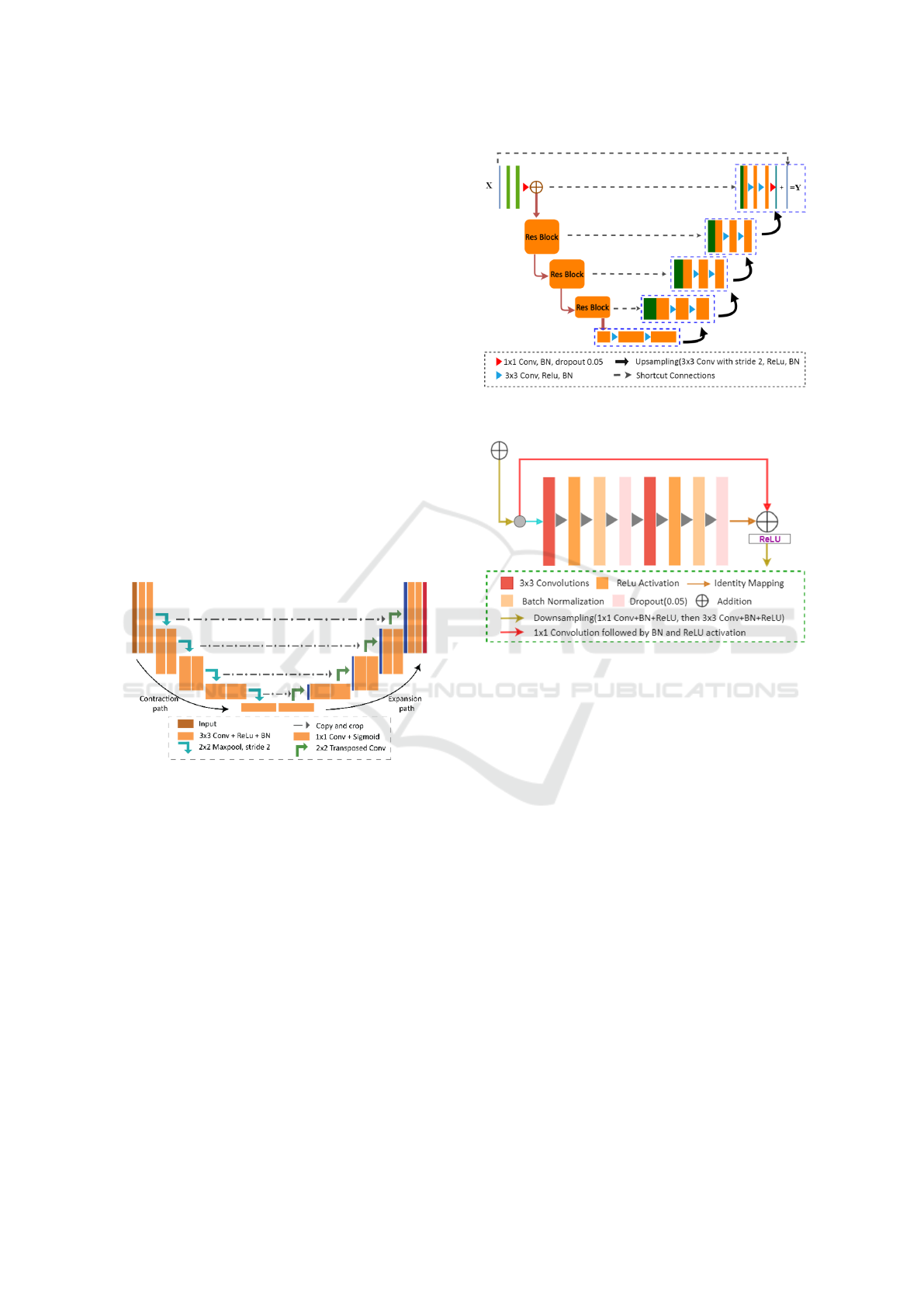
2.2.3 Residual UNet
After implementing and analyzing the UNet, the
recovered images exhibited a degree of over-
smoothness. To fix this, we improved the architecture
by adding residual blocks. These blocks stop degra-
dation by using skip connections within each block,
making it easier for low- and high-level features to
move across the network (He et al., 2016b).
The encoder captures feature maps from fine to
coarse scales, while the decoder up-samples these
maps with residual shortcuts in a coarse-to-fine man-
ner. In the Residual UNet, every two convolutional
layers in the original UNet are replaced with resid-
ual blocks, with 1x1 convolutions aligning the input-
Figure 3: Architectural Overview of the Residual UNet
(Res-UNet).
Figure 4: The block module consists of two 3x3 convo-
lutional layers, batch normalization, and ReLU activation,
with identity mapping for efficient feature propagation.
output feature channels, while all other parameters re-
main unchanged.
2.2.4 Fully Dense UNet
Modifying the UNet architecture with dense blocks
enables each layer to learn features at different spatial
scales, effectively reducing artifacts. The contract-
ing path of the Dense UNet repeatedly reduces spatial
dimensions using max-pooling (Guan et al., 2019).
In the expanding path, feature maps are upsampled
via deconvolution, concatenated with corresponding
feature maps from the encoding block, and then re-
fined with 1x1 convolutions before applying the dense
block. This dense connectivity enhances image re-
construction quality while reducing network parame-
ters, resulting in lower computational costs and faster
reconstruction.
The output of the dense block is concatenated with
all previous convolutional layers and learns features
in a ‘Collective knowledge’ manner through a se-
quence of 1x1 convolutional and 3x3 convolutional
followed by batch normalization and activation func-
VISAPP 2025 - 20th International Conference on Computer Vision Theory and Applications
376

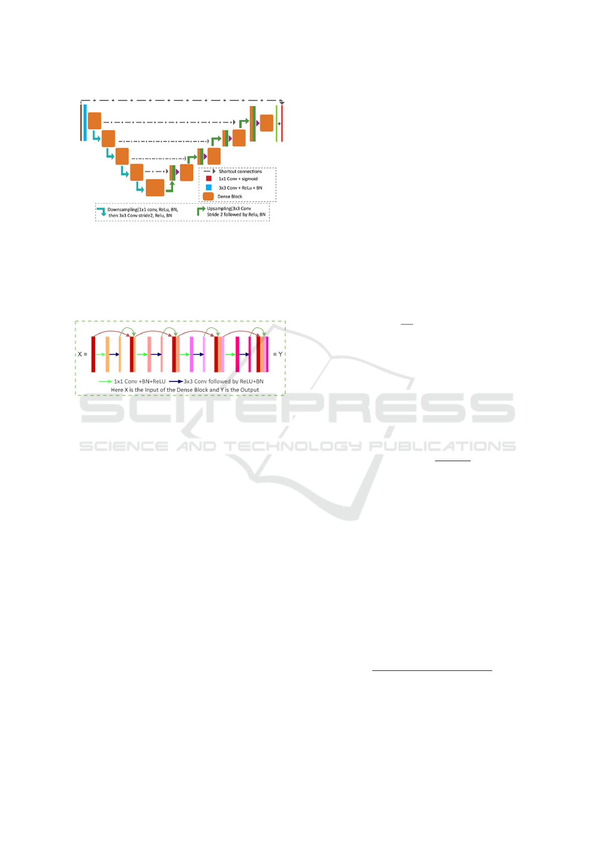
Figure 5: Illustration of the Modified Dense Block in the
UNet Architecture.
tion (ReLU). Without the vanishing gradient problem,
dense block allows deeper networks and improves
computational efficiency by applying 1x1 convolu-
tional to reduced feature-maps before 3x3 convolu-
tion.
Figure 6: In dense block, the feature of the previous layer is
concatenated together as the input of the following layer.
3 EXPERIMENTAL SETUP
3.1 Dataset and Training
To evaluate the performance of different Deep Convo-
lutional Neural Networks (DCNNs), we utilized the
MRNet dataset (Ramzi et al., 2020) from Stanford,
which contains knee MRI scans acquired in three
standard imaging planes: coronal, sagittal, and ax-
ial. Specifically, the T1-weighted sequences in the
coronal plane were used for this study. The MRNet
dataset comprises a series of images with an average
intensity mean and standard deviation of 31.48 and
7.97, respectively (Bien et al., 2018). However, some
images within the series reveal poor anatomical visi-
bility, which could impact training. These low-quality
images were removed as part of the data preprocess-
ing, resulting in a refined dataset. From the T1-
weighted coronal sequences, a total of 11,280 images
with a resolution of 256x256 pixels were extracted
from 1,370 knee MRI series. The models were trained
using the Adam optimizer with a learning rate of
0.0001 over 100 epochs for each undersampling ratio.
All neural networks were implemented using Python
3.7.8 with TensorFlow and PyTorch frameworks. The
training was conducted on a system equipped with 32
GB RAM and an NVIDIA V100 GPU with 12 GB of
memory.
3.2 Evaluation Metrics
To evaluate the performance of different deep learn-
ing models, different image quality assessment met-
rics are formulated, such as
3.2.1 Mean Square Error (MSE)
The MSE is the simplest and most complete reference
matrix approach used to assess the quality of the im-
age. To estimate the average squared difference be-
tween the predicted images and actual images, MSE
between two image matrices M and N is defined as:
MSE(M, N) =
1
AB
A−1
∑
i=1
B−1
∑
j=1
(M
i j
− N
i j
)
2
3.2.2 Peak Signal to Noise Ratio (PSNR)
It is mostly used to control the digital signal trans-
mission quality. PSNR is a variation of MSE that
strengthens the pixel-by-pixel comparison (Hore and
Ziou, 2010). To calculate the PSNR value between
the actual image A and reference image B with the
same size MxN is defined as,
PSNR = 10. log
10
max
2
image
MSE
!
The greater the PSNR value represents, the higher the
predicted image quality.
3.2.3 Structural Similarity Index Measure
(SSIM)
A well-known quality matrix is used to measure the
structural similarity between two images that gives
the normalized mean value. In the image domain,
the more important visual object information spatially
closed pixels refer to structure information (Hore and
Ziou, 2010). To calculate the image distortion, the
SSIM model used three factors such as loss of cor-
relation, luminance distortion, ad contrast distortion.
The simplified equation of SSIM is defined as,
SSIM(A,B) =
(2µ
A
µ
B
+C
1
)(2σ
AB
+C
2
)
(µ
2
A
+ µ
2
B
+C
1
)(σ
2
A
+ σ
2
B
+C
2
)
(10)
Here, µ
A
and µ
B
are the local means, σ
2
A
and σ
2
B
are
the variances, σ
AB
is the covariance, and C
1
and C
2
are constants used to stabilize the division. The SSIM
Learning-Based Reconstruction of Under-Sampled MRI Data Using End-to-End Deep Learning in Comparison to CS
377

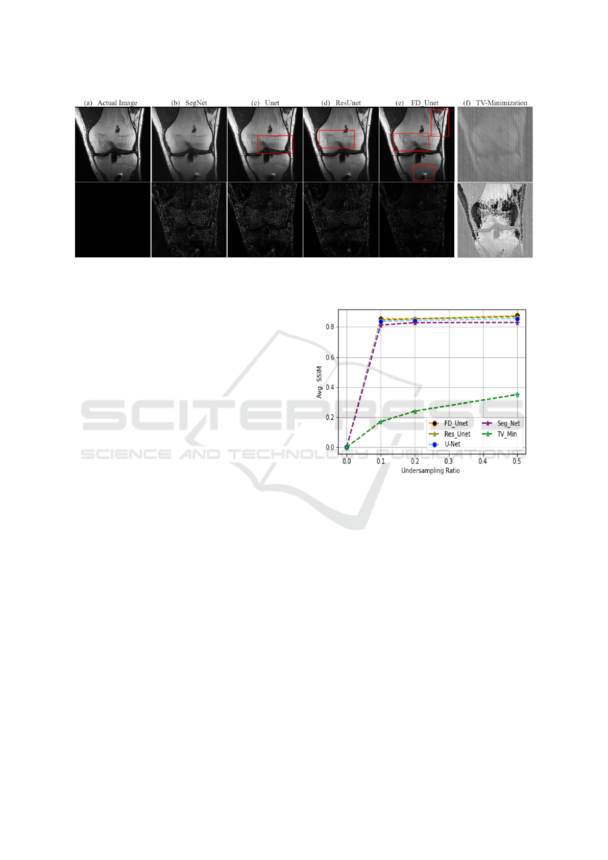
Figure 7: Comparison of reconstruction results for various models at an undersampling ratio of 0.5. The top row presents the
ground truth image alongside the predictions from different models, while the bottom row shows the difference maps between
the ground truth and predicted images, effectively highlighting the performance of each model.”.
index is within the range [0, 1], where 0 indicates no
correlation between the images and 1 indicates that
the actual image and predicted image are identical,
A = B.
4 RESULTS AND DISCUSSION
A comprehensive comparison of DL-based advanced
image reconstruction techniques is performed by tak-
ing the CS method as a baseline, as illustrated in Fig-
ure 7.
As envisaged, the DL methods are capable of re-
constructing artifactual data with high efficiency, tak-
ing into account features such as edges, luminance,
contrast, etc. The highlighted red box in Figure
7 visualizes that the proposed network not only re-
moves the under-sampled artifacts but also recovers
the minute details of the reconstructed images. In
essence, compared with other deep models, Fully
Dense UNet (FD-Unet) outperformed in recovering
fine details and reducing the over-smoothness ob-
served in images predicted by other methods even in
the least favorable scenarios (i.e., lowest sampling ra-
tio). On the other hand, CS-based TV minimization is
unable to recover the image with an acceptable diag-
nostic quality.
Taking into account the quantitative analysis,
based on the pre-defined evaluation metrics such as
average SSIM and PSNR, it can be seen in Figure
8 and 9 that CS-based TV minimization (sparsity-
based method) demonstrates the worst performance
with just SSIM = 0.314 and PSNR= 14.90dB even for
better working conditions such as undersampling ra-
tio of 0.5. Meanwhile, DL-based methods exhibit su-
perior performance, for instance, with an approximate
Figure 8: The average SSIM for the different undersampling
ratios between deep learning models and TV-Minimization.
average SSIM= 0.820−0.830 and PSNR = 24−26dB
for simple UNet, Residual UNet, SegNet under the
under-sampling ratio of just 0.2 (using 20% of the
total measurements). Additionally to highlight, as
discussed in qualitative discussion, UNet and SegNet
experience over-smoothing issue; however, the prob-
lem is not fully evident in quantitative analysis. Be-
sides FD-UNet outperformed all other methods hav-
ing SSIM = 0.84 and PSNR= 27 dB and significantly
reduces the over smoothing problem to a great extent
under the same undersampling conditions i.e. 0.2.
Providing further interpretation and wrapping up
the discussion, Figure 10 depicts the comparison of
each stage under a challenging scenario (using only
10% measurements) where the top row, (a) represents
the measurement image obtained with an undersam-
pling ratio of 0.1, and (b) shows the reconstructed im-
age predicted by the FD-UNet) model. Subsequently,
in the bottom row, (c) represents the actual ground
VISAPP 2025 - 20th International Conference on Computer Vision Theory and Applications
378

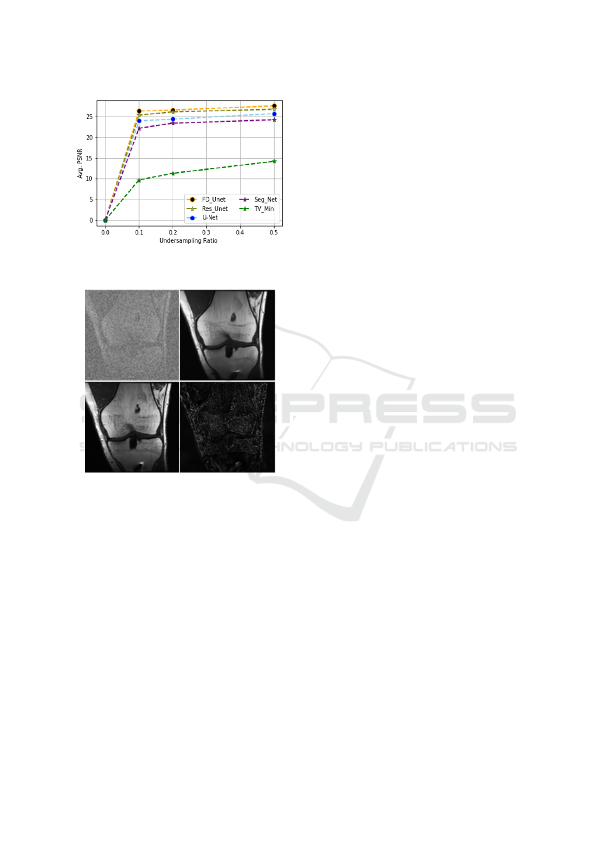
Figure 9: The average PSNR (db) for different sampling
ratio on test samples.
Input Image Predicted Image
Actual Image Difference
Figure 10: Predicted Results using 10% of actual image
data.
truth image, and (d) is the corresponding difference
between the FD-UNet predicted image and the ground
truth. In the predicted image, some over-smoothing is
identified, causing some details to be sacked.
Overall, in comparison to other neural networks,
UNet performs better and has the ability to recover
images but it is difficult to train and is vulnera-
ble to over-fitting due to integrated different layers.
The incorporation of the different residual blocks,
dense block, and inception block may help to im-
prove the performance. Here, in our scenario, the
dense block with skip connection improves the per-
formance in retrieving undersampled images because
more potential information and features are extracted
in the contracting path, and concatenating the feature
map learns more information from a different layer
of the network. Moreover, dense connection avoids
the learning of redundant features, enhances informa-
tion flow, and further reduces network parameters on
the premise of close performance. The reduction of
network parameters reduces the calculation cost, and
the image reconstruction can be faster. Overall, our
experiments showed that the recovery of real-world
medical data is possible using DL-based algorithms
with better diagnostic image quality and improved
performance in comparison with traditional CS-based
methods.
5 CONCLUSION AND FUTURE
WORKS
As recently, deep CNNs based networks are being
popular to remove artifacts and denoise the recon-
structed medical images. In this article, we com-
pare the performance of different deep-learning mod-
els with the help of synthetic data for real-world medi-
cal data image recovery without considering any con-
straints. The experimental results show that a fully
dense UNet has a better image-recovering effect un-
der the premise of fewer measurements. However,
these end-to-end recovering methods reconstruct the
image in just less than one second with the help of a
well-trained network. This method allows real-time
recovery of artifact images without delays. Future ef-
forts should focus on developing more advanced net-
works to capture finer details with lower computa-
tional costs. Additionally, refining existing architec-
tures or introducing new ones could lead to further
performance improvements.
ACKNOWLEDGMENT
This work was supported by the Bosomshield Project,
a grant from Marie Sklodowaka-Curie Doctoral
Networks Actions (HORIZON-MSCA-2021-DN-01-
01;101073222).
REFERENCES
Badrinarayanan, V., Kendall, A., and Cipolla, R. (2017).
Segnet: A deep convolutional encoder-decoder ar-
chitecture for image segmentation. IEEE transac-
tions on pattern analysis and machine intelligence,
39(12):2481–2495.
Bastounis, A. and Hansen, A. C. (2017). On the absence of
uniform recovery in many real-world applications of
compressed sensing and the restricted isometry prop-
erty and nullspace property in levels. SIAM Journal
on Imaging Sciences, 10(1):335–371.
Learning-Based Reconstruction of Under-Sampled MRI Data Using End-to-End Deep Learning in Comparison to CS
379

Bien, N., Rajpurkar, P., Ball, R. L., Irvin, J., Park, A., Jones,
E., Bereket, M., Patel, B. N., Yeom, K. W., Shpan-
skaya, K., et al. (2018). Deep-learning-assisted di-
agnosis for knee magnetic resonance imaging: devel-
opment and retrospective validation of mrnet. PLoS
medicine, 15(11):e1002699.
Brau, A. C., Beatty, P. J., Skare, S., and Bammer, R. (2008).
Comparison of reconstruction accuracy and efficiency
among autocalibrating data-driven parallel imaging
methods. Magnetic Resonance in Medicine: An Offi-
cial Journal of the International Society for Magnetic
Resonance in Medicine, 59(2):382–395.
Candes, E. J. (2008). The restricted isometry property and
its implications for compressed sensing. Comptes ren-
dus. Mathematique, 346(9-10):589–592.
Chen, H., Zhang, Y., Zhang, W., Liao, P., Li, K., Zhou, J.,
and Wang, G. (2017). Low-dose ct via convolutional
neural network. Biomedical optics express, 8(2):679–
694.
Feng, L., Benkert, T., Block, K. T., Sodickson, D. K., Otazo,
R., and Chandarana, H. (2017). Compressed sensing
for body mri. Journal of Magnetic Resonance Imag-
ing, 45(4):966–987.
Griswold, M. A., Blaimer, M., Breuer, F., Heidemann,
R. M., Mueller, M., and Jakob, P. M. (2005). Paral-
lel magnetic resonance imaging using the grappa op-
erator formalism. Magnetic resonance in medicine,
54(6):1553–1556.
Guan, S., Khan, A. A., Sikdar, S., and Chitnis, P. V. (2019).
Fully dense unet for 2-d sparse photoacoustic tomog-
raphy artifact removal. IEEE journal of biomedical
and health informatics, 24(2):568–576.
He, J., Liu, Q., Christodoulou, A. G., Ma, C., Lam,
F., and Liang, Z.-P. (2016a). Accelerated high-
dimensional mr imaging with sparse sampling using
low-rank tensors. IEEE transactions on medical imag-
ing, 35(9):2119–2129.
He, K., Zhang, X., Ren, S., and Sun, J. (2016b). Iden-
tity mappings in deep residual networks. In Computer
Vision–ECCV 2016: 14th European Conference, Am-
sterdam, The Netherlands, October 11–14, 2016, Pro-
ceedings, Part IV 14, pages 630–645. Springer.
Hore, A. and Ziou, D. (2010). Image quality metrics: Psnr
vs. ssim. In 2010 20th international conference on
pattern recognition, pages 2366–2369. IEEE.
Jin, K. H., McCann, M. T., Froustey, E., and Unser, M.
(2017). Deep convolutional neural network for in-
verse problems in imaging. IEEE transactions on im-
age processing, 26(9):4509–4522.
Lustig, M., Donoho, D., and Pauly, J. M. (2007). Sparse
mri: The application of compressed sensing for rapid
mr imaging. Magnetic Resonance in Medicine: An
Official Journal of the International Society for Mag-
netic Resonance in Medicine, 58(6):1182–1195.
Lustig, M., Donoho, D. L., Santos, J. M., and Pauly, J. M.
(2008). Compressed sensing mri. IEEE signal pro-
cessing magazine, 25(2):72–82.
Mousavi, A. and Baraniuk, R. G. (2017). Learning to
invert: Signal recovery via deep convolutional net-
works. In 2017 IEEE international conference on
acoustics, speech and signal processing (ICASSP),
pages 2272–2276. IEEE.
Provost, J. and Lesage, F. (2008). The application of com-
pressed sensing for photo-acoustic tomography. IEEE
transactions on medical imaging, 28(4):585–594.
Ramzi, Z., Ciuciu, P., and Starck, J.-L. (2020). Benchmark-
ing mri reconstruction neural networks on large public
datasets. Applied Sciences, 10(5):1816.
Ronneberger, O., Fischer, P., and Brox, T. (2015). U-
net: Convolutional networks for biomedical image
segmentation. In Medical image computing and
computer-assisted intervention–MICCAI 2015: 18th
international conference, Munich, Germany, October
5-9, 2015, proceedings, part III 18, pages 234–241.
Springer.
Sartoretti, E., Sartoretti, T., Binkert, C., Najafi, A.,
Schwenk,
´
A., Hinnen, M., van Smoorenburg, L.,
Eichenberger, B., and Sartoretti-Schefer, S. (2019).
Reduction of procedure times in routine clinical prac-
tice with compressed sense magnetic resonance imag-
ing technique. PloS one, 14(4):e0214887.
Wang, J., Zhang, C., and Wang, Y. (2017). A photoacoustic
imaging reconstruction method based on directional
total variation with adaptive directivity. Biomedical
engineering online, 16:1–30.
Wang, S., Su, Z., Ying, L., Peng, X., Zhu, S., Liang, F.,
Feng, D., and Liang, D. (2016). Accelerating mag-
netic resonance imaging via deep learning. In 2016
IEEE 13th international symposium on biomedical
imaging (ISBI), pages 514–517. IEEE.
Wang, W., Liang, D., Chen, Q., Iwamoto, Y., Han, X.-
H., Zhang, Q., Hu, H., Lin, L., and Chen, Y.-W.
(2020). Medical image classification using deep learn-
ing. Deep learning in healthcare: paradigms and ap-
plications, pages 33–51.
Ying, L., Haldar, J., and Liang, Z.-P. (2006). An efficient
non-iterative reconstruction algorithm for parallel mri
with arbitrary k-space trajectories. In 2005 IEEE En-
gineering in Medicine and Biology 27th Annual Con-
ference, pages 1344–1347. IEEE.
Zhang, H.-M. and Dong, B. (2020). A review on deep learn-
ing in medical image reconstruction. Journal of the
Operations Research Society of China, 8(2):311–340.
VISAPP 2025 - 20th International Conference on Computer Vision Theory and Applications
380