Curiosity Driven Reinforcement Learning for Job Shop Scheduling
Alexander Nasuta
a
, Marco Kemmerling
b
, Hans Zhou
c
, Anas Abdelrazeq
d
and Robert Schmitt
e
Chair of Intelligence in Quality Sensing, RWTH Aachen, Aachen, Germany
Keywords:
Curiosity, Reinforcement Learning, Job Shop Problem, Combinatorial Optimization.
Abstract:
The Job Shop Problem (JSP) is a well-known NP-hard problem with numerous applications in manufacturing
and other fields. Efficient scheduling is critical for producing customized products in the manufacturing in-
dustry in time. Typically, the quality metrics of a schedule, such as the makespan, can only be assessed after
all tasks have been assigned, leading to sparse reward signals when framing JSP as a reinforcement learning
(RL) problem. Sparse rewards pose significant challenges for many RL algorithms, often resulting in slow
learning behavior. Curiosity algorithms, which introduce intrinsic reward signals, have been shown to acceler-
ate learning in environments with sparse rewards. In this study, we explored the effectiveness of the Intrinsic
Curiosity Module (ICM) and Episodic Curiosity (EC) by benchmarking them against state-of-the-art methods.
Our experiments demonstrate that the use of curiosity significantly increases the amount of states encountered
by the RL agent. When the intrinsic and extrinsic reward signals are of comparable magnitude, the agent is
with ICM module are able to escape local optima and discover better solutions.
1 INTRODUCTION
Production planning is a critical challenge across in-
dustries, with resource allocation and task schedul-
ing being complex decisions. The Job Shop Prob-
lem (JSP) is particularly relevant in manufacturing,
where efficient scheduling is essential for produc-
ing customized products and managing small batches
(Bła
˙
zewicz et al., 2019). In a JSP, each product
is treated as a job consisting of tasks that must be
processed on specific machines in a particular order.
This flexibility makes JSP widely applicable but also
highly complex, as it is an NP-hard problem, meaning
that finding exact solutions is computationally infea-
sible for large instances. To tackle this complexity,
heuristic and metaheuristic approaches are often used
to find near-optimal solutions. Recently, reinforce-
ment learning (RL) has emerged as a promising ap-
proach, allowing agents to learn adaptive scheduling
heuristics through interaction with the environment.
However, applying RL to JSPs poses challenges, par-
ticularly due to the sparse reward structure. In JSP,
a
https://orcid.org/0009-0007-5111-6774
b
https://orcid.org/0000-0003-0141-2050
c
https://orcid.org/0000-0002-7768-4303
d
https://orcid.org/0000-0002-8450-2889
e
https://orcid.org/0000-0002-0011-5962
the quality of a schedule is typically assessed only af-
ter all tasks are scheduled, leading to delayed rewards
and a slow learning process.
One of the key issues in RL is the exploration-
exploitation dilemma, where the agent must balance
trying new actions (exploration) with using known
successful actions (exploitation). This dilemma is es-
pecially problematic in sparse reward environments
like JSPs, where it’s difficult for the agent to identify
which actions contributed to success or failure.
Curiosity-based exploration algorithms offer a so-
lution approach by introducing intrinsic rewards that
encourage the agent to systematically explore new
states or actions, even without immediate external re-
wards. This approach has been shown to acceler-
ate learning in various RL tasks, particularly in en-
vironments with sparse rewards (Pathak et al., 2017;
Savinov et al., 2018). Despite its potential, curiosity-
driven exploration has not been widely studied in the
context of JSPs to the best of our knowledge.
This research aims to explore the impact of
curiosity-based exploration on RL agents in a job
shop environment. By integrating curiosity algo-
rithms into a typical RL setup, we seek to improve
the effectiveness of scheduling solutions.
216
Nasuta, A., Kemmerling, M., Zhou, H., Abdelrazeq, A. and Schmitt, R. H.
Curiosity Driven Reinforcement Learning for Job Shop Scheduling.
DOI: 10.5220/0013143800003890
Paper published under CC license (CC BY-NC-ND 4.0)
In Proceedings of the 17th International Conference on Agents and Artificial Intelligence (ICAART 2025) - Volume 2, pages 216-227
ISBN: 978-989-758-737-5; ISSN: 2184-433X
Proceedings Copyright © 2025 by SCITEPRESS – Science and Technology Publications, Lda.

2 RELATED WORK
This section provides an overview of the existing lit-
erature on curiosity algorithms in RL and the appli-
cation of RL to the JSP. It is divided into two sub-
sections: Curiosity Algorithms in RL, which explores
various approaches to intrinsic motivation in RL, and
RL approaches for the JSP, which reviews how RL
has been applied to solve JSP instances.
2.1 Curiosity Algorithms in RL
Curiosity-driven exploration has emerged as a possi-
bility to guide RL agents to explore the state space
in a systematic way in environments with sparse re-
wards. The primary challenge in sparse reward en-
vironments is the exploration-exploitation dilemma,
where an agent must decide between exploring new
actions or exploiting known successful actions. While
this dilemma holds true for any RL setting it is es-
pecially severe, where rewards are infrequent or de-
layed, leading to slow and inefficient learning. To
address this challenge, curiosity algorithms introduce
intrinsic rewards, which encourage an agent to ex-
plore states or actions that are novel or uncertain, even
in the absence of external rewards.
One of the simplest curiosity mechanisms is
count-based curiosity, where the agent receives
higher rewards for visiting less-explored states. The
method’s limitation lies in its infeasibility for envi-
ronments with a vast state space. Bellemare et al.
(2016) addressed this issue by introducing pseudo-
counts, which estimate state visitation counts using
a neural network, thereby enabling more efficient ex-
ploration in complex environments like Atari games.
Prediction-based curiosity, initially proposed by
Schmidhuber (1991), is another prominent approach.
It involves the agent predicting the next state based
on the current state and action, with the intrinsic re-
ward being the prediction error. This method al-
lows the agent to focus on learning areas of the en-
vironment where its predictive model is less accu-
rate, fostering more efficient exploration. Pathak et al.
(2017) enhanced this approach with the Intrinsic Cu-
riosity Module (ICM), which transforms states into
a feature space to filter out statistic noise. The ICM
has demonstrated significant improvements in learn-
ing efficiency in sparse reward environments like Viz-
Doom and Super Mario Bros compared to approaches
without a curiosity approach.
Episodic Curiosity (EC), introduced by Savinov
et al. (2018), suggest a different concept of curios-
ity by defining novelty in terms of the agent’s abil-
ity to reach a new state from previously encountered
states within a limited number of actions. If a state is
deemed novel, it is stored in memory, and the agent
is rewarded, thus promoting exploration of genuinely
new areas of the environment. EC has shown su-
perior performance in environments like VizDoom,
DM-Lab, and MuJoCo, outperforming the ICM in the
evaluated use cases.
2.2 RL Approaches for the JSP
The Job Shop Problem is a classic combinatorial op-
timization problem, widely recognized for its com-
putational complexity as an NP-hard problem. The
goal in JSP is to determine an optimal schedule for
a set of jobs, each consisting of multiple tasks that
must be processed on specific machines in a prede-
fined order. Given its complexity, JSP has tradition-
ally been addressed using heuristic and metaheuristic
approaches. However, with recent advances in rein-
forcement learning, RL has emerged as a promising
tool for solving JSPs.
Samsonov et al. (2021) introduced a reinforce-
ment learning framework that utilizes a sparse re-
ward function for JSP. In this approach, a discrete
time simulation of the job shop environment is em-
ployed, where an RL agent assigns tasks to machines.
The reward is sparse, provided only at the end of the
scheduling process, and is inversely proportional to
the makespan. This method allows the agent to focus
on achieving near-optimal schedules but faces chal-
lenges due to the delayed nature of the reward.
In contrast, Tassel et al. (2021) proposed a dense
reward function for JSP that is based on machine uti-
lization. Here, the reward at each time step is de-
termined by the area occupied by tasks in the Gantt
chart and the extent of idle times. By optimizing the
scheduled area, this method indirectly minimizes the
makespan, allowing for more frequent rewards and
thus faster learning.
Zhang et al. (2020) took a different approach by
modeling the JSP as a disjunctive graph. The RL
agent uses a graph neural network (GNN) to trans-
form states into a latent space. The reward function
in this model is based on the critical path in the dis-
junctive graph, allowing the agent to adapt to JSP in-
stances of varying sizes. This method has demon-
strated the ability of RL agents to generalize across
different JSP scenarios, offering a scalable solution to
the problem.
Nasuta et al. (2023) introduced a highly config-
urable RL environment, adhering to the Gym stan-
dard
1
, aimed at JSPs. The study compared various
1
https://www.gymlibrary.dev/index.html
Curiosity Driven Reinforcement Learning for Job Shop Scheduling
217

reward functions, including sparse and dense formu-
lations. While no single reward function emerged
as universally superior across a wide range of JSP
instances, dense reward functions based on machine
utilization, such as those proposed by Tassel et al.
(2021), tended to optimize the makespan more ef-
fectively than sparse rewards that target makespan
directly. These findings suggest that dense reward
signals can provide more consistent learning signals,
leading to improved scheduling performance.
Recent approaches have also explored the combi-
nation of RL with Monte Carlo Tree Search (MCTS),
a heuristic search method originally developed for
combinatorial games. MCTS represents the solu-
tion space as a tree and employs random sampling
to guide search efforts. Algorithms that combine RL
with MCTS, often referred to as neural MCTS, have
been notably applied in high-profile examples like Al-
phaGo and AlphaZero (Kemmerling et al., 2024b).
Oren et al. (2021) introduced an approach that in-
tegrates Deep Q-Learning for policy training in an
RL setting but incorporates MCTS during production
runs to generate superior solutions compared to rely-
ing solely on the learned policy.
Kemmerling (2024) explored in which cases neu-
ral MCTS outperforms conventional model-free rein-
forcement learning by analyzing job and operation di-
versity using Shannon entropy. Datasets with vary-
ing entropy levels were generated to assess each ap-
proach’s performance under different problem com-
plexities. The results showed that while model-free
agents struggled with high-entropy instances, neural
MCTS could overcome this challenge by performing
additional planning during decision-making, leading
to solutions closer to the optimal even in more diverse
and complex scheduling scenarios.
While RL approaches have shown promising re-
sults, they are prone to learn policies that result in lo-
cal optima, leaving room for improvement. Sparse
rewards, in particular, remain a significant challenge.
We aim to address this by integrating curiosity-based
algorithms into the RL framework for JSP, with the
goal of investigating the learning efficiency and solu-
tion quality of curiosity-based algorithms.
3 METHODOLOGY
This section introduces the underling optimization
problem of a JSP and outlines the methodology used
in our study, focusing on the design of a JSP envi-
ronment as a Markov Decision Process (MDP) and
the experimental setup employed to evaluate two
curiosity-driven exploration algorithms: ICM intro-
duced by Pathak et al. (2017) and EC introduced by
Savinov et al. (2018).
JSP Formalization. The JSP is a classical schedul-
ing problem where a set of tasks T = {T
1
, T
2
, . . . , T
N
}
must be processed on a set of machines M = {M
i
}
m
i=1
.
Each job, representing the production of a specific
product, is composed of a sequence of tasks, with
each task corresponding to a specific production step.
The problem considers a set of jobs J = {J
j
}
n
j=1
,
where the total number of tasks N is determined by
the number of jobs n and the number of machines m,
such that N = n · m. A solution to the JSP, a feasible
schedule, assigns a start time ˆs
α
to each task T
α
, while
ensuring that the precedence constraints and machine
availability constraints are not violated. Our work
leverages a disjunctive graph approach to model the
JSP, like Zhang et al. (2020) and Nasuta et al. (2023).
In this approach, the disjunctive graph G consists of
a set of nodes V , directed edges A, and undirected
edges E. The set of nodes V includes the tasks T
and two fictitious nodes, the source T
0
and the sink
T
⋆
, such that V = T ∪{T
0
, T
⋆
}. The directed edges A,
termed conjunctive edges, represent precedence rela-
tions and are initially derived from the sequence of
tasks within each job. The undirected edges, known as
disjunctive edges, are introduced between tasks that
require the same machine, reflecting the yet unde-
cided order of processing on that machine. To gen-
erate a valid schedule, all disjunctive edges must be
directed in such a way that the resulting graph re-
mains acyclic. The makespan, defined as the total
time required to complete all jobs, can be determined
by finding the longest path, also known as the critical
path, from T
0
to T
⋆
in the fully scheduled graph.
The discrete optimization problem for minimizing
the makespan can be formally stated as follows: Min-
imize s
⋆
subject to (Bła
˙
zewicz et al., 2019):
ˆs
β
− ˆs
α
≥ p
α
∀ (T
β
, T
α
) ∈ A (1)
ˆs
α
≥ 0 ∀ T
α
∈ T (2)
ˆs
β
− ˆs
α
≥ p
α
∨ ˆs
α
− ˆs
β
≥ p
β
∀ {T
β
, T
α
} ∈ E
i
, (3)
∀ M
i
∈ M
Markov Decision Process. In this study the JSP is
modelled as a Markov Decision Process to facilitate
the training of RL agents. The state space spans all
possible configurations of the partial schedule, while
the action space consists of choices regarding which
job’s next unscheduled operation to schedule.
Observation Space. For a RL setup the state rep-
resentation needs to encode all information of a par-
ICAART 2025 - 17th International Conference on Agents and Artificial Intelligence
218

0
1 2
3
4
5 6
7
8
⋆
0
0
11 3 3
12
5 16
7
4
(a) Initial disjunctive graph.
0
1 2
3
4
5 6
7
8
⋆
0
0
11 3 3
12
5 16
7
4
5
(b) Partially scheduled graph.
0
1 2
3
4
5 6
7
8
⋆
0
0
11 3 3
12
5 16
7
4
5
3
16
12
(c) Fully scheduled disjunctive graph with high-
lighted critical path.
0
1 2
3
4
5 6
7
8
⋆
0
0
11 3 3
12
5 16
7
4
5
3
16
(d) Infeasible schedule with highlighted cycle.
Figure 1: Disjunctive graph scheduling.
tial solution. When formulating the JSP using a dis-
junctive graph approach, any that alows to construct
graphs, such as seen in Figure 1a- 1c is a valid state
representation. We represent the graph by an adja-
cency matrix, that is extended with columns for the
machine and the processing duration of a task. The
state representation corresponding to Figure 1b is pro-
vided in the appendix, in Table 3.
Action Space. The action space consists of the set
off all tasks along with an action mask, that masked
out actions that might lead to infeasible schedules.
In our setup tasks within a job are scheduled left to
right similar to Zhang et al. (2020) and Nasuta et al.
(2023), which ensures an acyclic graph at any point in
time. For the instance in Figure 1 consits of the tasks
{t
1
,t
2
, ...,t
8
}. Valid actions in Figure 1a are {t
1
,t
5
}.
In Figure 1b {t
2
,t
6
} are valid actions.
Reward Function. The reward function is a sparse
reward function incentivizes actions that minimize the
makespan:
r(s
t
) =
(
−
C
C
LB
end of episode
0 otherwise
(4)
C
LB
denotes a lower bound of the makespan for a spe-
cific instance. Therefore the reward is always in the
same range across different instances. If C
LB
equals
the optimal makespan, the reward r will approach −1
as the agent finds better and better solutions. This re-
ward function was introduced by Nasuta et al. (2023)
as a trivial reward function, due to its simplicity. De-
spite Nasuta et al. (2023) incentives to formulate a
dense reward function based on the machine utiliza-
tion, we chose to use a sparse reward function to study
the effects of curiosity algorithms, because curiosity
was specifically introduced to excel on enviornments
with a sparse reward structure.
Curiosity Algorithms. We consider the ICM ap-
proach by Pathak et al. (2017) and the EC approach
introduced by Savinov et al. (2018) in our work, since
these approaches are the most advanced curiosity al-
gorithms demonstrating the best performance scoring
in the domain of Atari games with sparse rewards.
The following paragraphs cover both approaches in
more detail.
Intrinsic Curiosity Module. The ICM, as intro-
duced by Pathak et al. (2017), is an approach de-
signed to address the challenge of sparse reward en-
vironments in reinforcement learning. It builds on the
concept of intrinsic motivation by generating rewards
based on the agent’s inability to predict the outcomes
of its actions, encouraging exploration in uncertain re-
gions of the environment. The ICM operates by trans-
forming raw states s
t
and s
t+1
into a feature space
φ(s
t
), φ(s
t+1
), to reduce the influence of stochastic
noise in the environment. The forward model predicts
the next state in the feature space, and the intrinsic re-
ward is calculated as the error between the predicted
and actual subsequent state


ˆ
φ(s
t+1
) − φ(s
t+1
)


. This
reward drives the agent to explore areas where its pre-
dictions are less accurate. Additionally, the ICM in-
cludes an inverse model, which predicts the action
taken by the agent based on the feature representa-
tion of the current and next state. This ensures that
the feature space captures relevant dynamics, filtering
out noise. The combination of the forward and inverse
models is optimized using a shared optimizer, with a
weighted sum of their errors guiding the network pa-
rameters.
Curiosity Driven Reinforcement Learning for Job Shop Scheduling
219

−
φ
Forward
Model
Inverse
Model
a
t
s
t
s
t+1
φ(s
t
)
φ(s
t+1
)
ˆ
φ(s
t+1
)
ˆa
t
r
in
t+1
Figure 2: Signal block diagram for the ICM.
Episodic Curiosity. The Episodic Curiosity Mod-
ule (EC), proposed by Savinov et al. (2018), provides
a mechanism for detecting novelty in an agent’s envi-
ronment by comparing the agent’s current state to pre-
viously encountered states stored in a memory buffer.
Novelty, in this context, is defined by how many ac-
tions are required to move from a known state to the
current state. Specifically, if more than a predefined
number of actions, k, are needed to reach the current
state s
t
from any state in the memory buffer M, the
state is considered novel and an intrinsic reward is
generated. The EC utilizes two neural networks: an
embedding network E, which transforms the current
state s
t
into a feature space E(s
t
), and a comparator
network C, which estimates the reachability of s
t
from
stored states s
m
∈ M. The comparator C predicts a
continuous reachability score between 0 and 1, with 1
indicating that s
t
is reachable within k actions. These
predictions form a reachability buffer R, which is then
aggregated into a scalar value using a function F, typ-
ically set as the 90th-percentile to account for neural
network approximation errors. This scalar is passed
to a bonus function B, and if the resulting value b ex-
ceeds a novelty threshold b
novelty
, the state is deemed
novel, and E(s
t
) is added to the memory buffer. The
intrinsic reward r
in
t+1
is set to b when novelty is de-
tected, or 0 otherwise. The shown in Figure 3 in this
paper illustrates the interaction between these compo-
nents and the flow of information within the EC sys-
tem.
Embedding
network
Comparator
network
Reach-
ability
buffer
F B
Memory
buffer
append E(s
t
) to
Memory buffer,
if b > b
novelty
s
t
r
in
t+1
E(s
t
)
E(s
m
)
R
F(R)
b
Figure 3: Signal block diagram for the EC.
3.1 Experimental Setup
This section covers the details on the experiment de-
sign and the on the specific software and frameworks
used in this study. First the details on the implemen-
tation of of the investigated curiosity algorithms are
covered, then we highlight or RL setup and the used
libraries for RL and Experiment tracking.
Curiosity Module Implementation. We consider
implementations of the ICM and EC within the rein-
forcement learning (RL) frameworks RLlib
2
and Sta-
ble Baselines3 Contrib (SB3)
3
. RLlib provides an im-
plementation of ICM that can be integrated into an RL
setup via its exploration API. We implemented EC
using RLlib’s exploration API and validated it with
the FrozenLake environment test cases, similar to the
validation process used for RLlib’s ICM implemen-
tation. For the SB3 approach, we implemented both
ICM and EC in the form of Gymnasium wrappers and
evaluated the implementations in the FrozenLake en-
vironment. The metrics for these evaluation test cases
are available on the Weights and Biases (WandB) plat-
form
45
.
Reinforcement Learning Setup. This study uti-
lizes the Gymnasium environment introduced by Na-
suta et al. (2023), which was configured to realise the
Observation and Action space described above along
with the described sparse reward function. The cu-
riosity modules in our setup are realised as gymna-
sium wrappers. For experiment tracking we use the
WandB plattform. After the validation of our curios-
ity implementations, we decided to use the SB3 setup
for the evaluation curiosity algorithms on the JSP, be-
cause in is more convenient to realize action masking
and incorporate custom WandB metrics. We consider
the metrics described in Table 1 in our experiments:
The Proximal Policy Optimization (PPO), originally
proposed by Schulman et al. (2017), algorithm was
chosen as the baseline reinforcement learning algo-
rithm for this study. PPO, a robust and efficient actor-
critic method, is well-suited for tasks with complex
action spaces like JSP.
Hardware. All computations in this study were per-
formed on an Apple Macbook Pro with a M1 Max
chip with 64 Gb of shared memory.
2
https://docs.ray.io/en/latest/rllib/index.html
3
https://sb3-contrib.readthedocs.io/en/master/
4
https://wandb.ai/querry/frozenlake-ray
5
https://wandb.ai/querry/frozenlake-sb3
ICAART 2025 - 17th International Conference on Agents and Artificial Intelligence
220

Table 1: Experiment Metrics.
Metric Fromula Description
extrinsic return G
ex
The return resulting from the environment
intrinsic return G
int
The return resulting from the investigated curiosity module
total return G
total
= G
ex
+ G
int
The sum of intrinsic and extrinsic return.
visited states
∥
S
∥
The number of distance states the agent encountered.
loss L
The loss from the optimiser, that trains the trains the neural
network inside a curiosity module
3.2 Experiment Design
There are two main approaches in the literature for
solving the JSP using RL. The first approach aims to
find the best possible solution for a specific instance
within a given time budget, as explored by Tassel et al.
(2021) and Kemmerling et al. (2024a). The second
approach seeks to train an agent on a variety of in-
stances, with the goal of generalizing to solve any new
instance, as pursued by Zhang et al. (2020).
In this work, we focus on solving individual in-
stances of the JSP. The source code for our experi-
ments is available on GitHub
6
.
For evaluating the impact of curiosity modules in
a RL setup for the JSP we utilize the well-known
benchmark JSP instances from Fisher (1963): ft06,
an instance with 6 jobs and 6 machines (size 6 × 6),
and ft10, an instance with 10 jobs and 10 machines
(size 10 × 10). These instances represent a range of
complexities, with ft06 being smaller and less com-
putationally demanding, while ft10 presents a more
challenging scheduling scenario due to its larger size.
The environment was configured with a sparse reward
function, as described above, providing feedback only
upon completion of a full schedule, thus creating a
challenging exploration scenario ideal for evaluating
curiosity-driven algorithms. To ensure that the PPO
algorithm was well-tuned for each JSP instance size,
a hyperparameter tuning process was conducted us-
ing the sweep functionality of WandB. The tuning fo-
cused on parameters such as the discount factor, neu-
ral network architecture, whether to turn off the intrin-
sic reward signal at some point and hyperparameters
of the curiosity modules. An exhaustive list of the
resulting parameters is provided in the appendix.
We divided the hyperparameter tuning process for
the ft06 instance into two stages. In the first stage,
we performed hyperparameter tuning using randomly
selected hyperparameters. Subsequently, we con-
ducted a grid search over the parameters of the best-
performing runs from the first stage. For the ft06
instance, we applied this two-stage process to three
6
https://github.com/Alexander-Nasuta/
Curiosity-Driven-RL-for-JSP
setups: a plain PPO, a PPO with an ICM, and a
PPO with EC. The first stage consisted of 300 runs,
each with 75k timesteps, followed by the second
stage with 192 runs, each with 50k timesteps. In
total, 1, 504 hyperparameter tuning runs were com-
pleted. For each setup (PPO, PPO with ICM, and PPO
with EC), the best-performing hyperparameter con-
figuration—resulting in the lowest makespan—was
further evaluated over 10 runs with a budget of 500k
timesteps.
For the ft10 instance, we performed 100 runs
for the plain PPO and 49 runs for the ICM, both
with randomly chosen hyperparameters and 1 mil-
lion timesteps. After 500k timesteps, ICM explo-
ration was turned on during hyperparameter tuning.
The best-performing PPO configuration was selected
as the baseline. Two ICM configurations were chosen
for further evaluation: one that resulted in the lowest
makespan and one that explored the highest number
of states. Due to computational challenges, we de-
cided to exclude the EC module in the larger-scale 10
× 10 scenario.
4 RESULTS AND DISCUSSION
This section presents the key findings of the experi-
ments and provides a discussion of the outcomes. All
recorded metrics are publicly available on WandB
7
.
The best performing hyperparameter configura-
tions for ft06 can be found for PPO, PPO with ICM
and PPO with EC in Listings 1, 2 and 3, respectively.
The performance of the agent in evaluation runs after
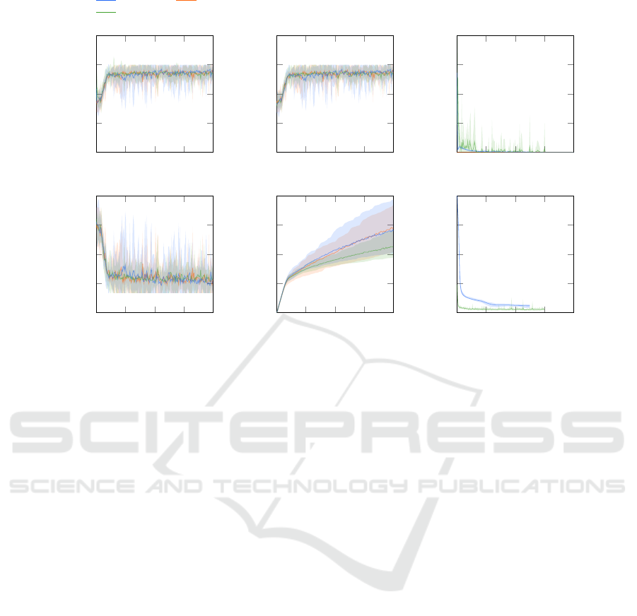
hyperparameter tuning is visualized in Figure 4.
There are no significant differences in extrinsic re-
turns or makespan among the evaluated groups. The
performance of the PPO agent and the PPO agent with
ICM is quite similar in terms of visited states. The
PPO with the EC module visits slightly fewer states
on average but remains largely within the range of the
PPO and PPO with ICM. This difference is likely due
to statistical fluctuations.
7
https://wandb.ai/querry/MA-nasuta
Curiosity Driven Reinforcement Learning for Job Shop Scheduling
221

PPO with ICM
PPO with EC
PPO without curiosity
0 250 500
-0.75
-1.25
-1.75
timesteps [k]
G
total
[1]
0 250 500
-0.75
-1.25
-1.75
timesteps [k]
G
ex
[1]
0 250 500
0
0.1
0.2
timesteps [k]
G
in
[1]
0 250 500
50
65
80
timesteps [k]
makespan [1]
0 250 500
0
50
100
timesteps [k]
∥
S
∥
[k]
0 250 500
0
1.5
3
timesteps [k]
loss [1]
Figure 4: Evaluation runs on the ft06 instance.
No significant differences were observed between
the baseline PPO and the PPO variants with curios-
ity modules, given the selected parameterizations. A
possible explanation for this is the relatively low scale
of the intrinsic reward signal, which might be too
small to significantly influence the agent’s behavior.
As shown in Figure 4, the intrinsic rewards are one
to two orders of magnitude lower than the extrinsic
rewards, making the intrinsic reward function more
akin to noise than a meaningful goal-directed signal.
Additionally, we observed a considerable increase
in computational demand when incorporating the EC
module. This is due to the EC requires a prediction for
every entry in the memory buffer at each timestep, in
contrast to the ICM, which only requires two predic-
tions per timestep. Another contributing factor to the
increased computation is that our implementation of
EC utilizes native Python data structures, rather than
optimized implementation for managing the memory
buffer, as used in the original implementation by Savi-
nov et al. (2018). Due to these computational chal-
lenges, we decided to exclude the EC module in the
larger-scale 10 × 10 scenario.
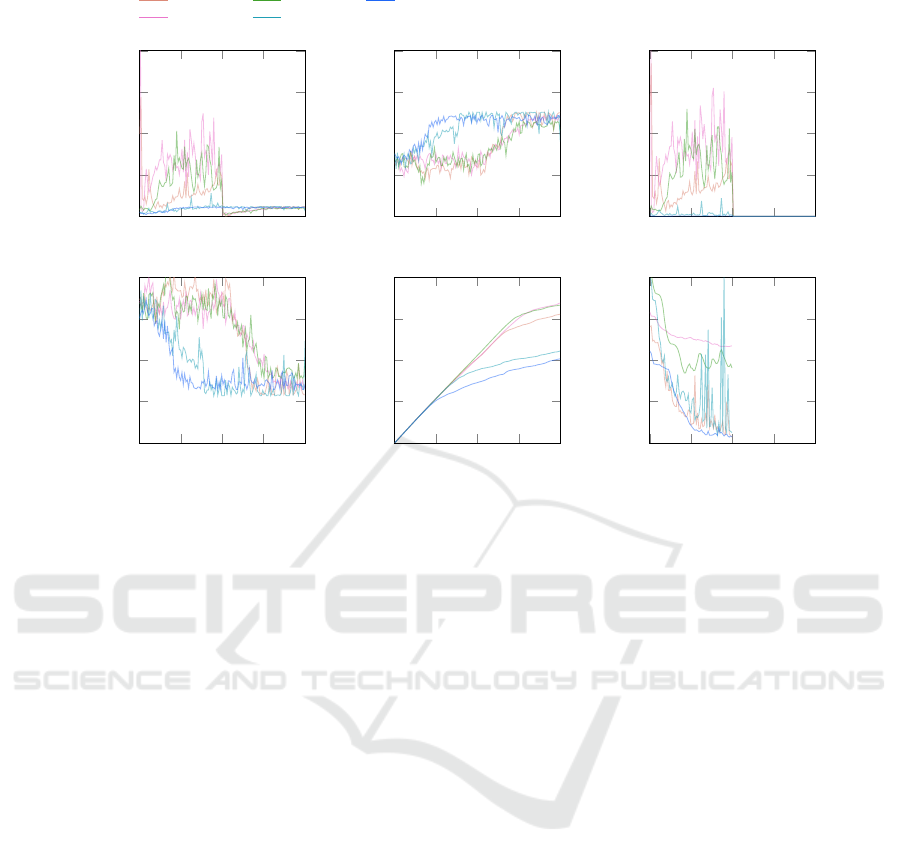
The 10 × 10 sized JSPs are significantly more
complex than 6×6 sized ones, making them more ap-
propriate for evaluating the impact of curiosity. Fig-
ure 5 presents selected runs form the hyperparameter
tuning on the ft06 instance that illustrate how intrinsic
curiosity affects scheduling.
Runs with high intrinsic rewards (pink shades
in Figure 5) exhibit noticeably different behavior
from those with low intrinsic rewards (green and
blue shades). With low intrinsic rewards, agent be-
havior is similar to that without the ICM module,
with the makespan dropping quickly and stabilizing
and low exploration. In contrast, high intrinsic re-
wards initially result in more exploration and higher
makespans. After 500k steps, the ICM is turned off
in all runs, causing intrinsic rewards to drop to zero.
Immediately afterward, the makespans of the green
curves improve, indicating a shift from exploration to
exploitation.
Higher intrinsic rewards clearly lead to increased
exploration, while low intrinsic rewards appear to act
as noise, with little impact on behavior. In the case of
an ICM, the intrinsic reward is the prediction error for
the next state, scaled by the parameter η. Hence, η is
crucial in determining the magnitude of the intrinsic
reward signal. Models with poor predictions generate
higher intrinsic rewards, driving more exploration.
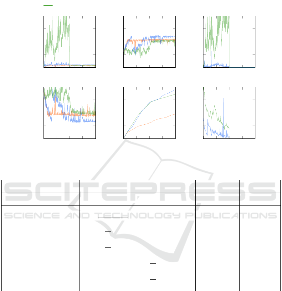
For the comparison between plain PPO and PPO
with ICM, two runs from the ICM hyperparame-
ter tuning were selected: the best-performing run
(kind-sweep-18 with η = 0.0276) and the run with
the highest level of exploration (still-sweep-27
with η = 0.0615). In the following, we refer to PPO
with ICM parameterized as kind-sweep-18 as setup
I, PPO with ICM parameterized as still-sweep-27
as setup II, and PPO without curiosity-driven explo-
ICAART 2025 - 17th International Conference on Agents and Artificial Intelligence
222

η = 0.6612
η = 0.4850
η = 0.06152
η = 0.01067
η = 0.001138
0 0.5 1
-1.5
1.75
5
timesteps [m]
G
total
[1]
0 0.5 1
-0.75
-1.25
-1.75
timesteps [m]
G
ex
[1]
0 0.5 1
0
2.5
5
timesteps [m]
G
in
[1]
0 0.5 1
900
1150
1400
timesteps [m]
makespan [1]
0 0.5 1
0
400
800
timesteps [m]
∥
S
∥
[k]
0 0.5 1
0
2
4
timesteps [m]
loss [1]
Figure 5: Selected hyperparameter tuning runs for a PPO with ICM on the ft10 instance.
ration as setup III. Both curiosity setups were com-
pared to a PPO agent without curiosity, using 4m
timesteps. These resulting runs are illustrated in Fig-
ure 6.
Setup II has a low η of 0.0615 but high, fluctu-
ating intrinsic rewards due to large prediction errors
from the ICM model. In contrast, Setup I achieved the
lowest makespan, with intrinsic rewards ranging from
0.1 to 0.3 and less fluctuation. These variations likely
stem from differences in the complexity of the inter-
nal neural networks, with Setup I having more layers
and nodes than Setup II. After 2m timesteps, the ICM
was switched off. Figures 6 shows that agents with
ICM explore significantly more states pairs than PPO
without curiosity in setup III. The makespan of Setup
II remains high while the ICM is active, but improves
after it is turned off. Across all setups, the makespan
improves initially but eventually reaches a plateau.
Periods of decreasing makespan correspond with high
exploration rates, while stagnation in the makespan is
associated with reduced exploration. Setup I suggests
that a well-tuned ICM can drive exploration into new
regions, potentially breaking out of local minima.
A comparison to other approaches found in the lit-
erature is presented in Table 2. This table also in-
cludes specific run names that can be used to locate
the corresponding experiments on the WandB plat-
form. Our setup I slightly outperforms other dis-
junctive graph-based methods, such as the trivial and
graph-tassel approaches proposed by Nasuta et al..
However, the time-based approach introduced by Tas-
sel et al. performs significantly better than both our
method and the other disjunctive graph approaches
examined in Nasuta et al. (2023). Nasuta et al. con-
cluded that a dense reward function based on ma-
chine utilization is most effective for solving Job
Shop Scheduling Problems (JSPs) using reinforce-
ment learning. Our results suggest that introducing
curiosity into a disjunctive graph-based approach of-
fers only marginal improvements, while requiring ad-
ditional computational resources for calculating the
intrinsic reward and training the neural networks in
the curiosity module. The tassel approach demon-
strates that a lower makespan can be achieved by
leveraging machine utilization to densify the reward
structure in JSPs. We presume that, although curios-
ity can help escape local minima, a reward structure
based on machine utilization is more likely to yield
better results when computational resources are con-
strained. This is because it enables more timesteps
within a given timeframe, avoiding the overhead in-
troduced by the intrinsic curiosity signal.
5 CONCLUSION
Our experiments demonstrate that the use of curiosity
significantly increases the number of states encoun-
tered by the RL agent. Moreover, when the intrinsic
and extrinsic reward signals are of comparable mag-
Curiosity Driven Reinforcement Learning for Job Shop Scheduling
223

(I) PPO with ICM with balanced extrinsic and intrinsic reward
(II) PPO with ICM with high intrinsic reward
(III) PPO without curiosity
0
2 4
-1.5
1.75
5
timesteps [m]
G
total
[1]
0 2 4
-0.75
-1.25
-1.75
timesteps [m]
G
ex
[1]
0 2 4
0
2.5
5
timesteps [m]
G
in
[1]
0 2 4
900
1150
1400
timesteps [m]
makespan [1]
0 2 4
0
1
2
timesteps [m]
∥
S
∥
[m]
0 2 4
0
2
4
timesteps [m]
loss [1]
Figure 6: Evaluation runs on the ft10 instance.
Table 2: Comparing curiosity to other approaches in the literature.
Reward signal Fromula
Makespan
after 2.5 m timesteps
Makespan
after 4 m timesteps
tassel
(Nasuta et al., run dazzling-sweep-3 )
r(s
t
) = p
a j
−
∑
m∈M
empty
m
(s
t
, s
t+1
) 975 -
graph tassel
(Nasuta et al., run skilled-sweep-17 )
r(s
t
) =
∑
α
∃ ˆs
α
p
α
|M | max
α
∃ ˆs
α
ˆs
α
+ p
α
1147 -
trivial
(Nasuta et al., run dulcet-sweep-18 )
r(s
t
) =



−
C
C
LB
end of episode
0 otherwise
1216 -
trivial
(run upbeat-pyramid-1785)
r(s
t
) =



−
C
C
LB
end of episode
0 otherwise
1132 1120
trivial + icm
(run divine-butterfly-1795)
r(s
t
) =
η
2


ˆ
φ(s
t+1
) − φ(s
t+1
)


2
+



−
C
C
LB
end of episode
0 otherwise
1153 1158
trivial + icm
(run worthy-morning-1787 )
r(s
t
) =
η
2


ˆ
φ(s
t+1
) − φ(s
t+1
)


2
+



−
C
C
LB
end of episode
0 otherwise
1070 1065
nitude, the agent, along with the curiosity module, is
able to escape local optima and discover better solu-
tions. Low intrinsic reward signals do not affect the
agent’s learning behavior and can be regarded as sta-
tistical noise. On the other hand, high intrinsic reward
signals promote greater exploration. However, when
the intrinsic reward dominates, the agent performs ex-
cessive exploration, which does not necessarily ben-
efit the overall objective—namely, makespan opti-
mization. Beneficial outcomes were only observed
when the intrinsic and extrinsic rewards were bal-
anced in magnitude.
We found that the ft06 instance (6x6) is likely
too simple to provide a competitive advantage for a
curiosity-based approach. However, for the larger
ft10 instance (10x10), we observed notable benefits
from incorporating an ICM. Therefore, we conclude
that an ICM is beneficial only when the JSP is suffi-
ciently complex—at least of size 10x10, according to
our observations.
We also observed that incorporating both ICM and
EC introduces additional computational demands.
Specifically, integrating EC is computationally infea-
sible without an optimized memory buffer implemen-
tation. While the ICM allowed the agent to escape lo-
ICAART 2025 - 17th International Conference on Agents and Artificial Intelligence
224

cal optima, further research suggests that approaches
based on machine utilization may hold more promise
for optimizing JSPs, particularly in terms of compu-
tational efficiency.
ACKNOWLEDGEMENTS
This work has been supported by the FAIR-
Work project (www.fairwork-project.eu) and has
been funded within the European Commission’s
Horizon Europe Programme under contract number
101069499. This paper expresses the opinions of
the authors and not necessarily those of the European
Commission. The European Commission is not liable
for any use that may be made of the information con-
tained in this paper.
REFERENCES
Bellemare, M., Srinivasan, S., Ostrovski, G., Schaul, T.,
Saxton, D., and Munos, R. (2016). Unifying count-
based exploration and intrinsic motivation. Advances
in neural information processing systems, 29.
Bła
˙
zewicz, J., Ecker, K. H., Pesch, E., Schmidt, G., Sterna,
M., and Weglarz, J. (2019). Handbook on scheduling:
From theory to practice. Springer.
Fisher, H. (1963). Probabilistic learning combinations of
local job-shop scheduling rules. Industrial scheduling,
pages 225–251.
Kemmerling, M. (2024). Job shop scheduling with neu-
ral Monte Carlo Tree Search. PhD thesis, Disserta-
tion, Rheinisch-Westf
¨
alische Technische Hochschule
Aachen.
Kemmerling, M., Abdelrazeq, A., and Schmitt, R. H.
(2024a). Solving job shop problems with neural
monte carlo tree search. In ICAART (3), pages 149–
158.
Kemmerling, M., L
¨
utticke, D., and Schmitt, R. H. (2024b).
Beyond games: a systematic review of neural monte
carlo tree search applications. Applied Intelligence,
54(1):1020–1046.
Nasuta, A., Kemmerling, M., L
¨
utticke, D., and Schmitt,
R. H. (2023). Reward shaping for job shop schedul-
ing. In International Conference on Machine Learn-
ing, Optimization, and Data Science, pages 197–211.
Springer.
Oren, J., Ross, C., Lefarov, M., Richter, F., Taitler, A.,
Feldman, Z., Di Castro, D., and Daniel, C. (2021).
Solo: search online, learn offline for combinatorial
optimization problems. In Proceedings of the in-
ternational symposium on combinatorial search, vol-
ume 12, pages 97–105.
Pathak, D., Agrawal, P., Efros, A. A., and Darrell, T. (2017).
Curiosity-driven exploration by self-supervised pre-
diction. In International conference on machine learn-
ing, pages 2778–2787. PMLR.
Samsonov, V., Kemmerling, M., Paegert, M., L
¨
utticke, D.,
Sauermann, F., G
¨
utzlaff, A., Schuh, G., and Meisen,
T. (2021). Manufacturing control in job shop environ-
ments with reinforcement learning. In ICAART (2),
pages 589–597.
Savinov, N., Raichuk, A., Marinier, R., Vincent, D.,
Pollefeys, M., Lillicrap, T., and Gelly, S. (2018).
Episodic curiosity through reachability. arXiv preprint
arXiv:1810.02274.
Schmidhuber, J. (1991). A possibility for implementing
curiosity and boredom in model-building neural con-
trollers.
Schulman, J., Wolski, F., Dhariwal, P., Radford, A., and
Klimov, O. (2017). Proximal policy optimization al-
gorithms. arXiv preprint arXiv:1707.06347.
Tassel, P. P. A., Gebser, M., and Schekotihin, K. (2021).
A reinforcement learning environment for job-shop
scheduling. In 2021 PRL Workshop–Bridging the Gap
Between AI Planning and Reinforcement Learning.
Zhang, C., Song, W., Cao, Z., Zhang, J., Tan, P. S., and Chi,
X. (2020). Learning to dispatch for job shop schedul-
ing via deep reinforcement learning. Advances in Neu-
ral Information Processing Systems, 33:1621–1632.
APPENDIX
# Discount factor
gamma: 0.99013
# Factor for trade-off of bias vs variance for Generalized
# Advantage Estimator
gae_lambda: 0.9
# Whether to normalize the advantage or not
normalize_advantage: True
# Number of epoch when optimizing the surrogate loss
n_epochs: 28
# The number of steps to run for each environment
# per update
n_steps: 432
# The maximum value for the gradient clipping
max_grad_norm: 0.5
# The learning rate of the PPO algorithm
learning_rate: 6e-4
policy_kwargs:
net_arch:
# Hidden layers of the policy network
pi: [90, 90]
# Hidden layers of the value function network
vf: [90, 90]
# Whether to use orthogonal initialization or not
ortho_init: True
# Activation function of the networks
activation_fn: torch.nn.ELU
optimizer_kwargs:
# For the Adam optimizer
eps: 1e-7
Listing 1: PPO hyperparameter tuning results for the ft06
instance.
Curiosity Driven Reinforcement Learning for Job Shop Scheduling
225

Table 3: Normalized representation of the disjunctive graph in Figure 1b.
T
1
T
2
T
3
T
4
T
5
T
6
T
7
T
8
M
1
M
2
M
3
M
4
p
T
1
0
11
16
0 0 0 0 0 0 1 0 0 0
11
16
T
2
0 0
3
16
0 0 0 0 0 0 1 0 0
3
16
T
3
0 0 0
3
16
0 0 0 0 0 0 1 0
3
16
T
4
0 0 0 0 0 0 0 0 0 0 0 1
12
16
T
5
5
16
0 0 0 0
5
16
0 0 1 0 0 0
5
16
T
6
0 0 0 0 0 0
16
16
0 0 0 1 0
16
16
T
7
0 0 0 0 0 0 0
7
16
0 1 0 0
7
16
T
8
0 0 0 0 0 0 0 0 0 0 0 1
4
16
# Weighting for the ICM loss function
beta: 0.161
# Scaling factor for the intrinsic reward
eta: 0.0012
# Learning rate of the ICM optimizer
lr: 0.00059
# Dimension of the feature space
feature_dim: 1440
# Hidden layers of the feature network
feature_net_hiddens: [80]
# Activation function of the feature network
feature_net_activation: "relu"
# Hidden layers of the inverse model
inverse_feature_net_hiddens: [80]
# Activation function of the inverse model
inverse_feature_net_activation: "relu"
# Hidden layers of the forward model
forward_fcnet_net_hiddens: [100, 100]
# activation function of the forward model
forward_fcnet_net_activation: "relu"
# Memory capacity for (s_t,a_t,s_{t+1}) triples
memory_capacity: 12852
# Number of samples used for an optimization step
maximum_sample_size: memory_capacity * 0.875,
# Whether to shuffle the samples for optimization or not
shuffle_samples: True
# Whether to clear the memory after an episode or not
clear_memory_on_end_of_episode: False
# Whether do an optimization step at the end of an
# episode or not
postprocess_on_end_of_episode: True
# Whether to clear the memory every X steps.
# None = no clearing
clear_memory_every_n_steps: None
# Whether to do an optimization step every X time steps.
postprocess_every_n_steps: None
# Number of timesteps the ICM provides intrinsic rewards
exploration_steps: total_timesteps * 0.625
Listing 2: ICM hyperparameter tuning results for the ft06
instance.
# Scaling factor for the inrinsic reward
alpha: 0.0025
# Parameter for the reward bonus function
beta: 0.5
# Threshold for novelty
b_novelty: 0.0
# Comparator hidden Layers
comparator_net_hiddens: [80,80,80]
# Comparator activation function
comparator_net_activation: "relu"
# Feature space dimension
embedding_dim: int = 288
# Hidden Layers of the embedding network
embedding_net_hiddens: [80]
# activation function of the embedding network
embedding_net_activation: "relu"
# Learning rate of the EC network training
lr: 0.005
# Spacing factor between positive and negativ examples
# for training
gamma: 2
# Memory capacity of the EC module
episodic_memory_capacity: 500
# Whether to clear the memory on the end of an episode
clear_memory_every_episode: False
# Number of timesteps the EC provides intrinsic rewards
exploration_steps: total_timesteps * 0.75
Listing 3: EC hyperparameter tuning results for the ft06 in-
stance.
# Discount factor
gamma: 0.9975
# Factor for trade-off of bias vs variance for
# Generalized Advantage Estimator
gae_lambda: 0.925
# Whether to normalize the advantage or not
normalize_advantage: True
# Number of epoch when optimizing the surrogate loss
n_epochs: 5
# The number of steps to run for each environment per update
n_steps: 600
# The maximum value for the gradient clipping
max_grad_norm: 0.5
# The learning rate of the PPO algorithm
learning_rate: 0.0004908203073130629
policy_kwargs:
net_arch:
# Hidden layers of the policy network
pi: [75, 75, 75]
# Hidden layers of the value function network
vf: [75, 75, 75]
# Whether to use orthogonal initialization or not
ortho_init: True
# Activation function of the networks
activation_fn: torch.nn.ELU
optimizer_kwargs:
# For the Adam optimizer
eps: 1e-8
Listing 4: PPO hyperparameter tuning results for the ft10
instance.
ICAART 2025 - 17th International Conference on Agents and Artificial Intelligence
226

# Weighting for the ICM loss function
beta: 0.10214627450350428
# Scaling factor for the intrinsic reward
eta: 0.06152020441380021
# Learning rate of the ICM optimizer
lr: 0.00029639942323414395
# Dimension of the feature space
feature_dim: 576
# Hidden layers of the feature network
feature_net_hiddens: [25, 25, 25, 25]
# Activation function of the feature network
feature_net_activation: "relu"
# Hidden layers of the inverse model
inverse_feature_net_hiddens: [25, 25, 25, 25]
# Activation function of the inverse model
inverse_feature_net_activation: "relu"
# Hidden layers of the forward model
forward_fcnet_net_hiddens: [25, 25, 25, 25]
# Activation function of the forward model
forward_fcnet_net_activation: "relu"
# Memory capacity for (s_t,a_t,s_{t+1}) triples
memory_capacity: 6500
# Number of samples used for an optimization step
maximum_sample_size: memory_capacity * 0.875,
# Whether to shuffle the samples for optimization or not
shuffle_samples: True
# Whether to clear the memory after an episode or not
clear_memory_on_end_of_episode: False
# Whether do an optimization step at the end of an episode or not
postprocess_on_end_of_episode: True
# Whether to clear the memory every X steps. None = no clearing
clear_memory_every_n_steps: None
# Whether to do an optimization step every X time steps
postprocess_every_n_steps: None
# Number of timesteps the ICM provides intrinsic rewards.
exploration_steps: total_timesteps * 0.5
Listing 5: ICM parameters of run still-sweep-27.
# Weighting for the ICM loss function
beta: 0.16775958687453613
# Scaling factor for the intrinsic reward
eta: 0.0276453876243576
# Learning rate of the ICM optimizer
lr: 0.000043689437240868784
# Dimension of the feature space
feature_dim: 288
# Hidden layers of the feature network
feature_net_hiddens: [75, 75, 75, 75, 75, 75]
# Activation function of the feature network
feature_net_activation: "relu"
# Hidden layers of the inverse model
inverse_feature_net_hiddens: [75, 75, 75, 75, 75, 75]
# Activation function of the inverse model
inverse_feature_net_activation: "relu"
# Hidden layers of the forward model
forward_fcnet_net_hiddens: [125, 125, 125, 125, 125, 125]
# Activation function of the forward model
forward_fcnet_net_activation: "relu"
# Memory capacity for (s_t,a_t,s_{t+1}) triples
memory_capacity: 1300
# Number of samples used for an optimization step
maximum_sample_size: memory_capacity * 0.75,
# Whether to shuffle the samples for optimization or not
shuffle_samples: True
# Whether to clear the memory after an episode or not
clear_memory_on_end_of_episode: False
# Whether do an optimization step at the end of an episode or not
postprocess_on_end_of_episode: True
# Whether to clear the memory every X steps. None = no clearing
clear_memory_every_n_steps: None
# Whether to do an optimization step every X time steps.
# None = no step based optimization
postprocess_every_n_steps: None
# Number of timesteps the ICM provides intrinsic rewards.
exploration_steps: total_timesteps * 0.5
Listing 6: ICM parameters of run kind-sweep-18.
Curiosity Driven Reinforcement Learning for Job Shop Scheduling
227