
Joint Calibration of Cameras and Projectors
for Multiview Phase Measuring Profilometry
Hyeongjun Cho
a
and Min H. Kim
b
School of Computing, KAIST, Daejeon, South Korea
{hjcho, minhkim}@vclab.kaist.ac.kr
Keywords:
3D Imaging, Multiview Camera Calibration, Phase-Measuring Profilometry.
Abstract:
Existing camera-projector calibration for phase-measuring profilometry (PMP) is valid for only a single view.
To extend a single-view PMP to a multiview system, an additional calibration, such as Zhang’s method, is nec-
essary. In addition to calibrating phase-to-height relationships for each view, calibrating parameters of multiple
cameras, lenses, and projectors by rotating a target is indeed cumbersome and often fails with the local optima
of calibration solutions. In this work, to make multiview PMP calibration more convenient and reliable, we
propose a joint calibration method by combining these two calibration modalities of phase-measuring pro-
filometry and multiview geometry with high accuracy. To this end, we devise (1) a novel compact, static
calibration target with planar surfaces of different orientations with fiducial markers and (2) a joint multiview
optimization scheme of the projectors and the cameras, handling nonlinear lens distortion. First, we auto-
matically detect the markers to estimate plane equation parameters of different surface orientations. We then
solve homography matrices of multiple planes through target-aware bundle adjustment. Given unwrapped
phase measurement, we calibrate intrinsic/extrinsic/lens-distortion parameters of every camera and projector
without requiring any manual interaction with the calibration target. Only one static scene is required for
calibration. Results validate that our calibration method enables us to combine multiview PMP measurements
with high accuracy.
1 INTRODUCTION
Phase-measuring profilometry (PMP) system aims to
reconstruct the 3D shape of a static object by cap-
turing a series of phase-shift images with structured
lights from a projector. In each iteration, a projector
projects a unique sinusoidal structured light image to
an object, and a camera captures an image of the ob-
ject. Each pixel value of the structured light images
represents an encoded output of phases, which indi-
rectly represent the pixel indices in the screen space of
the projector. Since a position of a pixel index in the
projector is encoded into the structured light images,
height information can be obtained from the phase
map in sub-pixel resolution by decoding and unwrap-
ping the series of images (Juarez-Salazar et al., 2019).
Thanks to high accuracy in measuring 3D geometry,
this method has been broadly used for a wide range of
industries.
The methods that map a phase to 3D data can
be divided into the phase-height model and multi-
a
https://orcid.org/0000-0001-9399-4232
b
https://orcid.org/0000-0002-5078-4005
view geometry model (Feng et al., 2021). A phase-
height model obtains a height of a point from the ref-
erence plane. It requires a pairwise calibration of the
camera and the projector, which is based on a frac-
tional form that requires strict geometric constraints
that the camera and the projector should be located
at the same height from the reference plane (Takeda
and Mutoh, 1983), i.e., the z-axis of the camera and
the projector should be parallel to each other and per-
pendicular to the reference plane. This factional for-
mulation has been improved to linear inverse (Zhang
et al., 2007; Sansoni et al., 2000; Xiao et al., 2012;
Li et al., 1997) or polynomial (Li et al., 2006; Li
et al., 2001; Guo et al., 2019; Ma et al., 2018; Chen
et al., 2020; Cai et al., 2017). However, as the phys-
ical constraints are the basic assumption to solve the
phase-height function, this phase-height model is very
susceptible to hardware distortion, and it is often in-
valid if these constraints are not consistent. Note that
this model does not describe explicit parameters in-
cluding lens distortion, camera matrix, rotation, and
translation so it is not directly applicable to a multi-
view system. An additional calibration step, such as
78
Cho, H. and Kim, M. H.
Joint Calibration of Cameras and Projectors for Multiview Phase Measuring Profilometry.
DOI: 10.5220/0013145400003912
Paper published under CC license (CC BY-NC-ND 4.0)
In Proceedings of the 20th International Joint Conference on Computer Vision, Imaging and Computer Graphics Theory and Applications (VISIGRAPP 2025) - Volume 3: VISAPP, pages
78-89
ISBN: 978-989-758-728-3; ISSN: 2184-4321
Proceedings Copyright © 2025 by SCITEPRESS – Science and Technology Publications, Lda.

Zhang’s method (Zhang, 2000), is required to extend
the model with another camera-projector pair.
In contrast, the multiview geometry model treats
a projector in the system as an inverse pinhole cam-
era. The phase represents the geometric relationship
between the object point and the principal point of
the projector. The multiview geometry model solves
the 3D reconstruction problem by epipolar geome-
try, such as triangulation (Juarez-Salazar and Diaz-
Ramirez, 2019; Jiang et al., 2018; Juarez-Salazar
et al., 2019), or ray-plane intersection (Li et al., 2020;
Feng et al., 2019). Moreover, the main benefit of the
multiview geometry model is the explicit calibration
of every parameter in each device. And thus, the mul-
tiview geometry models have scalability by means of
explicitly calibrated parameters.
To this end, the traditional calibration meth-
ods for the pinhole camera model require multiple
scenes with a moving checkerboard calibration tar-
get (Zhang, 2000). First, by estimating the homogra-
phy matrices of each view of a checkerboard, we can
compute the focal length, principal point, lens distor-
tion, rotation, and translation parameters of each cam-
era. Once obtaining the camera calibration model,
we can project multiple checkerboard patterns on a
whiteboard and solve the projector’s calibration pa-
rameters, assuming it is a pinhole camera model (Lan-
man and Taubin, 2009; Moreno and Taubin, 2012).
A self-calibration method could be used for optimiz-
ing device parameters if a system uses RGB-D cam-
era (Ibrahim et al., 2023). However, calibrating a pair
of a general RGB camera and a projector is cumber-
some because the method requires several checker-
board images for not only the camera but also the
projector, respectively. This calibration process re-
quires capturing many checkerboard images by phys-
ically rotating the target every time. It is inconvenient
and not easily implementable within a small or tiny
room inside a 3D scanning instrument head.
In this paper, we propose a joint calibration of
phase-measurement profilometry and multiview ge-
ometry, tackling the challenges of multiview PMP
calibration. We design a static calibration target con-
sisting of multiple planar surfaces with unique Aruco
markers (Munoz-Salinas, 2012), as shown in Fig-
ure 1(b). Each surface in our calibration target has
various positions and orientations, and thus we es-
timate the calibration of the intrinsic/extrinsic/lens-
distortion parameters by extracting many homogra-
phies. These fiducial markers are used to precisely
estimate the shape of the calibration target on an ab-
solute scale.
Our static target can simplify the cumbersome cal-
ibration, removing manual interaction with a checker-
board in the traditional approach. On the other hand,
it introduces a new challenge in optimizing camera
and projector parameters due to the nonlinearity of
the lens distortion model. Since the homography is
decomposed into the camera matrix and the extrin-
sic matrix, it is important for a homography to take
up a large scale of valid area in screen space. Other-
wise, a homography with a small area in the screen
space is overfitted to a specific range of radius param-
eter. Therefore, a homography valid in a large area
acts like a constraint for intrinsics not to fall into lo-
cal optima. Since optimization of intrinsic and extrin-
sic is a chicken-and-egg problem, it can also act as
a constraint for extrinsics. Therefore, the traditional
calibration method is valid because the target occu-
pies a large area in the images. On the other hand,
each surface of our target has a small area in the im-
age as we intend to put as many surfaces in the image
as possible. Our solution requires another constraint
to the intrinsics or extrinsics. Adapting the traditional
bundle adjustment (Triggs et al., 1999) to the multi-
view PMP problem, we devise a multiview constraint
to the positions and orientations of every surface in
our target.
Note that our calibration target design is flexi-
ble as long as it consists of a sufficient number of
planar surfaces with detectable fiducial markers. In
other words, we can freely customize the shape of
the calibration target considering a camera-projector
system configuration, such as the arrangement of de-
vices, depth of field, or field of view of devices, etc.
In addition, our bundle-adjusting calibration provides
robust and accurate parameters that can reconstruct
microscopic details. Since we also solve the shape
of the calibration target, it is beneficial to modify the
objective function in the bundle adjustment step with
a dense pixel of inputs rather than specific feature
points.
In summary, our key contributions are:
• A novel customizable static calibration target that
can remove the need to move a calibration target
during explicit calibration, making the PMP cali-
bration efficient.
• A multiview PMP calibration that can avoid local
optima in non-linear parameter optimization using
a static calibration target, achieving high-accuracy
registration of multiview geometry.
2 RELATED WORK
Recently, deep neural networks are widely applied to
general problems of 3D reconstruction, such as sin-
gle shot reconstruction (Li et al., 2022), noise filter-
Joint Calibration of Cameras and Projectors for Multiview Phase Measuring Profilometry
79

ing (Lin et al., 2020), or reducing artifacts caused
by shadow (Wang and Pang, 2022) and shiny ob-
jects (Ueda et al., 2022). However, learning-based
calibration has been rarely discussed in the previ-
ous literature. In this section, we therefore focus
on traditional approaches and foundations of relevant
phase-height models and multiview geometry models
briefly.
2.1 Phase-Height Models
Linear Models. The traditional calibration models
describe the inverse of a height h as a linear inverse
function of ∆ψ, where ∆ψ = ψ−ψ
ref
and ψ
ref
is a pre-
calculated phase with the reference plane (Takeda and
Mutoh, 1983; Zhang et al., 2007; Sansoni et al., 2000;
Xiao et al., 2012; Li et al., 1997). However, a geomet-
rical constraint that restricts the position of system de-
vices is required. To relax the geometrical constraints,
the phase-height function becomes more complex. To
take the tilted camera or projector into account for the
phase-height mapping, the main difference between
the traditional model and the inverse linear model is
that the coefficients used in the phase-height function
are no more globally consistent. In other words, the
coefficients differ pixel-by-pixel in the camera. Fur-
thermore, the calibration of the linear inverse model
mostly depends on the initial value of the parameters,
so the calibration process will not converge if the ini-
tial parameters are too far from the optimal param-
eters. The main limitation is that the inverse linear
model cannot well define nonlinear problems such as
lens distortion into the phase-height function.
Polynomial Models. To deal with the nonlinearity,
some approaches to modify the phase-height func-
tion from inverse linear to inverse polynomial are pro-
posed (Li et al., 2006; Li et al., 2001). However, there
still exists a convergence problem with wrong initial
parameters. Due to the improvement of computa-
tional resources, many inverse polynomial models are
recently introduced (Guo et al., 2019; Ma et al., 2018;
Chen et al., 2020; Cai et al., 2017). To reduce the risk
of non-convergence, an approach that attempts to ap-
proximate the inverse polynomial functions to a poly-
nomial form has emerged (Zhang et al., 2011). How-
ever, the choice of the maximum order in the polyno-
mial function should be sensitive due to Runge’s phe-
nomenon (Guo et al., 2005). The main limitation of
these polynomial and inverse polynomial models are
ineffectiveness and inconsistency. The models require
pixel-wise coefficients for their phase-height function
to relax the geometrical constraints.
Governing Equation Models. The main differ-
ence between governing equation model and the other
phase-height models is that the governing equation
model is a function of u,v,ψ, instead of ∆ψ, where
u and v are pixel indices of the camera. The basic
governing equation is expressed in fractional form,
where the highest order of u,v, ψ are 1 in both numer-
ator and denominator (Du and Wang, 2007). Wang et
al. focus on refining the relationship between the nor-
malized coordinates and pixel index in a governing
equation with higher orders (Wang et al., 2010). Lee
et al. expand the model from phase-height function
to phase-3D-point by calibrating three different gov-
erning equations of x, y, and h, respectively (Lee and
Kim, 2017). By introducing the pixel indices as vari-
ables in the phase-height function, governing equa-
tion models consist of the global parameters rather
than pixel-wise parameters (L
´
eandry et al., 2012; Fu
et al., 2013). Another advantage of a governing equa-
tion is distortion robustness. Since the denomina-
tor and numerator of the governing equation are both
polynomials of u, v, ψ, the lens distortion of both cam-
era and projector can apply to the parameters of the
governing equation (Huang et al., 2010).
2.2 Multiview Geometry Models
Multiview geometry models are based on epipolar
geometry. In practice, Zhang’s approach (Zhang,
2000) has been commonly used by capturing multi-
ple checkerboard images by moving a calibration tar-
get. This calibration assumes that the camera’s and
the projector’s geometry follow the pinhole camera
model. By estimating the homography matrices of
each view of a checkerboard, we can compute the fo-
cal length, principal point, lens distortion, rotation,
and translation parameters of each camera and projec-
tor. The reconstruction method can be ray-ray match-
ing (Juarez-Salazar and Diaz-Ramirez, 2019; Jiang
et al., 2018; Juarez-Salazar et al., 2019) or ray-plane
matching (Li et al., 2020; Feng et al., 2019) by map-
ping phases to normalized coordinates of the pro-
jector. The main benefit of the multiview geometry
model is the explicit calibration of every parameter
in each device. However, since phase-height models
focus on the physical and geometrical relationship of
the camera, projector, and reference plane, the param-
eters of the phase-height models focus only on one
camera-projector pair, which is inefficient for multi-
ple camera-projector systems. Also, this process re-
quires capturing many checkerboard images by phys-
ically rotating the target every time. It is inconvenient
and not easily implementable within a small or tiny
room inside a 3D scanning instrument head.
VISAPP 2025 - 20th International Conference on Computer Vision Theory and Applications
80
It is worth noting that these phase-height models
cannot describe the implicit/explicit parameters and
the lens distortion parameter of cameras and projec-
tors. Thus, it is not directly applicable to a multi-
view system, requiring an additional calibration pro-
cess, such as Zhang’s method (Zhang, 2000). Even
though a calibration method consisting of multiple
cameras and projectors without any fiducial markers
is proposed (Tehrani et al., 2019), the traditional scale
ambiguity of structure-from-motion remains in recon-
structed 3D geometry. Thus, we aim to combine these
two modalities of the phase-to-height model and the
multiview geometry model with improving multiview
PMP calibration. To do so, we develop a novel design
of a static calibration target and multiview calibration
method. The following section provides technical de-
tails of our approach.
Bundle Adjustment. Bundle adjustment (Triggs
et al., 1999) is an approach to calibrating optimal
camera parameters. The bundle adjustment approach
is also applicable to the camera-projector system. Fu-
rukawa et al. adopt bundle adjustment as the last
step in the calibration procedure to refine the focal
length parameter in the camera-projector system (Fu-
ruakwa et al., 2009). Garrido-Jurado et al. modify
the bundle-adjustment step to calibrate the parame-
ters of the camera-projector system (Garrido-Jurado
et al., 2016). Li et al. introduce a weighted sum to
the optimization objective in the calibration procedure
(Li et al., 2019). Since they use bundle adjustment
for self-calibration, the calibration procedure is ini-
tialized with the unknown shape of a target. There-
fore, the accuracy of the system parameters and re-
construction often suffer from the lack of robustness
depending on the complexity of the target shape be-
cause the calibration is processed with specific feature
points and correspondences. In contrast, we leverage
the fiducial markers that allow us to calibrate the sys-
tem parameters robustly and also provide them with
an absolute scale.
3 STATIC CALIBRATION
TARGET DESIGN
Target Design. We design a novel calibration tar-
get especially designed for multiview PMP calibra-
tion. The 3D structure of our target consists of a set
of planes. Since we compute extrinsic/intrinsic/lens-
distortion parameters from estimated homographies
from a single static target, we aim to have many
different face orientations. Also, we want to detect
face orientations using automatically detectable fidu-
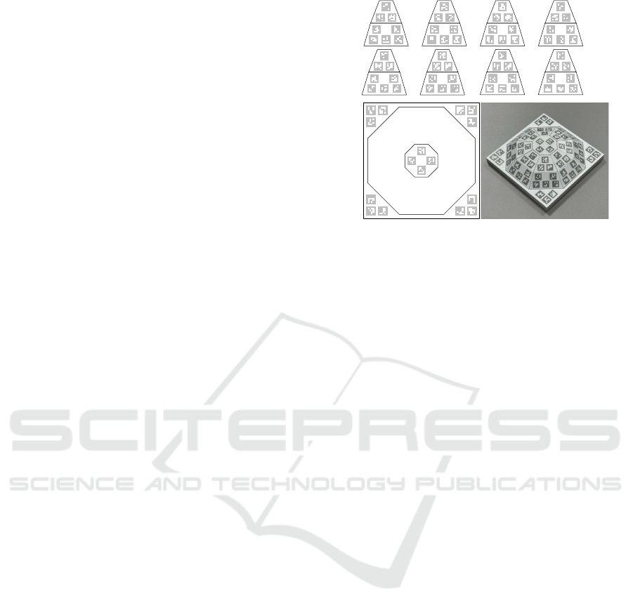
(a)
(b)
Figure 1: Our novel PMP calibration target design. (a) Un-
folded surfaces with unique fiducial markers, which are at-
tached to the 3D model. (b) A fabricated calibration target.
cial markers, such as Aruco markers (Munoz-Salinas,
2012). Each plane is designed to have detectable
markers with predefined local coordinates, and we set
the plane’s coordinate system at the bottom as refer-
ence world coordinates. In this case, optimizing a ro-
tation and translation from the local coordinate sys-
tem to the world coordinate system is required. Con-
sidering the printing resolution of the markers on each
surface, we result in 18 polygons. They are attached
on each face on a 3D structure (Figure 1b). Also, as
we illuminate sinusoidal phase patterns on the target
to get phase maps, we print patterns with middle gray
colors. Its dimensions are 60 × 60 × 12.3 mm. Note
that the shape of the calibration target is not restricted
to a specific form, and the target described in Figure 1
is a possible example that is applicable to our calibra-
tion method described in Section 4.
Target Geometry Model. Our calibration target
consists of independent planar surfaces which have
their own local coordinates. For convenience, let sur-
face index 0 be the reference surface at the bottom.
i.e., the local coordinate system of surface 0 is the
same as the world coordinate system. Each surface
of our target has enough numbers (3 at least and 12 at
most) of Aruco markers. Each marker has a unique ID
to recognize which surface the corners of the marker
lay on.
Given a point X
si
=
x
si
y
si
0
⊺
∈ R
3
be an lo-
cal coordinate of the i-th corner point in surface s, the
corresponding world coordinates are
ˆ
X
w
=
R
s
t
s
0 1
ˆ
X
si
, (1)
where the hat symbol denotes that a point is expressed
in a homogeneous coordinate notation, and R
s
, t
s
are
the rotation/translation from local coordinates of sur-
face s to world coordinates. Then given rotation and
Joint Calibration of Cameras and Projectors for Multiview Phase Measuring Profilometry
81

translation of surface s, we can derive a plane equa-
tion in terms of n
s
, the normal of the surface and c
s
,
the constant of the surface as: n
s
·X
w
+c
s
= 0 , where
n
s
= R
s
0 0 1
⊺
and c
s
= −n
s
· t
s
.
4 NONLINEAR OPTIMIZATION
OF PMP CALIBRATION
Overview. Our nonlinear optimization of calibration
consists of four main steps: First, we detect fidu-
cial markers to obtain plane equations of each sur-
face on the target. The corner points observed by
multiview cameras let us initially calibrate each cam-
era’s parameters as initial. We then illuminate phase-
shift images of different frequencies to compute an
unwrapped phase map for each camera-and-projector
pair. Given the phase maps of all pairs, we compute
the depth values of every pixel in phase maps. Lastly,
by minimizing the sum of distances between the es-
timated depths and the target planes, we optimize the
camera/project parameters iteratively.
4.1 Initial Camera Calibration Using
Target
Camera/Projector Models. We first formulate the
geometry of the camera and the projector by using
the standard pinhole camera model. We also include
a sixth-order radial distortion model for the perspec-
tive camera. The telecentric camera is formulated by
removing the z projection component from the camera
model. The projector is based on the inverse pinhole
camera model. Refer to the supplemental document
for more details.
To calibrate the parameters of a camera in a sin-
gle shot, it is required to capture multiple surfaces
with markers in a single image. Theoretically, at least
three surfaces with different poses should be captured
to build homographies (Zhang, 2000). The optimiza-
tion process consists of two steps. First, a i-th corner
on a surface s is projected to undistorted image coor-
dinate p
csi
(refer to Section 1 in the supplemental doc-
ument). Second, the undistorted pixel index p
undist
csi
is
achieved by the distortion removal process with the
pixel index or detected corner in the image. Then the
loss can be defined as the square of the Euclidean dis-
tance of pixels in the image space between p
csi
and
p
undist
csi
:
L
csi
(p
′
csi
,X
si
) (2)
= ∥p
undist
csi
(p
′
csi
;K
c
,d
c
) − p
csi
(X
si
;R
c
,t
c
,K
c
,R
s
,t
s
)∥
2
2
.
(a) Phase-shifting patterns ( )
1
φ
4
φ
16
φ
64
φ
(b) Reconstructed phase map ( )
(c) Phase maps of four different frequencies (d) Final unwrapped phase map
4
φ
4
φ
Figure 2: (a) Phase-shifting pattern examples with a fre-
quency ( f = 4). (b) The reconstructed phase map. (c) Phase
maps of four different frequencies. (d) Final unwrapped
phase map from camera 1.
Let S
cam
, S
surface
denote a set of cameras and sur-
faces, Θ
cam
, Θ
surface
denote a set of parameter θ
c
=
{K
c
,R
c
,t
c
,d
c
} and θ
s
= {R
s
,t
s
} for every camera
c ∈ S
cam
and surface s ∈ S
surface
, the optimization min-
imizes the sum of losses for every c and corner simul-
taneously.
minimize
Θ
surface
,Θ
cam
∑
c∈S
cam
∑
s∈S
surface
∑
i
L
csi
(p
′
csi
,X
si
). (3)
In the optimization process, the world coordinates of
every Aruco marker’s corner are shared globally. It
prevents a specific camera’s parameters from falling
into local minima because the loss of other cameras
increases when it happens. With the multiview con-
straint, the parameters of every camera and the pose
of every surface converge globally.
4.2 Phase Extraction
A sequence of N sinusoidal structured light images
with a frequency f encodes a phase, which is lin-
early related to the pixel index of a projector in ver-
tical or horizontal direction (Feng et al., 2021). For
k ∈ [0,N − 1], when the n-th structured light image
with frequency f is projected onto an object, the re-
flected light is captured by a camera with the intensity
of I
f k
(u,v) for each pixel u,v. The pixel intensity is
formulated as follows:
I
f k
(u,v) = I
a
(u,v) +I
b
(u,v)cos(φ
f
(u,v) +2πk/N),
(4)
where φ
f
(u,v) ∈ [− f π, f π]. We then easily recon-
struct the phase φ by
φ
f
(u,v) = tan
−1
∑
N−1
k=0
I
f k
(u,v)sin(2πk/N)
∑
N−1
k=0
I
f k
(u,v)cos(2πk/N)
. (5)
We capture images with structured lights of four fre-
quencies: 1, 4, 16, and 64. A sequence of wrapped
VISAPP 2025 - 20th International Conference on Computer Vision Theory and Applications
82
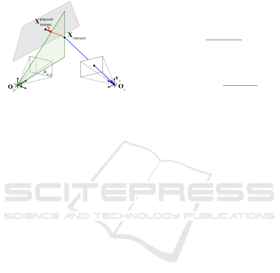
camera
projector
Calibration
target surface
n
x
s
Figure 3: Visualization of our bundle-adjusting calibration.
Once we obtain an unwrapped phase map, we can measure
depth by computing an intersection point X
intersect
with a
plane formed by x
n,p
(green plane) and a camera vector
x
n
(blue arrow). Given X
intersect
, our nonlinear optimiza-
tion updates the camera and the projector’s parameters it-
eratively by minimizing the distance between X
intersect
and
X
projected
intersect
(red line) along the surface normal n
s
of the target
surface s (red arrow).
phase φ
f
(u,v) is unwrapped to obtain ψ(u, v). Note
that we print the fiducial markers with the middle gray
color in order to decode phase shift patterns without
artifacts. See Figure 2 for an example. Refer to the
supplemental document for more details.
Phase Outlier Removal. Since a phase map pro-
duced by a series of images is weak to the noise of
the images, a minor noise occurring to a pixel of a sin-
gle image can bring about serious errors in 3D points.
Therefore, we must filter out the noisy phases from
the phase map to reconstruct the correct shape. Refer
to the supplemental document.
4.3 Nonlinear Optimization
Depth by Intersection. Given a pair of camera pixel
(u
c
,v
c
) and phase (ψ
u
(u
c
,v
c
),ψ
v
(u
c
,v
c
)) achieved
by horizontally and horizontally structured light, we
can obtain the intersection point X
intersect
by com-
puting an intersection point between a phase plane
from the projector and a ray vector from the cam-
era. In Figure 3, x
n,p
(or y
n,p
) can be obtained with
(ψ
u
(u
c
,v
c
),ψ
v
(u
c
,v
c
)) and projector intrinsics. Then,
given the line x = x
n,p
(or y = y
n,p
) on the normalized
projector plane and the projector’s center of projec-
tion (COP) O
p
, we can calculate the normal of phase
plane n
p
(green arrow). Then the phase plane (green
plane) can be expressed as {X : n
p
· (X − O
p
) = 0},
where X is a point in the world coordinates.
And we can express a unit vector of pixel ray from
the camera (blue arrow) as v
c
= x
n
− O
c
, where x
n
is
the point on normalized camera plane gained by pixel
coordinates (u
c
,v
c
), and O
c
is the COP of the camera.
Then, point X can be expressed as {X : X = O
c
+
λv
c
}. Then we can figure out X
intersect
by solving λ,
z
c
= λ =
n
p
· (O
p
− O
c
)
n
p
· v
c
. (6)
Similarly, we can represent point X captured by a
telecentric lens camera as {X : X = x
n
+ λv
c
}, where
v
c
= R
−1
c
0 0 1
⊺
. Then we can solve λ as
z
c
= λ − 1, λ =
n
p
· (O
p
− x
n
)
n
p
· v
c
. (7)
Then the intersection point is X
intersect
= O
c
+ λv
c
with the pinhole camera, and X
intersect
= x
n
+λv
c
with
the telecentric lens camera.
Bundle-Adjusting Optimization. Let S
proj
and
Θ
proj
denote a set of projectors and a set of parame-
ter θ
p
= {K
p
,R
p
,t
p
,d
p
} for every projector p ∈ S
proj
.
For each surface s of our target, we can obtain the
pixel area A(c,s) of the same orientation, where the
marker exists in the camera image c, because each
fiducial marker has a unique ID. Since the pose of a
surface of the target is optimized in Section 4.1, we
can define a loss of bundle adjustment as a distance
between X
intersect
and a surface (red line) along the
surface normal (red arrow):
L
bundle
(c, p,s)
=
∑
(u
c
,v
c
)∈A(c,s)
{n
s
X
intersect
(u
c
,v
c
,ψ
u,p
(u
c
,v
c
),
ψ
v,p
(u
c
,v
c
);θ
c
,θ
p
) + c
s
}
2
. (8)
Since cameras and projectors affect each other, the
overall bundle adjustment process should be per-
formed simultaneously:
minimize
Θ
cam
,Θ
proj
∑
p∈S
proj
∑
c∈S
cam
∑
s∈S
surface
L
bundle
(c, p,s). (9)
Unlike other existing camera-projector calibration
methods using bundle-adjustment approach (Furu-
akwa et al., 2009; Garrido-Jurado et al., 2016; Li
et al., 2019), we introduce an additional condition that
the calibration target consists of planar surfaces and
assume their orientations are known via Equation (3).
Therefore, the objective function has a form of the
sum of point-plane distance errors rather than repro-
jection errors. We have achieved sufficiently accurate
parameters, through our calibration target and bundle-
adjustment approach, to reconstruct microscopic de-
tails of the object without requiring additional uni-
form color illumination as needed in (Li et al., 2019).
Joint Calibration of Cameras and Projectors for Multiview Phase Measuring Profilometry
83

4.4 Reconstruction
Prior to reconstructing 3D point clouds, we measure
a confidence map corresponding to a depth map. A
confidence map is used for two purposes. First, we
can filter out the points with low confidence. Second,
confidence values can be used to refine the 3D shape.
For each D
c
, a depth map achieved from a camera c
is required to calculate the confidence of each pixel.
Given X
c
(u,v), a 3D point obtained from D
c
(u,v) can
be transformed into the camera coordinate of another
camera c
′
:
ˆ
X
c
′
=
x
c
′
y
c
′
z
c
′
1
=
R
c
′
t
c
′
0 1
R
c
t
c
0 1
−1
ˆ
X
c
. (10)
Then the point
ˆ
X
c
′
can be projected to a pixel p
c
′
=
u
′
v
′
⊺
. Finally, in terms of the difference between
the z
c
′
and D
c
′
(u
′
,v
′
), the confidence of the pixel (u, v)
with the camera c is computed as follows
C
c,c
′
(u,v) =
(
1, if V
c
′
(X
c
(u,v)) = 0,
exp{−(z
c
′
− D
′
c
(u
′
,v
′
))
2
}, otherwise,
(11)
where V
c
′
is a visibility term which is 1 if X
c
(u,v)
is visible to c
′
and 0 otherwise. The final confidence
C
c
(u,v) is obtained by
C
c
(u,v) =
∏
c
′
∈S
cam
,c
′
̸=c
C
c,c
′
(u,v). (12)
Then we can get rid of the pixels that C
c
(u,v) < τ
conf
.
After all, a set of total point clouds and corre-
sponding confidences are obtained by spreading out
D
c
and C
c
to the world space for every camera c ∈
S
cam
. Now let S
total,c
(u,v) be a set whose element is
a paired depth d of visible point X
c
in the total point
cloud from a pixel (u,v) of camera c and correspond-
ing confidence weight ω. Then the refined depth map
D
refined
c
is obtained as a weighted sum of depth whose
weight is the confidence as follows:
D
refined
c
(u,v) =
∑
(d,ω)∈S
total,c
(u,v)
ω · d
∑
(d,ω)∈S
total,c
(u,v)
ω
. (13)
5 EXPERIMENTAL RESULTS
Experiment Setup. We build a multiview PMP
setup with five cameras and four projectors. We place
a telecentric-lens camera on top and four ordinary
cameras in four cardinal directions on a metallic sup-
port. On top of each side camera, we install four
projectors illuminating four different frequencies with
Camera 0
Camera 1
Camera 2
Camera 3
Camera 4
Projector 0
Projector 1
Projector 2
Projector 3
Figure 4: Schematic diagram of the cross-section view of
our multiview PMP imaging setup.
four tap phase shifts with π/2 intervals. See Figure 4.
Since we design our target convex for each side of the
target to get as much light from a projector as pos-
sible, we pair a projector with every camera except
for the camera in the opposite direction in the cali-
bration procedure. On the other hand, we pair a pro-
jector only with the top-view camera and the camera
on the same side in the reconstruction procedure to
reduce the risk of noise produced from the shadowed
area of a non-convex object. We have implemented
our optimization with the Adam optimizer in Pytorch,
and rigid body transformations are optimized via Li-
etorch (Teed and Deng, 2021).
5.1 Multiview Reconstruction Results
Now we demonstrate multiview 3D reconstruction re-
sults.
Real-World Object Results. Figure 5 demonstrates
our multiview 3D reconstruction results. From the
leftmost end, we show (a) photographs of objects, (b)
multiview phases from different views, (c) the com-
bined depth, and (d) the final 3D reconstruction re-
sults rendered in different angles. As shown in the
coin object, the microscale geometry of the object is
captured with high accuracy, i.e., the height of the
Queen’s relief is less than 500 µm. The side geom-
etry of the coin is also clearly acquired by the side-
view observation registered by our method with high
accuracy. Moreover, the detailed geometries, such as
letters inscribed in the statue, are well reconstructed
in our method. Other objects’ front and side surfaces,
like dolls, can be scanned with high accuracy. Also,
note that the front surfaces of the object are recon-
structed with multiview phase maps. No artifact at
the front reflects highly accurate registration results
by our calibration method.
Multiview Reconstruction Accuracy. In order to
evaluate the registration accuracy of multiview depth
maps to the final geometry, we compare our multi-
view 3D reconstruction results with 3D geometry ac-
quired by a commercial laser scanner, NextEngine.
To achieve the most detailed and accurate geometry
VISAPP 2025 - 20th International Conference on Computer Vision Theory and Applications
84
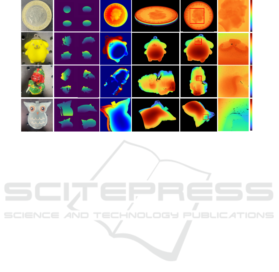
(a) Photograph (b) Multiview phase (c) Combined depth (d) 3D reconstruction rendered in different angles
height (mm)0 4.66height (mm)0 24.28
height (mm)0
25.13
height (mm)0
20.62
Closeup
Figure 5: 3D reconstruction results of real-world objects. (a) Photographs of objects. (b) Multiview phase maps. (c) Combined
depth maps. (d) 3D reconstruction rendered in different views.
from the scanner, we use one-pass scanning results
by the scanner. For a fair comparison, we compare
the one-pass scan results with our multiview recon-
struction results, evaluating Hausdorff’s distance be-
tween the laser-scanned 3D data and the point cloud
reconstructed by our method. Note that the distances
in overlapping areas are significantly low, while high
errors occur only when there is no geometry in the
NextEngine scan results. As shown in Figure 6, our
reconstructed geometry from multiview phase mea-
surements presents a good agreement with geometry
measurement by the commercial scanner. This means
that the system parameters estimated by our nonlinear
optimization using our static target are highly accu-
rate.
Confidence Filtering. Before reconstructing 3D ge-
ometry, it is essential to estimate a confidence map
given a depth map. Since we measure the confidence
of a depth map pixel-by-pixel by comparing depth
maps in the multi-view system, we can mitigate the
risk of reconstructing invalid depths from the wrong
phase input. Given the geometrical relationships be-
tween multiple views, we can measure reliability and
filter them out by evaluating if a point is not supposed
to exist in the depth maps of the other views. As
shown in Figure 7(b), the leg of the knight on the left-
most side of the image produces invalid phase input to
a camera view because its points are not reconstructed
in a consistent place by the camera. It validates that
our confidence-based filter algorithm performs well
in removing unreliable points. Then, other reliable
depth values are combined into the final 3D geometry
as shown in Figure 7(d).
5.2 Camera Intrinsic Compared with
Zhang’s Method
To validate parameters calibrated by our method, we
compare the reprojection errors of our method for
9 × 8 checkerboard corners with standard Zhang’s
method (Zhang, 2000). To do this, we prepare a cali-
bration image set consisting of 15 images of different
checkerboard poses to calibrate Zhang’s method. The
reprojection errors are measured with the same val-
idation image set for both Zhang’s and our method.
Tab. 1 shows the reprojection error results, and Fig. 8
shows the checkerboard images marked with repro-
jected corners of Zhang’s and ours. Since we use a
static target where each surface orientation is fixed
and surface orientation observation locally isolated,
the errors of our method tend to be higher than
Zhang’s. However, we demonstrate that our method
shows errors of less than 1 pixel. The error difference
between the standard method and ours is very simi-
lar even only our method does not require changing
the surface orientation and our method just uses the
single static scene of our target.
5.3 View-Pairwise Consistency Results
In this section, we demonstrate that each depth map
built from a view before the final reconstruction fits
Joint Calibration of Cameras and Projectors for Multiview Phase Measuring Profilometry
85
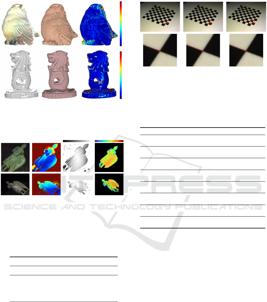
(c) Geometry differences
0.707
0
(a) NextEngine scanner (b) Our method
0 0.866
Hausdorff distance (mm) Hausdorff distance (mm)
Figure 6: Accuracy evaluation of our registration using the
optimized calibration parameters. (a) 3D geometry captured
by a commercial scanner. (b) Our multiview reconstruction
result. (c) Hausdorff’s distance map. Blue means zero error.
(a) Photograph !
(b) Depth map!
(c) Confidence map!
Confidence!0! 1!
(d) Reconstruction result!
height (mm)!0! 4.66!
Figure 7: Our confidence filtering results. (a) Object pho-
tographs from different views. (b) Estimated depth maps
from each view. (c) Confidence maps that we computed
through reprojection. (d) Final 3D reconstruction result ren-
dered from each view.
Table 1: Reprojection errors of the validation sets of images
with standard pinhole camera calibration method and our
method.
Zhang Ours
RMSE MAE RMSE MAE
Cam 0 0.4938 0.1892 0.8543 0.3513
Cam 1 0.4028 0.1590 0.5612 0.2116
Cam 2 0.3416 0.1348 0.4058 0.1570
Cam 3 0.4349 0.1664 0.7204 0.2794
well. The overall process and corresponding middle
results are shown in Fig. 9. It is evidence of accurate
calibration that a point cloud generated from a view
has a consistent shape with respect to the point cloud
from another view without any post-processing, such
as rigid-body registration. The results described in
this section are measured with point clouds before the
final reconstruction sampled with voxels whose diam-
eter is 0.025mm.
(a) Detected! (b) Reprojected (Zhang)! (b) Reprojected (ours)!
Figure 8: The images (top) and their close-ups (bottom).
(a) 9 × 8 checkerboard image marked with detected corners.
(b) Corners reprojected by Zhang’s method. (c) Corners
reprojected by our method.
Table 2: Statistics including mean and standard deviation
(SD) of Hausdorff’s distance between point clouds gener-
ated by four side-views and top view for various real-world
objects.
View 0 View 1 View 2 View 3
Owl
Mean 0.0817 0.1149 0.126 0.1197
SD 0.1077 0.1536 0.1626 0.1489
Pouch
Mean 0.0393 0.0427 0.0493 0.0367
SD 0.0534 0.0689 0.0772 0.0527
Cat
Mean 0.1168 0.0851 0.1024 0.0945
SD 0.1504 0.1129 0.1334 0.1304
Tire
Mean 0.1027 0.0795 0.0961 0.0953
SD 0.1496 0.1228 0.1432 0.1429
Girl statue
Mean 0.0605 0.0565 0.0488 0.0687
SD 0.0826 0.0853 0.0663 0.1028
Canon holder
Mean 0.1091 0.0691 0.1382 0.1043
SD 0.1566 0.1205 0.1643 0.1423
Singapore lion statue
Mean 0.0945 0.0947 0.0906 0.0838
SD 0.1479 0.1416 0.1404 0.1400
Yellow doll
Mean 0.1188 0.1058 0.1825 0.0986
SD 0.1669 0.1515 0.2125 0.1242
Hausdorff Distance. First, we measure Hausdorff’s
distance between point clouds generated from a dif-
ferent view. Since the top-view camera mainly ob-
serves an object, we compare each point cloud gen-
erated from a side-view camera with the point cloud
generated from the top-view camera. Since there must
be a region that is not overlapped, we measure the
mean and variance of Hausdorff’s distances less than
0.5mm to accurately measure the distance between
overlapped regions. Tab. 2 shows the statistical re-
sults for Hausdorff’s distances of the objects in the
paper and supplemental. We can figure out that ev-
ery depth map fits each other with the distance in the
range between 30µm to 200µm. Fig. 10 shows the
point clouds colored by Hausdorff’s distances, we can
figure out that Hausdorff’s distance of a point in the
overlapped region is extremely low.
Iterative Closest Point. Secondly, we measure
the errors between point clouds by registration of a
point cloud from side-view to the point cloud from top
VISAPP 2025 - 20th International Conference on Computer Vision Theory and Applications
86
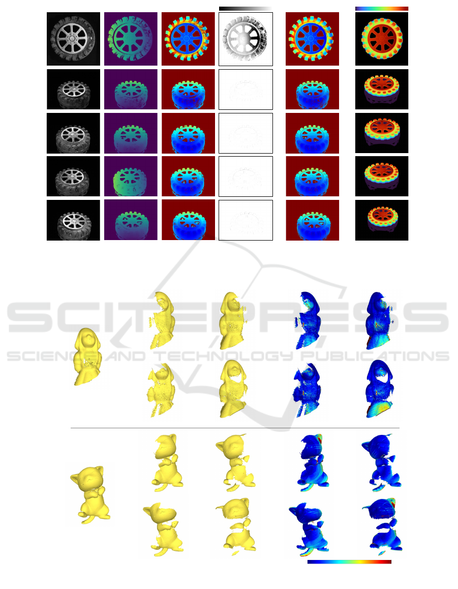
(a) Photograph (c) Depth map
(d) Confidence map
Confidence 0.9 1
(f) Reconstruction result
height (mm) 16.39 23.20
(e) Combined depth map
(b) Phase map
Figure 9: 3D reconstruction results of real-world objects with a top-view (the first row) and 4 side-views (the second to the
fifth row). (a) Photographs of objects. (b) Multiview phase maps. (c) Multiview depth maps. (d) Multiview confidence maps.
(e) Multiview combined depth maps. (f) 3D reconstruction rendered in different views.
(c) Geometry differences(a) Point clouds (top view) (b) Point clouds (side view)
0 0.5 Hausdorff distance (mm)
Figure 10: Point clouds are generated by depth maps of top and side views and their geometry differences. (a) Point clouds
generated by top view. (b) Point clouds generated by side view. (c) Geometry differences measured as Hausdorff’s distance.
Joint Calibration of Cameras and Projectors for Multiview Phase Measuring Profilometry
87

Table 3: Errors of transformations of R and t with various real-world objects.
View 1 View 2 View 3 View 4
E(R) E(t) E(R) E(t) E(R) E(t) E(R) E(t)
Owl 0.0105 0.2491 0.0096 0.1145 0.0077 0.2770 0.0102 0.1077
Pouch 0.0033 0.0870 0.0027 0.1099 0.0012 0.0588 0.0022 0.0465
Cat 0.0143 0.2934 0.0036 0.1316 0.0084 0.1095 0.0124 0.3287
Tire 0.0053 0.1910 0.0019 0.0552 0.0038 0.0918 0.0034 0.1425
Girl statue 0.0054 0.0365 0.0046 0.0695 0.0016 0.1008 0.0094 0.1661
Canon holder 0.0017 0.2710 0.0026 0.2155 0.0014 0.3009 0.0031 0.2427
Singapore lion statue 0.0066 0.2092 0.0033 0.0946 0.0062 0.1669 0.0054 0.0828
Yellow doll 0.0139 0.1937 0.0182 0.3800 0.0157 0.4056 0.0141 0.1515
Mean 0.0008 0.1914 0.0058 0.1463 0.0006 0.1889 0.0075 0.1586
view (Wang and Solomon, 2019). To do this,
given R and t which represent the transform calcu-
lated from Iterative Closest Point algorithm (Chen
and Medioni, 1992), it is obvious that R = I
3
and t = 0
3
where I
3
and 0
3
3 × 3 denote identity
matrix and 3 × 1 zero vector. We define errors of
rotation and translation as E(R) =
∥
R − I
3
∥
F
and
E(t) =
∥
t
∥
2
. Tab. 3 shows the measured error of ICP
transformation from each side-view 1, 2, 3, and 4
to the top-view with objects in the main paper and
supplement. The reason that the value of E(t) is
higher than Hausdorff’s distance described in Tab. 2
is supposed to be due to the small misalignment of
the rotations.
6 CONCLUSION
We have presented a phase-measuring profilometry
calibration method specially designed for multiview
PMP systems. We propose a novel compact, static
calibration target design, which is applicable to exist-
ing PMP instrument heads even with a small room for
calibration. We tackle the overfitting problem of cali-
bration parameters that often occurs in the static cali-
bration of multiview geometry. We resolve this chal-
lenge by devising a multiview-based bundle-adjusting
approach. Our nonlinear optimization method can
acquire explicit calibration parameters not only for
projectors but also for perspective/telecentric cameras
with high accuracy. No physical interaction is re-
quired during the calibration process. We anticipate
that our method makes the multiview PMP calibra-
tion process simpler, and it is beneficial for the 3D
imaging industry as it can achieve high-accuracy reg-
istration of multiview input.
ACKNOWLEDGEMENTS
Min H. Kim acknowledges the Samsung Research
Funding & Incubation Center (SRFC-IT2402-02),
the Korea NRF grant (RS-2024-00357548), the
MSIT/IITP of Korea (RS-2022-00155620, RS-2024-
00398830, 2022-0-00058, and 2017-0-00072), Mi-
crosoft Research Asia, LIG, and Samsung Electron-
ics.
REFERENCES
Cai, Z., Liu, X., Li, A., Tang, Q., Peng, X., and Gao, B. Z.
(2017). Phase-3d mapping method developed from
back-projection stereovision model for fringe projec-
tion profilometry. Optics express, 25(2):1262–1277.
Chen, L., Huayang, L., Xu, Z., and Huan, Z. (2020). Coding
line structured light based on a line-scan camera and
its calibration. Optics Express, 28(17):24799–24812.
Chen, Y. and Medioni, G. (1992). Object modelling by reg-
istration of multiple range images. Image and vision
computing, 10(3):145–155.
Du, H. and Wang, Z. (2007). Three-dimensional shape mea-
surement with an arbitrarily arranged fringe projec-
tion profilometry system. Optics letters, 32(16):2438–
2440.
Feng, S., Zuo, C., Zhang, L., Tao, T., Hu, Y., Yin, W., Qian,
J., and Chen, Q. (2021). Calibration of fringe projec-
tion profilometry: A comparative review. Optics and
Lasers in Engineering, 143:106622.
Feng, Z., Man, D., and Song, Z. (2019). A pattern and
calibration method for single-pattern structured light
system. IEEE Transactions on Instrumentation and
Measurement, 69(6):3037–3048.
Fu, Y., Wang, Y., Wang, W., and Wu, J. (2013). Least-
squares calibration method for fringe projection pro-
filometry with some practical considerations. Optik,
124(19):4041–4045.
Furuakwa, R., Inose, K., and Kawasaki, H. (2009). Multi-
view reconstruction for projector camera systems
based on bundle adjustment. In Proc. IEEE CVPR
Workshops, pages 69–76. IEEE.
Garrido-Jurado, S., Munoz-Salinas, R., Madrid-Cuevas,
F. J., and Marin-Jim
´
enez, M. J. (2016). Simultaneous
reconstruction and calibration for multi-view struc-
tured light scanning. J. Visual Communication and
Image Representation, 39:120–131.
Guo, H., He, H., Yu, Y., and Chen, M. (2005). Least-squares
calibration method for fringe projection profilometry.
Optical Engineering, 44(3):033603.
Guo, W., Wu, Z., Xu, R., Zhang, Q., and Fujigaki, M.
(2019). A fast reconstruction method for three-
VISAPP 2025 - 20th International Conference on Computer Vision Theory and Applications
88

dimensional shape measurement using dual-frequency
grating projection and phase-to-height lookup table.
Optics & Laser Technology, 112:269–277.
Huang, L., Chua, P. S., and Asundi, A. (2010). Least-
squares calibration method for fringe projection pro-
filometry considering camera lens distortion. Applied
optics, 49(9):1539–1548.
Ibrahim, M. T., Gopi, M., and Majumder, A. (2023). Self-
calibrating dynamic projection mapping system for
dynamic, deformable surfaces with jitter correction
and occlusion handling. In IEEE Int. Symp. on Mixed
and Augmented Reality, pages 293–302.
Jiang, C., Lim, B., and Zhang, S. (2018). Three-
dimensional shape measurement using a structured
light system with dual projectors. Applied optics,
57(14):3983–3990.
Juarez-Salazar, R. and Diaz-Ramirez, V. H. (2019). Flexible
camera-projector calibration using superposed color
checkerboards. Optics and Lasers in Engineering,
120:59–65.
Juarez-Salazar, R., Giron, A., Zheng, J., and Diaz-Ramirez,
V. H. (2019). Key concepts for phase-to-coordinate
conversion in fringe projection systems. Applied op-
tics, 58(18):4828–4834.
Lanman, D. and Taubin, G. (2009). Build your own 3d scan-
ner: 3d photography for beginners. In ACM siggraph
2009 courses, pages 1–94.
L
´
eandry, I., Br
`
eque, C., and Valle, V. (2012). Calibration
of a structured-light projection system: development
to large dimension objects. Optics and Lasers in En-
gineering, 50(3):373–379.
Lee, Y. B. and Kim, M. H. (2017). Integrated calibration of
multiview phase-measuring profilometry. Optics and
Lasers in Engineering, 98:118–122.
Li, C., Monno, Y., Hidaka, H., and Okutomi, M. (2019).
Pro-cam ssfm: Projector-camera system for structure
and spectral reflectance from motion. In Proc. IEEE
ICCV, pages 2414–2423.
Li, J.-L., Su, H.-J., and Su, X.-Y. (1997). Two-frequency
grating used in phase-measuring profilometry. Ap-
plied Optics, 36(1):277–280.
Li, W., Li, H., and Zhang, H. (2020). Light plane calibration
and accuracy analysis for multi-line structured light
vision measurement system. Optik, 207:163882.
Li, W., Su, X., and Liu, Z. (2001). Large-scale three-
dimensional object measurement: a practical coordi-
nate mapping and image data-patching method. Ap-
plied Optics, 40(20):3326–3333.
Li, Y., Qian, J., Feng, S., Chen, Q., and Zuo, C. (2022).
Composite fringe projection deep learning profilom-
etry for single-shot absolute 3d shape measurement.
Optics express, 30(3):3424–3442.
Li, Y., Su, X., and Wu, Q. (2006). Accurate phase–height
mapping algorithm for pmp. Journal of Modern Op-
tics, 53(14):1955–1964.
Lin, B., Fu, S., Zhang, C., Wang, F., and Li, Y. (2020).
Optical fringe patterns filtering based on multi-stage
convolution neural network. Optics and Lasers in En-
gineering, 126:105853.
Ma, Q., Cao, Y., Chen, C., Wan, Y., Fu, G., and Wang, Y.
(2018). Intrinsic feature revelation of phase-to-height
mapping in phase measuring profilometry. Optics &
Laser Technology, 108:46–52.
Moreno, D. and Taubin, G. (2012). Simple, accurate, and
robust projector-camera calibration. In 2012 Second
International Conference on 3D Imaging, Modeling,
Processing, Visualization & Transmission, pages 464–
471. IEEE.
Munoz-Salinas, R. (2012). Aruco: a minimal library for
augmented reality applications based on opencv. Uni-
versidad de C
´
ordoba.
Sansoni, G., Carocci, M., and Rodella, R. (2000). Cal-
ibration and performance evaluation of a 3-d imag-
ing sensor based on the projection of structured light.
IEEE Transactions on instrumentation and measure-
ment, 49(3):628–636.
Takeda, M. and Mutoh, K. (1983). Fourier transform pro-
filometry for the automatic measurement of 3-d object
shapes. Applied optics, 22(24):3977–3982.
Teed, Z. and Deng, J. (2021). Tangent space backpropa-
gation for 3d transformation groups. In Proceedings
of the IEEE/CVF Conference on Computer Vision and
Pattern Recognition, pages 10338–10347.
Tehrani, M. A., Gopi, M., and Majumder, A. (2019). Auto-
mated geometric registration for multi-projector dis-
plays on arbitrary 3d shapes using uncalibrated de-
vices. IEEE transactions on visualization and com-
puter graphics, 27(4):2265–2279.
Triggs, B., McLauchlan, P. F., Hartley, R. I., and Fitzgibbon,
A. W. (1999). Bundle adjustment—a modern synthe-
sis. In International workshop on vision algorithms,
pages 298–372. Springer.
Ueda, K., Ikeda, K., Koyama, O., and Yamada, M. (2022).
Absolute phase retrieval of shiny objects using fringe
projection and deep learning with computer-graphics-
based images. Applied Optics, 61(10):2750–2756.
Wang, C. and Pang, Q. (2022). The elimination of errors
caused by shadow in fringe projection profilometry
based on deep learning. Optics and Lasers in Engi-
neering, 159:107203.
Wang, Y. and Solomon, J. M. (2019). Prnet: Self-supervised
learning for partial-to-partial registration. Advances in
neural information processing systems, 32.
Wang, Z., Nguyen, D. A., and Barnes, J. C. (2010). Some
practical considerations in fringe projection profilom-
etry. Optics and Lasers in Engineering, 48(2):218–
225.
Xiao, Y., Cao, Y., and Wu, Y. (2012). Improved algorithm
for phase-to-height mapping in phase measuring pro-
filometry. Applied optics, 51(8):1149–1155.
Zhang, Z. (2000). A flexible new technique for camera cal-
ibration. IEEE Transactions on Pattern Analysis and
Machine Intelligence, 22(11):1330–1334.
Zhang, Z., Ma, H., Zhang, S., Guo, T., Towers, C. E., and
Towers, D. P. (2011). Simple calibration of a phase-
based 3d imaging system based on uneven fringe pro-
jection. Optics letters, 36(5):627–629.
Zhang, Z., Towers, C. E., and Towers, D. P. (2007).
Uneven fringe projection for efficient calibration in
high-resolution 3d shape metrology. Applied Optics,
46(24):6113–6119.
Joint Calibration of Cameras and Projectors for Multiview Phase Measuring Profilometry
89
