Editing Scene Illumination and Material Appearance
of Light-Field Images
Jaemin Cho
1 a
, Dongyoung Choi
1 b
, Dahyun Kang
1 c
, Gun Bang
2 d
and Min H. Kim
1 e
1
School of Computing, KAIST, Daejeon, South Korea
2
Research Department of Media Coding, ETRI, Deajeon, South Korea
Keywords:
Light-Field Image Decomposition, Scene Illumination, Neural Inverse Rendering.
Abstract:
In this paper, we propose a method for editing the scene appearance of light-field images. Our method enables
users to manipulate the illumination and material properties of scenes captured in light-field format, offering
various control over image appearance, including dynamic relighting and material appearance modification,
which leverages our specially designed inverse rendering framework for light-field images. By effectively
separating light fields into appearance parameters—such as diffuse albedo, normal, specular intensity, and
roughness within a multi-plane image domain, we overcome the traditional challenges of light-field imaging
decomposition. These challenges include handling front-parallel views and a limited image count, which
have previously hindered neural inverse rendering networks when applying them to light-field image data.
Our method also approximates environmental illumination using spherical Gaussians, significantly enhancing
the realism of scene reflectance. Furthermore, by differentiating scene illumination into far-bound and near-
bound light environments, our method enables highly realistic editing of scene appearance and illumination,
especially for local illumination effects. This differentiation allows for efficient, real-time relighting rendering
and integrates seamlessly with existing layered light-field rendering frameworks. Our method demonstrates
rendering capabilities from casually captured light-field images.
1 INTRODUCTION
Light-field cameras and devices have revolutionized
image capture and processing in computer vision and
graphics, enabling various applications in novel view
synthesis (Gortler et al., 1996; Choi et al., 2019;
Riegler and Koltun, 2020; Riegler and Koltun, 2021),
scene editing (Jarabo et al., 2014; Mihara et al., 2016),
and augmented reality (Holynski and Kopf, 2018). By
capturing multiple sub-aperture images, they provide
a depth of scene information far beyond what tradi-
tional cameras can offer.
In this paper, we propose a method that allows
for scene editing through our novel decomposition of
light-field images. We target key appearance parame-
ters—diffuse albedo, normals, specular intensity, and
roughness—within the multi-plane image (MPI) do-
a
https://orcid.org/0000-0003-2800-5105
b
https://orcid.org/0000-0003-1896-4038
c
https://orcid.org/0000-0003-2632-0048
d
https://orcid.org/0000-0003-4355-599X
e
https://orcid.org/0000-0002-5078-4005
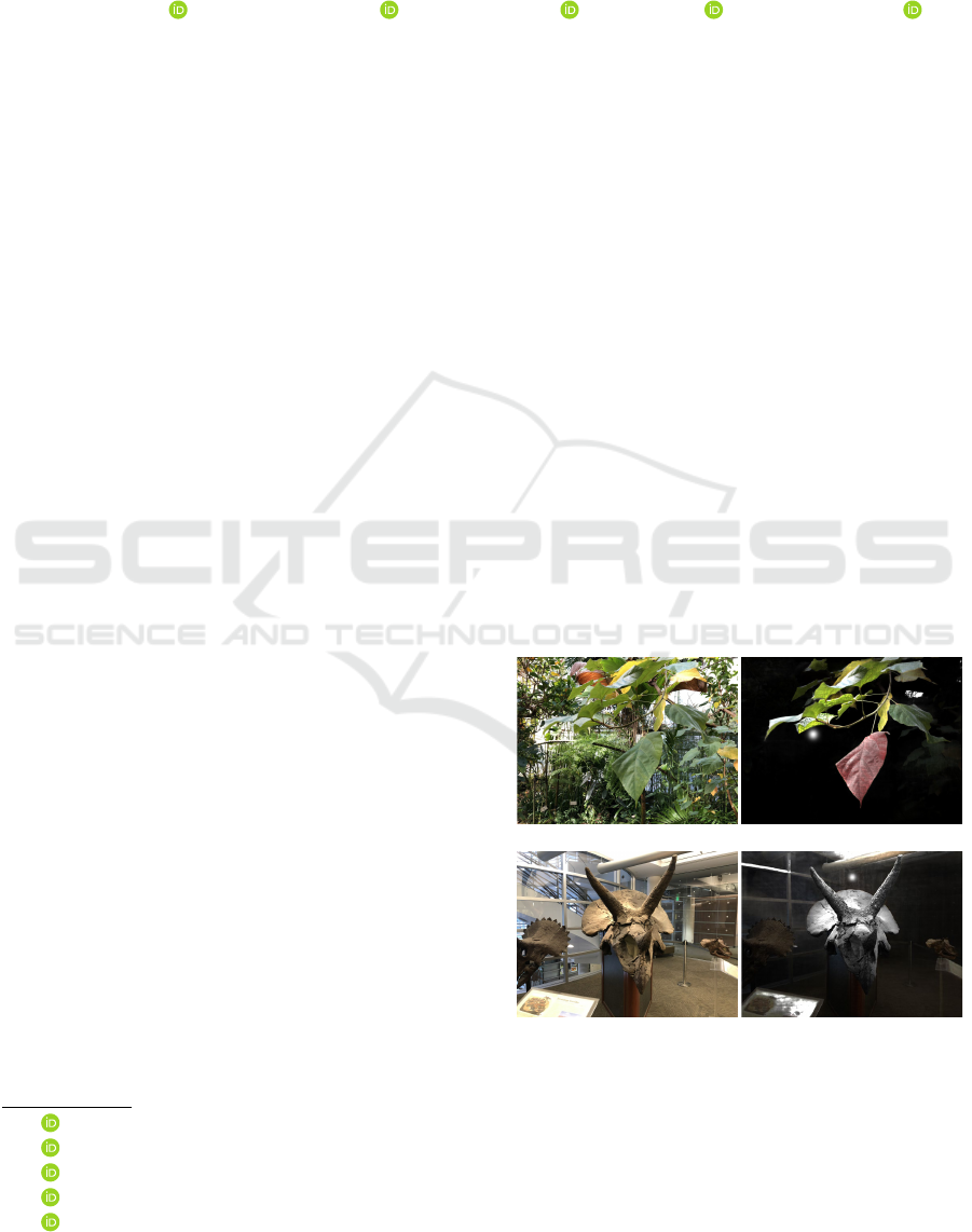
Input Scene editing
Input Scene editing
Figure 1: We present a method to decompose light-field im-
ages into illumination and intrinsic appearance parameters,
enabling realistic relighting and material editing. Refer to
our supplemental video for additional results.
main (Zhou et al., 2018). This technique not only cap-
tures but enhances the realism of environmental illu-
mination, thereby effectively editing material appear-
90
Cho, J., Choi, D., Kang, D., Bang, G. and Kim, M. H.
Editing Scene Illumination and Material Appearance of Light-Field Images.
DOI: 10.5220/0013145500003912
Paper published under CC license (CC BY-NC-ND 4.0)
In Proceedings of the 20th International Joint Conference on Computer Vision, Imaging and Computer Graphics Theory and Applications (VISIGRAPP 2025) - Volume 3: VISAPP, pages
90-101
ISBN: 978-989-758-728-3; ISSN: 2184-4321
Proceedings Copyright © 2025 by SCITEPRESS – Science and Technology Publications, Lda.

ance and scene relighting in casually captured light-
field images as shown in Figure 1.
Despite the richness of the light-field image data,
processing light-field images still presents unique
challenges. Their sub-aperture images typically ex-
hibit front-parallel view directions and a limited count
range, complicating the creation of comprehensive
3D models and the extraction of material appearance
parameters. Furthermore, the conventional methods
for light-field imaging often fall short in depicting
specular reflections accurately due to their reliance on
viewing direction, a limitation that each pixel main-
tains a constant value, regardless of the angle of view
(Flynn et al., 2019; Mildenhall et al., 2019; Zhou
et al., 2018).
Addressing these challenges, we introduce a neu-
ral inverse rendering method especially tailored for
scene-scale light-field inputs within the MPI domain.
Our method employs spherical Gaussian approxima-
tions to segment the light environment into far-bound
and near-bound regions, capturing both global and lo-
cal illumination variations essential for realistic scene
appearance manipulation. The overall process of our
method is visualized in Figure 2. From a given light-
field image, our method decomposes sub-aperture im-
ages into appearance parameters (diffuse albedo, nor-
mal, specular intensity, and roughness) in multi-plane
image space, along with global/local scene illumi-
nation represented as spherical Gaussian functions.
The MPI has 9 channels, with the number next to
each appearance parameter indicating the number of
channels representing that parameter. These decom-
posed elements enable the manipulation of scene ap-
pearance and illumination at a scene-wide scale, not
just for individual objects. This approach not only
boosts rendering efficiency but also ensures seamless
integration with existing light-field rendering archi-
tectures (Flynn et al., 2019; Mildenhall et al., 2019).
By demonstrating practical applications ranging
from relighting to material appearance changes, our
work showcases the versatility and effectiveness of
our method in enhancing the realism and applicability
of light-field imaging for scene editing. Our contribu-
tions are summarized as follows:
• Introducing a scene editing method through a
novel neural inverse rendering for scene-scale
light-field inputs in the MPI domain.
• Enhancing scene realism through global/local il-
lumination estimation using spherical Gaussians.
• Demonstrating practical scene editing applica-
tions, highlighting our method’s versatility in re-
lighting and material appearance modifications.
2 RELATED WORK
Light fields Light fields enable various applica-
tions, including dense depth map capture (Tao et al.,
2013), novel-view image creation (Pozo et al., 2019),
depth of field refocusing (Veeraraghavan et al.,
2007), and 3D content capturing for holographic dis-
plays (Jones et al., 2007). However, the geome-
try information they provide is typically sparser than
that from conventional multiview setups in structure-
from-motion (SfM) or neural rendering. Tradition-
ally, light-field studies have used additional 3D scan-
ning for accurate geometry (Wood et al., 2000;
Lensch et al., 2003). Recent advances include stereo-
imaging methods for dense depth maps (Hedman
et al., 2017; Hedman and Kopf, 2018; Pozo et al.,
2019; Kang et al., 2021) and the use of neural net-
works for novel view synthesis (Srinivasan et al.,
2019; Flynn et al., 2019; Penner and Zhang, 2017;
Choi et al., 2019). Despite these advancements, the
accuracy and view angle variation remain insufficient
for complete inverse rendering. Our work diverges by
focusing on inverse rendering of light fields in MPI
space, decomposing them into scene illumination and
appearance parameters without additional geometry
input.
2.1 Multi-Plane Image
Multi-plane Images (MPI) are used for novel view
synthesis by mapping target image information onto
multiple planes in the reference image’s coordinate
frame via inverse homography (Zhou et al., 2018).
MPIs represent perspective geometry with parallel
planes along the reference camera’s view frustum,
where each plane has RGB and alpha values. In an
MPI with D planes, the transmittance of the d-th plane
(T
d
) and the rendered image color C are defined as:
T
d
= α
d
∏
d−1
i=1
(1 −α
i
). And the color of the rendering
image C is: C =
∑
D
i=1
(c
d
T
d
).
Light-Field Image Decomposition. While light-
field view synthesis has been widely studied (Flynn
et al., 2016; Zhou et al., 2018; Srinivasan et al.,
2019; Flynn et al., 2019; Penner and Zhang, 2017;
Choi et al., 2019; Mildenhall et al., 2019; Broxton
et al., 2020; Wang et al., 2018; Wu et al., 2017;
Wizadwongsa et al., 2021), light-field image decom-
position has seen less progress due to the insuffi-
cient geometry information provided by light fields
alone. Recent advancements have involved mak-
ing specific assumptions, like using dielectric mate-
rials for specular reflection (Tao et al., 2015; Kang
et al., 2021), or formulating joint optimization prob-
Editing Scene Illumination and Material Appearance of Light-Field Images
91

global/local illumination (SGs)
roughness
specular intensity
MPI
diffuse albedo
normal
1
1
1
3
3
transparency
Training images
…
Material editing
Illumination editing
Figure 2: Our method decomposes light-field images into appearance parameters and scene illumination in multi-plane image
space, enabling scene-wide manipulation of appearance and lighting.
lems based on view changes, albedo reflectances, and
material count (Wang et al., 2016; Li et al., 2017;
Ngo et al., 2019). However, these often involve un-
realistic assumptions and focus mainly on depths and
normals, neglecting view-dependent properties. Sub-
sequent methods have adopted physics-based (Kang
et al., 2021), classical graphics (Beigpour et al.,
2018), or perception-based reflectance models (Sulc
et al., 2018) for inverse rendering. Yet, these are typi-
cally formulated on the image plane (Beigpour et al.,
2018) or in the 4D light-field domain (Sulc et al.,
2018), limiting their suitability for efficient and in-
teractive rendering. To address these limitations, our
work proposes a decomposition method in the multi-
plane image space, aiming for more efficient and in-
teractive rendering capabilities.
Neural Inverse Rendering. Neural inverse render-
ing methods such as IRON (Zhang et al., 2022a) and
PS-NeRF (Yang et al., 2022) utilize images captured
under varying lighting conditions for each viewpoint,
with IRON focusing on edge-aware, physics-based
surface rendering and PS-NeRF addressing self-
occlusion in unknown lighting. These approaches
yield high-quality results. Other methods, including
PhySG (Zhang et al., 2021a), NerFactor (Zhang et al.,
2021b), NeRV (Srinivasan et al., 2021), NeILF (Yao
et al., 2022), InvRender (Zhang et al., 2022b), and
TensoIR (Jin et al., 2023), operate under fixed lighting
conditions. While these techniques offer various im-
provements, such as handling self-occlusion and in-
direct illumination, they do not estimate a local illu-
mination profile. VMINER (Fei et al., 2024) mod-
els local illumination as discrete point light sources,
which works well for small, distinct sources. How-
ever, for larger or more complex light sources, this
method becomes computationally expensive. Our
work diverges by estimating both global and local il-
lumination as spherical Gaussians in light fields, fa-
cilitating real-time relighting and natural scene illu-
mination adjustments and maintaining computational
efficiency even with complex lighting setups. Al-
though current state-of-the-art neural inverse render-
ing networks demonstrate high effectiveness in han-
dling single objects, for example, synthetic datasets
used in NeRF (Mildenhall et al., 2020), they struggle
with the unique characteristics of scene-scale light-
field images, such as limited numbers and specific
viewpoint arrangements. Our method addresses these
challenges, enabling effective use in realistic scene
appearance editing and relighting.
3 LIGHT-FIELD
DECOMPOSITION ON MPI
3.1 Preliminaries
Multi-plane image maps target image information
onto multiple planes using inverse homography from
the target to the reference image (Zhou et al., 2018).
MPIs effectively visualize perspective geometry from
forward-facing images. They consist of multiple par-
allel planes within the reference camera’s view frus-
tum, where each plane stores RGB color and alpha
transparency values per pixel. In an MPI with D
planes, RGB color and alpha transparency of the i-
th plane are denoted as c
i
and α
i
, respectively, with
the planes ordered from nearest to farthest from the
viewpoint. The transmittance T
d
of the d-th plane is
given by: T
d
= α
d
∏
d−1
i=1
(1 − α
i
). The rendered image
color C is calculated as: C =
∑
D
i=1
(c
d
T
d
).
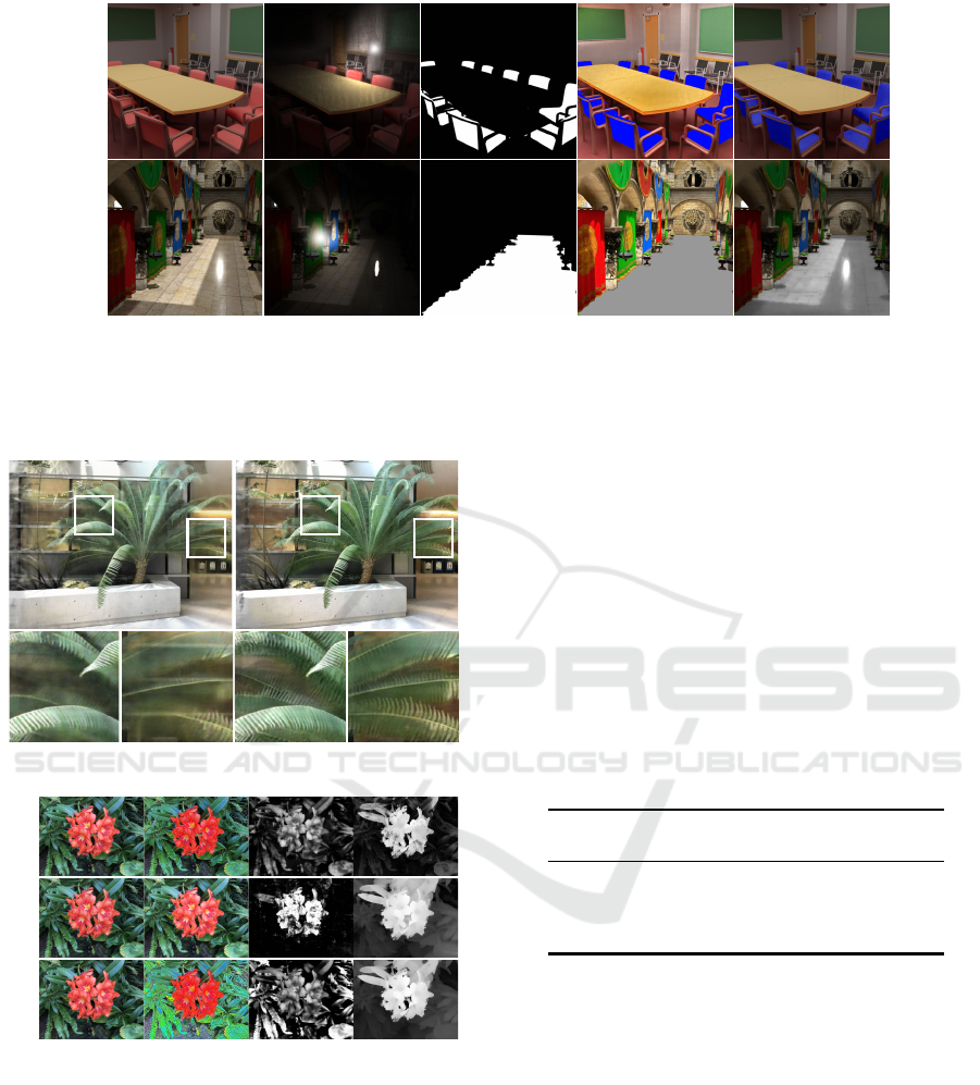
3.2 Geometry Estimation
Our approach begins with geometry estimation, fol-
lowed by material and environment mapping for
physics-based rendering. Given the complexity of
these factors in the final rendering image, we train
VISAPP 2025 - 20th International Conference on Computer Vision Theory and Applications
92

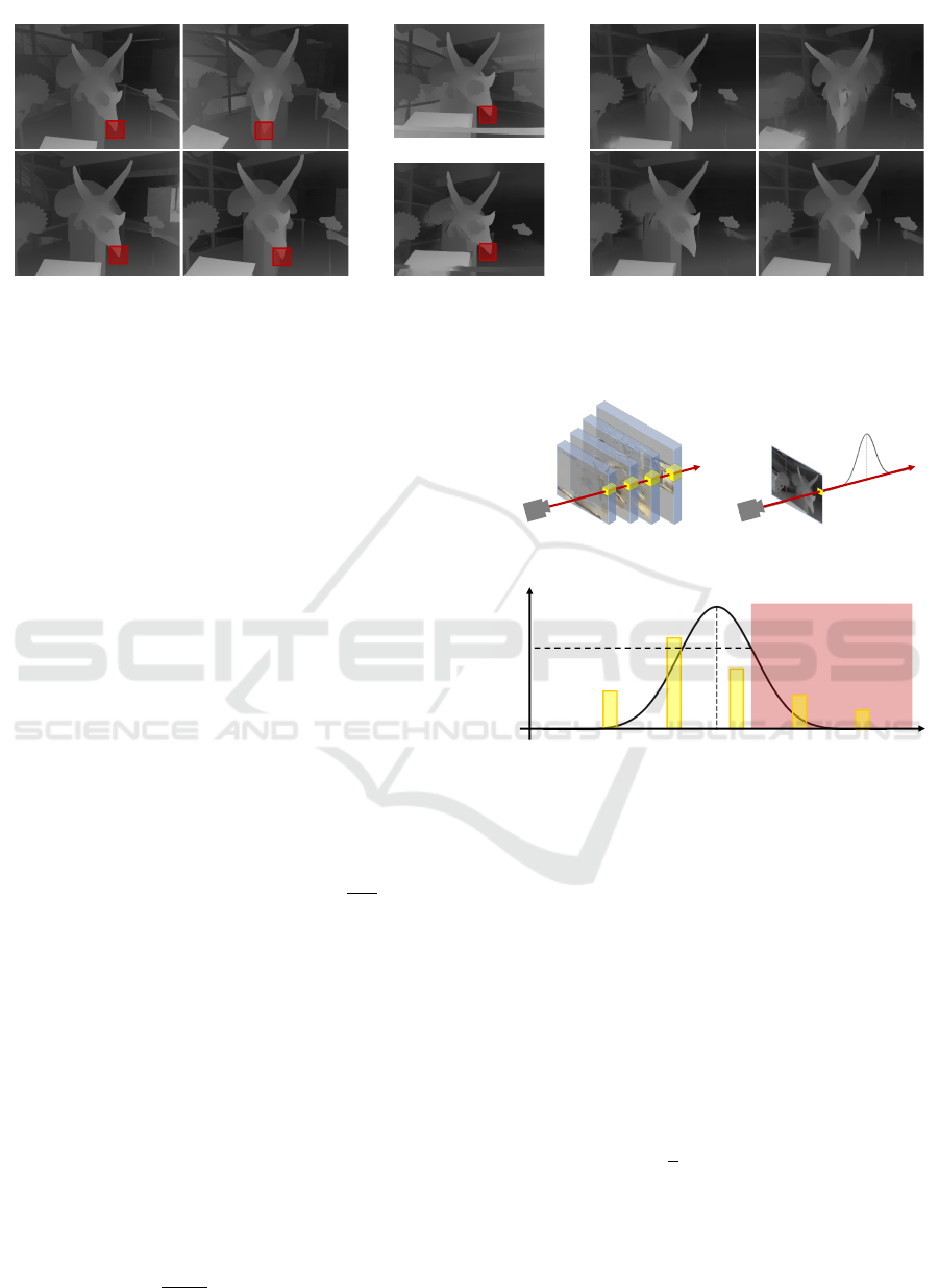
(a) Uncalibrated disparity maps (b) Calibration result
of one disparity map
(c) Calibrated disparity maps
of other views
Before calibration
After calibration
Red boxes indicate the corresponding pixels of 
0

1

2

3

4

0

0
Figure 3: Multiview disparity calibration. (a) Uncalibrated disparity maps and their corresponding pixels to x
0
by optical flow.
(b) Calibration result of one disparity map. (c) Calibrated disparity maps.
these parameters in stages rather than simultaneously.
Initially, we establish a reference geometry, enabling
MPI to train on a geometry. This involves match-
ing pixel correspondences between the target and
sub-camera images using optical flow predicted by
RAFT (Teed and Deng, 2020). We then calculate
the disparity map by minimizing the error in unpro-
jecting matched samples from all camera views into
world space, following Kang et al. (Kang et al., 2021).
To ensure comprehensive geometry training, we com-
pute disparity maps for all image viewpoints, not just
one reference viewpoint. This is crucial as relying on
a disparity map from only one viewpoint may lead
to inadequate training for areas not visible from that
viewpoint.
As shown in Figure 3(a), disparity maps vary with
the viewpoint, leading to blurriness during training.
To correct the value x
0
(the red box in Figure 3(b)), we
find its corresponding pixels in other disparity maps
(the red boxes in Figure 3(a)), and apply the correc-
tion using the following equation: y
0
=
1
β−α
∑
β
i=α
x
i
,
where α and β define the range to eliminate outliers,
with α = [N × 0.10] and β = [N × 0.25]. This range
was determined through experiments:
Finally, we adjust these disparity maps to align
with the reference viewpoint using the extrinsic cam-
era function.
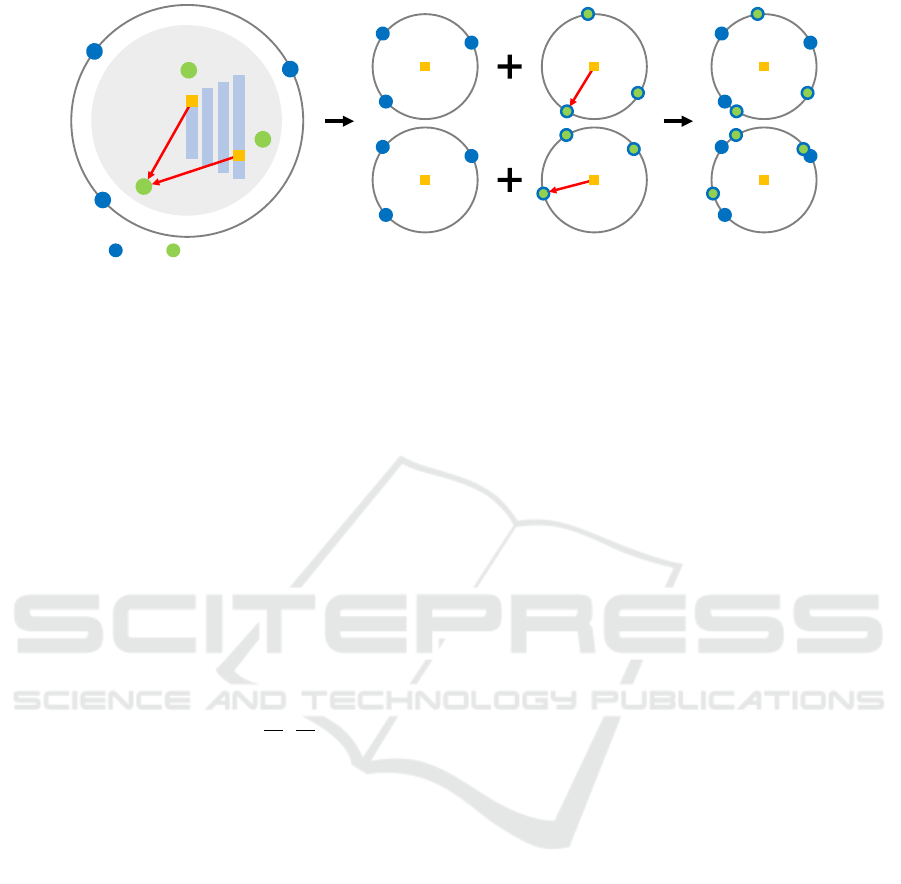
As illustrated in Figure 4, we introduce a loss term
to evaluate the difference between the alpha trans-
parency of the MPI and the reference geometry. In
an MPI with D planes, where the planes are ordered
from nearest to farthest from the viewpoint, we de-
note the i-th plane as p
i
. The alpha transparency of
p
i
is given, and its distance from the reference view-
point is d
i
. For a depth d obtained from the previous
disparity map, we define a 1D Gaussian function f (x)
as: f (x) = exp

−
(x−d)
2
2σ
2

, where σ is the difference
⋯
MPI
Viewpoint
1
p
2
p
3
p
4
p
RAFT disparity map
Viewpoint
d
()fx
(a) Alpha of samples in ray (b) Gaussian of alpha in ray
(c) Difference b/w sampled alpha and Gaussian

Unknown
geometry
0.7
depth
⋯
1
d
2
d
3
d
4
d
D
d
d
()fx
1
α
2
α
3
α
4
α
D
α
Figure 4: Geometry estimation. (a) Utilize the training
viewpoint with corresponding MPI warping and sample α
from the warped MPI. (b) Generate a 1D Gaussian function
of depth, based on the initial disparity map from the training
viewpoint. (c) Illustrate the difference between α
i
and f (x)
along a single ray.
of disparity between planes, and the MPI’s planes are
equidistant in inverse depth space.
Considering that the disparity maps reveal depth
for visible parts but not hidden geometry, our loss
calculation omits differences between alpha trans-
parency and f (x) for non-visible areas. Thus, the loss
between the disparity map and alpha transparency is
defined as:
L
geo
=
1
n
n
∑
i=1
(α
i
− f (d
i
))
2
, (1)
where n is the largest integer fulfilling either (α
n
≤
f (d
n
)) or ( f (d
n
) > 0.7). The geometry of the MPI
was best learned when the threshold value is set to
0.7.
Editing Scene Illumination and Material Appearance of Light-Field Images
93

Disparity maps, generated for all training view-
points, account for geometry invisible from the refer-
ence viewpoint but visible from others. The loss cal-
culation uses the current training image viewpoint, its
disparity map, and the warped MPI for that viewpoint.
However, the original disparity estimation method as-
sumes view-independent imaging, meaning surface
colors do not change with viewing direction. There-
fore, the initially estimated disparity map deviates
from the actual disparity, limiting its use for render-
ing in our model like other methods using known ge-
ometry. To address this, we progressively decrease
the weight of the loss by comparing alpha and dis-
parity maps during training. This approach allows the
model to initially learn approximate geometry quickly
and gradually adjust to correct geometry, particularly
in scenes where the initial disparity map is inaccu-
rate due to view-dependent effects like specular high-
lights.
3.3 Spatially-Varying Reflectance
Estimation
Our model employs physics-based rendering, differ-
ing from traditional MPI models (Mildenhall et al.,
2019; Wizadwongsa et al., 2021) for view synthesis.
It computes the rendering equation using geometry,
material, and light environment. Traditional render-
ing equations involve integrating over hemispheres to
account for all incident light directions. This integra-
tion, often estimated by sampling methods like Monte
Carlo, is computationally expensive and undermines
the primary advantage of traditional MPI, i.e., real-
time rendering.
To avoid this, our approach utilizes a spherical
Gaussian (SG) approximation. This assumes that
the light environment comprises a mixture of SGs,
and the bidirectional reflectance distribution function
(BRDF) is approximated by SGs. An n-dimensional
spherical Gaussian is expressed as: G (ω; ε, λ, µ) =
µe
λ(ω·ε−1)
, where ω ∈ S
2
represents the input, ε ∈ S
2
is the lobe axis, λ ∈ R+ denotes the lobe sharpness,
and µ ∈ R+
n
is the lobe amplitude.
The significant advantage of using SG approxima-
tion in the rendering equation is the elimination of the
sampling process. Since both the integral of an SG
and the inner product of two SGs can be calculated in
closed form, the rendering process becomes substan-
tially more efficient and cost-effective.
In our model, we specifically employ the Cook-
Torrance BRDF for our rendering process. Given
the assumption that the scene comprises dielectric
objects and the training images were captured with
a white balance algorithm, we use a 1-dimensional
Fresnel coefficient F
0
∈ R+, representing specular in-
tensity. Additionally, we utilize 1-dimensional SGs
with mono-color lobe amplitude µ ∈ R+.
The Fresnel function, based on the Schlick
model and approximated by SG, is formulated as:
F (ω
′
i
, h) = F
0
+(1 − F
0
)

1 − cos

θ
′
d

5
, where h is a
half vector between lighting direction ω
i
and viewing
direction ω
o
, ω
′
i
is a vector that reflects ω
o
for sur-
face normal n, and θ
′
d
is the angle between ω
′
i
and h.
Notably, when θ
′
d
is less than 60 degrees, the Fresnel
function F closely resembles the Fresnel coefficient
F
0
. Therefore, we further approximate the Fresnel
function as: F (ω
′
i
, h) ≈ F
0
.
3.4 Global and Local Illumination
Estimation
Our model is designed to estimate geometry, material,
and illumination for scene-scale inputs. This requires
the capability to process both distant light sources,
such as the sun, and nearby light sources. Tradi-
tional methods, which typically use a single environ-
ment map per scene, fall short in representing close,
position-dependent light sources. To address this, we
estimate two distinct types of illumination maps: a
global illumination map for far-bound region and a
local illumination map for near-bound region. The
far-bound region refers to a region where the illumi-
nation is so far from the geometry of the MPI that
it comes in at a constant direction, no matter where
the incident point is located. On the other hand, the
near-bound region is where the illumination is in-situ
light, and its direction changes depending on the posi-
tion of the incident point. Both illumination maps are
formulated as a mixture of spherical Gaussian func-
tions, allowing for a comprehensive representation of
diverse lighting conditions.
Global Illumination. Our global illumination map,
denoted as L
far
, accounts for light sources that are in-
finitely distant. Such light sources provide consistent
direction and intensity regardless of a point’s location
within the scene. We represent this map as a combi-
nation of twelve 1-D spherical Gaussians:
L
far
=
12
∑
k=1
G(ω
i
;ε
k
, λ
k
, µ
k
), (2)
where ε
k
∈ S
2
represents the lobe axis, λ
k
∈ R+ is
the lobe sharpness, and µ
k
∈ R
+
indicates the lobe
amplitude.
Local Illumination. In contrast to global illumina-
tion, local illumination in our model is represented
VISAPP 2025 - 20th International Conference on Computer Vision Theory and Applications
94

SG Light source
MPI
Local Area
1
p
2
p
L
1
p
2
p
Global illumination
Local illumination
(SGs)
Combined illumination
1
p
2
p
(a) (b) (c)
1
p
SG of
L
SG of
L
2
p
Figure 5: Global and local illumination estimation. (a) depicts virtual light sources as green circles and the spherical Gaussians
of the global illumination map as blue circles. (b) shows the SGs of both global and local illumination maps for points p
1
and p
2
. Note that in this figure, both blue and green circles represent SGs. (c) illustrates the combined illumination maps for
points p
1
and p
2
.
using virtual light sources, which vary in direction,
intensity, and sharpness depending on the rendering
location within the scene. Each light source is char-
acterized by its position x
k
∈ R
3
, lobe sharpness λ
k
∈
R+, and amplitude µ
k
∈ R+. These parameters de-
termine the amplitude and sharpness when projected
as spherical Gaussians in the local illumination map.
The map adjusts lobe sharpness and amplitude rela-
tive to each point’s distance from the light sources.
Utilizing 24 virtual light sources per scene, the dis-
tance d
k
from the k-th light source to a point x ∈ R
3
is d
k
=
∥
x − x
k
∥
. The local illumination map L
near
at
this point is represented as:
L
near
=
N
∑
k=1
G

ω
i
;ε
′
k
,
λ
k
d
2
k
,
µ
k
d
2
k

, (3)
where ε
′
k
is the normalized vector of x − x
k
, and N is
the number of virtual light sources. Thus, L
near
com-
prises a mixture of N SGs. And these two local and
global illuminations are integrated into one illumina-
tion map represented by SGs for each pixel, as shown
in Figure 5.
Previous works like NeILF (Yao et al., 2022) and
InvRender (Zhang et al., 2022b) have used point-
specific environment maps, yielding high-quality re-
sults. In contrast, our method differs from InvRender
in that we use virtual light sources to represent point
light in the near-bound region, while InvRender uses
indirect illumination. To represent the results caused
by point light in the near-bound region and indirect
illumination, NeILF uses illumination maps for each
point of the object. However, it cannot distinguish be-
tween global illumination, indirect illumination, and
point light from the learned illumination map. Our
method is specially designed for appearance editing
of light-field images.
This feature is beneficial for relighting tasks, such
as altering the color of a specific light source or re-
moving it entirely. Modifying lights in the light
source group leads to consistent changes in the cor-
responding SGs within the local illumination maps.
Therefore, our model incorporates both a global illu-
mination map and a light source group, projecting the
latter onto the local illumination map for each pixel
in the MPI during rendering and combining it with
the global illumination map for comprehensive scene
illumination.
3.5 Optimization
Our model’s optimization process involves several
loss functions, including the geometric consistency
loss L
geo
from Equation (1). We employ a total varia-
tion of diffuse albedo to promote its local smoothness.
The reconstruction loss is formulated as follows:
L
rec
= α


I
gt
− I


2
2
+ β


∇I
gt
− ∇I


1
, (4)
where I represents the image synthesized by our
model, and I
gt
is the ground truth image.
The transparency loss originates from Neural vol-
ume (Lombardi et al., 2019)’s regularization term that
causes the transparency value of MPI to converge to 0
or 1, defined as follows:
L
tran
= σ(1 − σ) , (5)
where σ is the transparency.
The total loss function, combining these elements,
is defined as:
L
total
= κ(L
rec
+ γTV (ρ)) + ω

L
geo
+ 2L
tran

, (6)
where ρ is the diffuse albedo, and α, β, and γ are
weights balancing the loss terms, set to α = 2, β =
0.5, and γ = 0.03. Weights ω and κ also play a
role, but they are adjusted over epochs. Specifi-
cally, ω decreases and κ increases with the number
Editing Scene Illumination and Material Appearance of Light-Field Images
95

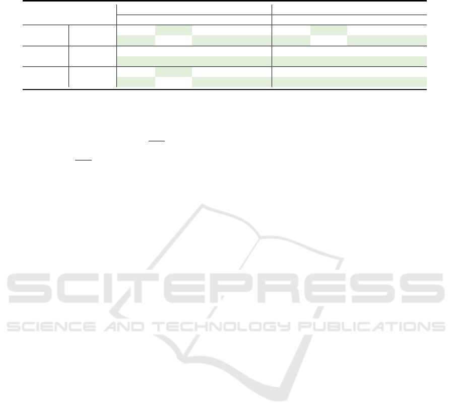
Table 1: Quantitative comparison of average scores for inverse rendering results for the rendering dataset (McGuire, 2017)
obtained with IBL-NeRF (Choi et al., 2023). Green highlights indicate best accuracy.
Conference Sponza
PSNR ↑ SSIM ↑ LPIPS ↓ RMSE ↓ PSNR ↑ SSIM ↑ LPIPS ↓ RMSE ↓
IBL-NeRF 11.97 0.7143 0.3577 0.0635 13.44 0.6151 0.4187 0.0453
Diffuse
Ours 13.87 0.6930 0.3409 0.0410 15.43 0.5645 0.3210 0.0287
IBL-NeRF 8.36 0.1599 0.9236 0.1459 8.62 0.1571 0.7835 0.1375
Normal
Ours 12.47 0.2961 0.7576 0.0567 11.77 0.2897 0.6645 0.0665
IBL-NeRF 38.06 0.9871 0.1771 0.00016 29.67 0.9155 0.2830 0.00109
Rendering
Ours 38.36 0.9747 0.1711 0.00015 32.81 0.9353 0.1032 0.00057
of epochs, reducing the influence of L
geo
and enhanc-
ing the impact of other loss terms as learning pro-
gresses. The values for ω and κ are determined as
follows: ω = min

0.5, 0.05 + 1.1
−
e−900
50

, and κ =
min

1, 0.01 + 1.1
e−801
10

, where e denotes the num-
ber of epochs.
4 EXPERIMENTAL RESULTS
Implementation Details. Our method utilizes a
multilayer perceptron (MLP) for regressing pixel co-
ordinates, a strategy chosen to minimize noise in the
MPI. This MLP, taking pixel coordinates (x, y) from
the d-th plane as input p, predicts alpha transparency
(α) and material information for each pixel. Key
to our approach is the explicit learning of spherical
Gaussians (SGs) and light sources for light fields,
which represent the light environment. This includes
learning parameters like lobe, amplitude, and sharp-
ness. For MPI implementation, we use 192 multi-
plane images, uniformly spaced in disparity space (in-
verse depth). The disparity range for the closest and
furthest MPI from the viewpoint is determined dur-
ing image calibration using SfM (SfM) (Sch
¨
onberger
and Frahm, 2016). In our MLP configuration, the
pixel position (x, y, d) is crucial for predicting pixel-
specific parameters (α, material). Positional encod-
ing (Mildenhall et al., 2020) is applied to the pixel
locations. This results in x and y being encoded into
20 dimensions and d into 16 dimensions, enhancing
the model’s ability to capture fine details in the MPI.
Instead of using an MLP, albedo, global illumination
(SGs), and local illumination (virtual light sources)
are learned explicitly. A vanilla MLP with 6 layers
takes 56 dimensions as input and produces 3 dimen-
sions of output.
4.1 Quantitative Evaluation
Existing neural inverse rendering methods typically
require a large number of inward-looking pho-
tographs for a target object and often struggle with a
limited set of front-parallel light-field images. Among
these methods, IBL-NeRF (Choi et al., 2023) stands
out as it tackles scene-scale inverse rendering prob-
lems akin to our approach.
We use several light-field datasets, which are cap-
tured by large-baseline camera arrays in a structured
and unstructured manner. We then use COLMAP
to estimate the camera parameters. For the real im-
age dataset, we use a real forward-facing light field
dataset (Mildenhall et al., 2019), which consists of
images captured by handheld smartphones. Each
scene has 20 to 62 images, with a resolution of 3982×
2986, which we reduce to a resolution of 1080 × 720
in our method. The synthetic validation rendering
dataset uses the CONFERENCE and SPONZA model-
ing files from a 3D graphics model website (McGuire,
2017) and is rendered as 512 × 512 resolution images
from 49 viewpoints. To assess the effectiveness of our
method, we conducted a comparative analysis with
IBL-NeRF using this rendering dataset.
As shown in Figure 6, the estimated normals of
IBL-NeRF show that the boundaries of objects in the
scene are not clear and mixed, likely due to the limited
number of light-field images available for input.
In contrast, our method demonstrates the capabil-
ity to efficiently decompose light fields into diffuse
albedo, normals, and roughness for each pixel, using
an equivalent number of input images, thus achieving
more accurate and detailed results. Moreover, our ap-
proach excels in learning scene geometry from light
field datasets and consistently estimates uniform ma-
terial properties for each object within the scene. The
comparative results, as presented in Table 1, show
that our method surpasses IBL-NeRF in several key
aspects, including diffuse albedo, normal, roughness,
and overall rendering quality.
4.2 Scene Editing Results
Our inverse rendering method was applied to a real
forward-facing dataset (Mildenhall et al., 2019), con-
sisting of scenes captured from 20 to 30 nearly iden-
VISAPP 2025 - 20th International Conference on Computer Vision Theory and Applications
96

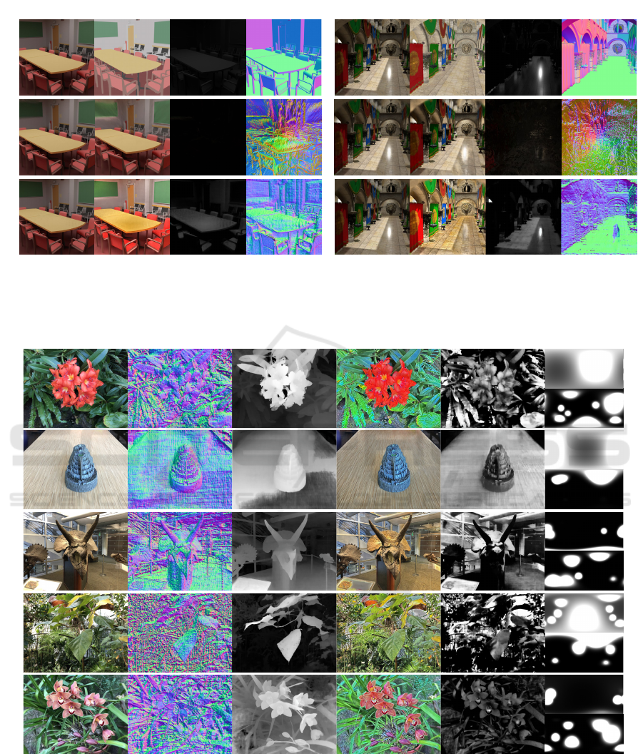
Rendering Diffuse Specular Normal
(b) Sponza
Rendering Diffuse Specular Normal
IBL-NeRFOurs
GT
(a) Conference
Figure 6: Compared to IBL-NeRF (Choi et al., 2023), which struggles with normal estimation due to limited input light-field
images, our method effectively decomposes light fields into normal and material properties, yielding better results. Refer to
Table 1 for quantitative evaluation.
SpecularDiffuseNormal DisparityPhotograph Illumination
Flower
GlobalLocal
Fortress
GlobalLocal
Horns
GlobalLocal
Leaves
GlobalLocal
Orchids
GlobalLocal
GlobalLocalGlobalLocalGlobalLocalGlobalLocalGlobalLocal
Figure 7: Decomposition results by our method with real light-field photographs (Mildenhall et al., 2019). Our method
decomposes input light fields into normal, disparity, and material appearance parameters and the global/local illumination
profiles of the scene as well. This allows us to edit these parameters naturally (as shown in Figure 8).
tical directions. Figure 7 presents the normals, dis-
parity, diffuse albedo, specular intensity, roughness,
and both global and local illumination as estimated
by our method. Despite the limited number of in-
put sub-aperture images, our approach successfully
decomposes the scene’s geometry, normals, and ap-
pearance parameters. The accurate estimation of sur-
face normals contributes to a clear separation of dif-
Editing Scene Illumination and Material Appearance of Light-Field Images
97

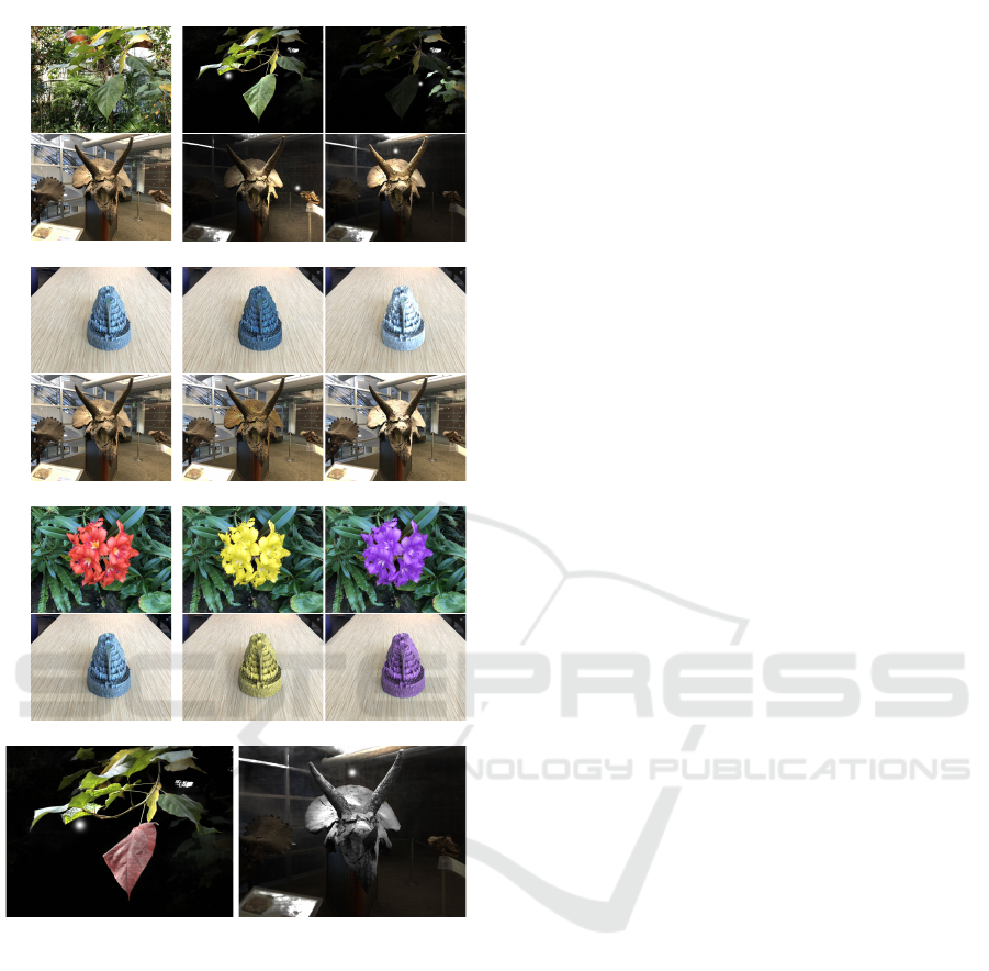
Input Roughness editing
Horns Fortress
Input Albedo editing
Fortress Flower
Input Illumination editing
Horns Leaves
HornsLeaves
Material and illumination editing
Figure 8: Our method enables real-time scene editing. This
allows dynamic changes to lighting and object appearance,
including color and roughness. Refer to the supplemental
video for real-time relighting demonstrations.
fuse albedo from specular intensity, resulting in lo-
cally smooth, shading-free appearances of intrinsic
albedo. The illumination profiles effectively cap-
ture the smooth/sharp and directional qualities of the
scene’s lighting.
Figures 8 and 9 show scene editing results,
demonstrating how changes in material properties and
scene illumination can be effectively implemented.
Our method enables the rendering of realistic images,
even when the albedo and roughness of particular ob-
jects are modified. Furthermore, by substituting the
estimated global and local illuminations with a single
virtual light source, we achieve renderings that accu-
rately represent the altered illumination conditions in
relation to the scene’s surfaces. This not only val-
idates the potential for detailed illumination editing
but also underscores our method’s proficiency in iden-
tifying and integrating internal light sources as part of
the local illumination.
4.3 Ablation Study
Geometry Loss and Local Illumination. Geome-
try loss and local illumination are crucial elements
of our inverse rendering method. We typically use
12 SGs for global illumination and 24 virtual light
sources for local illumination. To assess the impact of
these components, we conduct a comparative study
where we omit local illumination and instead utilize
36 SGs solely for global illumination. As shown in
Figure 10, omitting geometry loss led to inaccura-
cies in complex scenes. Specifically, some objects
that were challenging to model geometrically were
rendered as translucent, erroneously revealing objects
behind them. Additionally, relying solely on global
illumination proved insufficient for accurately repre-
senting scene illumination, resulting in incorrect in-
verse rendering outcomes. These findings underscore
the importance of both geometry loss and local illu-
mination in achieving effective inverse rendering in
complex scenes.
Impact of the Number of SGs. The detail level
in our illumination map is directly influenced by the
number of spherical Gaussians: more SGs lead to a
more detailed representation. However, this bene-
fit comes at the cost of increased computational de-
mands. To find the ideal balance between detail and
efficiency, we conducted training on a real forward-
facing dataset (Mildenhall et al., 2019). The global
illumination does not need high-frequency patterns,
so it can be represented with 12 SGs. Thus, we exper-
imented with increasing the number of virtual light
sources. Note that the number of virtual light sources
influencing local illumination maps corresponds to
the number of SGs in these maps. The view synthesis
quality in our experiments is gauged by images syn-
thesized by the MLP, and the rendering time is mea-
sured from the moment MLP outputs are converted to
MPI format.
Table 2 details the rendering speed performance
across various counts of virtual light sources. We
compare the quality and speed of view synthesis
while increasing the number of virtual light sources
from 12 to 48 with fixed number of SGs represent-
ing global illumination. Using real forward-facing
dataset scenes at a resolution of 1080×720, our model
VISAPP 2025 - 20th International Conference on Computer Vision Theory and Applications
98

(e) Rendering result
with edited albedo
(d) Edited albedo map(c) Object mask(b) Relighting result
Sponza
Conference
(a) Input light fields
Figure 9: Additional scene editing results. (a) Input images for inverse rendering. (b) Rendered images with edited illumi-
nation. (c) Object mask of input images. (d) Albedo images with the albedo of specific objects edited. (e) Rendered images
with edited albedo.
w/ geometry lossw/o geometry loss
(a) View synthesis result wo/w geometry loss
Photograph Diffuse Specular Disparity
w/o
geometry loss
w/o local
illumination
ours
(b) Inverse rendering result
wo/w geometry loss and local illumination
Figure 10: Ablation study. (a) Impact of the geometry loss
in terms of image quality. (b) Impact of geometry loss and
local illumination estimation for inverse rendering results.
achieves a rendering speed of 29 frames per second on
an NVIDIA GeForce RTX 3090. This performance,
while not matching the state-of-the-art method NeX,
is notable considering the additional complexity of
our model, which includes physics-based rendering
and BRDF calculations. As shown in Table 2, quality
scores improve as the number of virtual light sources
increases, yet the improvement plateaus beyond 24
sources. Beyond this number, rendering speed de-
creases significantly. This trend is likely due to the
relatively simple lighting conditions in the real scenes
of our dataset, as opposed to more complex virtual
illumination settings. Therefore, to optimize the bal-
ance between rendering quality and speed efficiency,
we set the number of virtual light sources in our
model to 24 and the spherical Gaussians in the global
illumination map to 12.
Table 2: Ablation study. Average score and rendering speed
comparison according to the number of SGs for the real
forward-facing dataset (Mildenhall et al., 2019). The bold
numbers indicate our choice for experiments.
# of SGs
(global+virtual)
PSNR↑ SSIM↑ LPIPS↓ FPS
24 (12+12) 23.92 0.848 0.270 45
36 (12+24) 24.14 0.857 0.258 29
48 (12+36) 24.19 0.856 0.254 21
60 (12+48) 24.21 0.858 0.255 16
5 DISCUSSION AND
CONCLUSIONS
We have presented a neural inverse rendering method
specifically designed for editing the scene-scale ap-
pearance of light-field images, incorporating elements
of physics-based rendering. This approach effec-
tively learns scene material information and lighting
environments, enabling diverse scene editing tasks
like relighting and altering material appearances with
high fidelity. We represent geometric information as
an MPI, training material data for each scene point,
which is suitable for real-time neural rendering ap-
plications and ensures compatibility with traditional
Editing Scene Illumination and Material Appearance of Light-Field Images
99

MPI architectures. Additionally, our method uniquely
categorizes the lighting environment into far-bound
and near-bound regions, adeptly handling both global
and local illumination of real scenes.
As limitations, our method primarily focuses on
manipulating light intensity, orientation, or hue and
does not alter light relative location of point illumina-
tions. While employing a limited number of spheri-
cal Gaussians effectively captures specular highlights,
it can occasionally encounter challenges in accu-
rately representing more complex specular phenom-
ena, such as mirror reflections.
Also, we acknowledge the presence of checker-
board artifacts in the normal maps and black dots in
the relighting results, which were noted in the sup-
plementary video and figures. These artifacts are a
consequence of the discrete structure of the MPI rep-
resentation with a given spatial resolution. Setting up
a higher spatial resolution for MPI representation can
mitigate these issues.
ACKNOWLEDGEMENTS
Min H. Kim acknowledges the Samsung Research
Funding & Incubation Center (SRFC-IT2402-02),
the Korea NRF grant (RS-2024-00357548), the
MSIT/IITP of Korea (RS-2022-00155620, RS-2024-
00398830, 2022-0-00058, and 2017-0-00072), Mi-
crosoft Research Asia, LIG, and Samsung Electron-
ics.
REFERENCES
Beigpour, S., Shekhar, S., Mansouryar, M., Myszkowski,
K., and Seidel, H.-P. (2018). Light-Field appearance
editing based on intrinsic decomposition. Journal of
Perceptual Imaging, 1(1):010502–1–010502–1.
Broxton, M., Flynn, J., Overbeck, R., Erickson, D., Hed-
man, P., Duvall, M., Dourgarian, J., Busch, J.,
Whalen, M., and Debevec, P. (2020). Immersive light
field video with a layered mesh representation. ACM
Transactions on Graphics (TOG), 39(4):86–1.
Choi, C., Kim, J., and Kim, Y. M. (2023). IBL-NeRF:
Image-based lighting formulation of neural radiance
fields. In CGF, volume 42, page e14929. Wiley On-
line Library.
Choi, I., Gallo, O., Troccoli, A., Kim, M. H., and Kautz,
J. (2019). Extreme view synthesis. In Proc. the
IEEE/CVF ICCV, pages 7781–7790.
Fei, F., Tang, J., Tan, P., and Shi, B. (2024). VMINer:
Versatile multi-view inverse rendering with near-and
far-field light sources. In Proc. the IEEE/CVF CVPR,
pages 11800–11809.
Flynn, J., Broxton, M., Debevec, P., DuVall, M., Fyffe,
G., Overbeck, R., Snavely, N., and Tucker, R. (2019).
Deepview: View synthesis with learned gradient de-
scent. In Proc. the IEEE/CVF CVPR, pages 2367–
2376.
Flynn, J., Neulander, I., Philbin, J., and Snavely, N. (2016).
Deepstereo: Learning to predict new views from the
world’s imagery. In Proc. the IEEE/CVF CVPR, pages
5515–5524.
Gortler, S. J., Grzeszczuk, R., Szeliski, R., and Cohen, M. F.
(1996). The Lumigraph. In Proc. the 23rd annual con-
ference on Computer graphics and interactive tech-
niques, pages 43–54.
Hedman, P., Alsisan, S., Szeliski, R., and Kopf, J. (2017).
Casual 3d photography. ACM Transactions on Graph-
ics (TOG), 36(6):1–15.
Hedman, P. and Kopf, J. (2018). Instant 3d photography.
ACM Transactions on Graphics (TOG), 37(4):1–12.
Holynski, A. and Kopf, J. (2018). Fast depth densification
for occlusion-aware augmented reality. ACM Trans-
actions on Graphics (ToG), 37(6):1–11.
Jarabo, A., Masia, B., Bousseau, A., Pellacini, F., and
Gutierrez, D. (2014). How do people edit light fields?
ACM Transactions on Graphics (SIGGRAPH), 33(4).
Jin, H., Liu, I., Xu, P., Zhang, X., Han, S., Bi, S., Zhou, X.,
Xu, Z., and Su, H. (2023). TensoIR: Tensorial inverse
rendering. In Proc. the IEEE/CVF CVPR.
Jones, A., McDowall, I., Yamada, H., Bolas, M., and De-
bevec, P. (2007). Rendering for an interactive 360
light field display. In ACM SIGGRAPH 2007 papers,
pages 40–es.
Kang, D., Jeon, D. S., Kim, H., Jang, H., and Kim, M. H.
(2021). View-dependent scene appearance synthesis
using inverse rendering from light fields. In Proc. the
IEEE ICCP, pages 1–12. IEEE.
Lensch, H. P., Kautz, J., Goesele, M., Heidrich, W., and
Seidel, H.-P. (2003). Image-based reconstruction of
spatial appearance and geometric detail. ACM Trans-
actions on Graphics (TOG), 22(2):234–257.
Li, Z., Xu, Z., Ramamoorthi, R., and Chandraker, M.
(2017). Robust energy minimization for brdf-invariant
shape from light fields. In Proc. the IEEE/CVF CVPR,
pages 5571–5579.
Lombardi, S., Simon, T., Saragih, J., Schwartz, G.,
Lehrmann, A., and Sheikh, Y. (2019). Neural vol-
umes: Learning dynamic renderable volumes from
images. ACM Transactions on Graphics (TOG),
38(4):65:1–65:14.
McGuire, M. (2017). Computer graphics archive. https:
//casual-effects.com/data.
Mihara, H., Funatomi, T., Tanaka, K., Kubo, H.,
Mukaigawa, Y., and Nagahara, H. (2016). 4d light
field segmentation with spatial and angular consisten-
cies. In Proc. the ICCP.
Mildenhall, B., Srinivasan, P. P., Ortiz-Cayon, R., Kalantari,
N. K., Ramamoorthi, R., Ng, R., and Kar, A. (2019).
Local light field fusion: Practical view synthesis with
prescriptive sampling guidelines. ACM Transactions
on Graphics (TOG), 38(4):1–14.
VISAPP 2025 - 20th International Conference on Computer Vision Theory and Applications
100

Mildenhall, B., Srinivasan, P. P., Tancik, M., Barron, J. T.,
Ramamoorthi, R., and Ng, R. (2020). NeRF: Repre-
senting scenes as neural radiance fields for view syn-
thesis. In Proc. the ECCV.
Ngo, T.-T., Nagahara, H., Nishino, K., Taniguchi, R.-i., and
Yagi, Y. (2019). Reflectance and shape estimation
with a light field camera under natural illumination.
IJCV, 127(11-12):1707–1722.
Penner, E. and Zhang, L. (2017). Soft 3D reconstruction
for view synthesis. ACM Transactions on Graphics
(TOG), 36(6):1–11.
Pozo, A. P., Toksvig, M., Schrager, T. F., Hsu, J., Mathur,
U., Sorkine-Hornung, A., Szeliski, R., and Cabral, B.
(2019). An integrated 6DoF video camera and sys-
tem design. ACM Transactions on Graphics (TOG),
38(6):1–16.
Riegler, G. and Koltun, V. (2020). Free view synthesis. In
Proc. the ECCV, pages 623–640. Springer.
Riegler, G. and Koltun, V. (2021). Stable view synthesis. In
Proc. the IEEE/CVF CVPR, pages 12216–12225.
Sch
¨
onberger, J. L. and Frahm, J.-M. (2016). Structure-
from-motion revisited. In Proc. the IEEE/CVF CVPR.
Srinivasan, P. P., Deng, B., Zhang, X., Tancik, M., Milden-
hall, B., and Barron, J. T. (2021). NeRV: Neural re-
flectance and visibility fields for relighting and view
synthesis. In Proc. the IEEE/CVF CVPR, pages 7495–
7504.
Srinivasan, P. P., Tucker, R., Barron, J. T., Ramamoorthi, R.,
Ng, R., and Snavely, N. (2019). Pushing the bound-
aries of view extrapolation with multiplane images. In
Proc. the IEEE/CVF CVPR, pages 175–184.
Sulc, A., Johannsen, O., and Goldluecke, B. (2018). In-
verse lightfield rendering for shape, reflection and nat-
ural illumination. In Energy Minimization Methods
in CVPR: 11th International Conference, EMMCVPR
2017, Venice, Italy, October 30–November 1, 2017,
Revised Selected Papers 11, pages 372–388. Springer.
Tao, M. W., Hadap, S., Malik, J., and Ramamoorthi, R.
(2013). Depth from combining defocus and corre-
spondence using light-field cameras. In Proc. the
IEEE/CVF CVPR, pages 673–680.
Tao, M. W., Su, J.-C., Wang, T.-C., Malik, J., and Ra-
mamoorthi, R. (2015). Depth estimation and specu-
lar removal for glossy surfaces using point and line
consistency with light-field cameras. IEEE transac-
tions on pattern analysis and machine intelligence,
38(6):1155–1169.
Teed, Z. and Deng, J. (2020). RAFT: Recurrent all-pairs
field transforms for optical flow. In Proc. the ECCV.
Veeraraghavan, A., Raskar, R., Agrawal, A., Mohan, A.,
and Tumblin, J. (2007). Dappled photography: Mask
enhanced cameras for heterodyned light fields and
coded aperture refocusing. ACM Transactions on
Graphics (TOG), 26(3):69.
Wang, T.-C., Chandraker, M., Efros, A. A., and Ramamoor-
thi, R. (2016). SVBRDF-invariant shape and re-
flectance estimation from light-field cameras. In Proc.
the IEEE/CVF CVPR, pages 5451–5459.
Wang, Y., Liu, F., Wang, Z., Hou, G., Sun, Z., and Tan,
T. (2018). End-to-end view synthesis for light field
imaging with pseudo 4DCNN. In Proc. the ECCV,
pages 333–348.
Wizadwongsa, S., Phongthawee, P., Yenphraphai, J., and
Suwajanakorn, S. (2021). NeX: Real-time view syn-
thesis with neural basis expansion. In Proc. the
IEEE/CVF CVPR, pages 8534–8543.
Wood, D. N., Azuma, D. I., Aldinger, K., Curless, B.,
Duchamp, T., Salesin, D. H., and Stuetzle, W. (2000).
Surface light fields for 3D photography. In SIG-
GRAPH, pages 287–296.
Wu, G., Zhao, M., Wang, L., Dai, Q., Chai, T., and Liu, Y.
(2017). Light field reconstruction using deep convolu-
tional network on EPI. In Proc. the IEEE/CVF CVPR,
pages 6319–6327.
Yang, W., Chen, G., Chen, C., Chen, Z., and Wong, K.-
Y. K. (2022). PS-NeRF: Neural inverse rendering for
multi-view photometric stereo. In Proc. the ECCV.
Yao, Y., Zhang, J., Liu, J., Qu, Y., Fang, T., McKinnon, D.,
Tsin, Y., and Quan, L. (2022). Neilf: Neural incident
light field for physically-based material estimation. In
Proc. the ECCV, pages 700–716. Springer.
Zhang, K., Luan, F., Li, Z., and Snavely, N. (2022a). IRON:
Inverse rendering by optimizing neural sdfs and mate-
rials from photometric images. In Proc. the IEEE/CVF
CVPR, pages 5565–5574.
Zhang, K., Luan, F., Wang, Q., Bala, K., and Snavely,
N. (2021a). PhySG: Inverse rendering with spherical
gaussians for physics-based material editing and re-
lighting. In Proc. the IEEE/CVF CVPR, pages 5453–
5462.
Zhang, X., Srinivasan, P. P., Deng, B., Debevec, P., Free-
man, W. T., and Barron, J. T. (2021b). NeRFactor:
Neural factorization of shape and reflectance under an
unknown illumination. ACM Transactions on Graph-
ics (TOG), 40(6):1–18.
Zhang, Y., Sun, J., He, X., Fu, H., Jia, R., and Zhou, X.
(2022b). Modeling indirect illumination for inverse
rendering. In Proc. the IEEE/CVF CVPR.
Zhou, T., Tucker, R., Flynn, J., Fyffe, G., and Snavely, N.
(2018). Stereo magnification: Learning view synthe-
sis using multiplane images. In ACM Transactions on
Graphics (SIGGRAPH).
Editing Scene Illumination and Material Appearance of Light-Field Images
101