Machine Learning Based Collaborative Filtering Using Jensen-Shannon

Divergence for Context-Driven Recommendations

Jihene Latrech

, Zahra Kodia

and Nadia Ben Azzouna

SMART-LAB, ISG Tunis, University of Tunis, Cit

e Bouchoucha, Bardo 2000, Tunis, Tunisia

Keywords:

Recommendation System, Collaborative Filtering, Clustering, Context-Driven, Contextual Similarity,

Jensen-Shannon.

Abstract:

This research presents a machine learning-based context-driven collaborative ﬁltering approach with three

steps: contextual clustering, weighted similarity assessment, and collaborative ﬁltering. User data is clustered

across 3 aspects, and similarity scores are calculated, dynamically weighted, and aggregated into a normalized

User-User similarity matrix. Collaborative ﬁltering is then applied to generate contextual recommendations.

Experiments on the LDOS-CoMoDa dataset demonstrated good performance, with RMSE and MAE rates of

0.5774 and 0.3333 respectively, outperforming reference approaches.

1 INTRODUCTION

Recommender systems are intelligent systems that

suggest items or services likely to interest users and

facilitate their choices (Latrech et al., 2024). Tra-

ditionally, these systems are based on two key fac-

tors: users and items. Context-Aware Recommender

Systems (CARS) emerged to enrich the traditional

recommendation process with the context in which

the user makes choices (Adomavicius and Tuzhilin,

2010). Unlike traditional approaches, CARS add a

third essential component, context. However, while

this development marks a signiﬁcant advance, it

presents an essential limitation. Indeed, CARS con-

sider context as an additional information, used to re-

ﬁne recommendations and imply that a user’s pref-

erences are static (Pagano et al., 2016). From this

perspective, the importance of Context-Driven Rec-

ommendation Systems (CDRS) emerges. Context-

driven recommenders drive the recommendation pro-

cess based on the contextual situation in which the

user intends to consume the products. They con-

sider that user preferences are dynamic and constantly

shifting depending on various contexts and provide

more relevant and dynamic responses (Pagano et al.,

2016). In line with this perspective, we propose a

new model that can adapt to ﬂuctuations in users

https://orcid.org/0000-0001-7876-1932

https://orcid.org/0000-0002-1872-9364

https://orcid.org/0000-0002-6953-2086

preferences. Our approach is a machine learning-

based context-driven collaborative ﬁltering, struc-

tured in three main stages: contextual user clustering,

weighted contextual similarity assessment and con-

textual similarity-based collaborative ﬁltering. The

system segments user data into three contextual as-

pects: emotional, demographic, and temporal, gener-

ating probability distributions for each user’s mem-

bership to clusters within these aspects. It calcu-

lates three similarity scores using Jensen-Shannon

divergence, dynamically weighting them to reﬂect

the importance of each aspect in user preferences

and aggregating them to compute global similarity

scores. These scores are used to build and normal-

ize a User-User weighted similarity matrix for con-

textual similarity-based collaborative ﬁltering, identi-

fying the K closest neighbors for each user. Finally,

the system predicts ratings for unrated items based on

neighbors’ ratings and provides contextually driven

recommendations. Experiments on LDOS-CoMoDa

dataset showed our model’s robustness to capture con-

textual dynamics, achieving RMSE and MAE rates

of 0.5774 and 0.3333 respectively, and outperforming

benchmark approaches to deliver relevant recommen-

dations.

The remainder of the paper is structured as fol-

lows: Section 2 presents related works. Section 3 de-

scribes our recommendation model in details. Section

4 presents the experimental protocol, while Section 5

concludes and proposes perspectives for future work.

Latrech, J., Kodia, Z. and Ben Azzouna, N.

Machine Learning Based Collaborative Filtering Using Jensen-Shannon Divergence for Context-Driven Recommendations.

DOI: 10.5220/0013146300003890

Paper published under CC license (CC BY-NC-ND 4.0)

In Proceedings of the 17th International Conference on Agents and Artiﬁcial Intelligence (ICAART 2025) - Volume 3, pages 419-426

ISBN: 978-989-758-737-5; ISSN: 2184-433X

419

2 RELATED WORKS

The integration of machine learning in our approach

aligns with advancements in recommender systems,

addressing the complexity of contextual data. In

this section, we examine several recommendation ap-

proaches based on machine learning technologies to

deliver accurate recommendations. For instance, in

this work (Karatzoglou et al., 2010), the authors pro-

posed a collaborative ﬁltering approach based on ten-

sor factorization, which is an extension of traditional

matrix factorization. This method models data as

a multidimensional tensor (user-item-context) rather

than a two-dimensional user-item matrix. The model

introduces various types of context as additional di-

mensions in the data representation.

In this article (Said et al., 2011), the authors pre-

sented the concept of Contextual inferred User Pro-

ﬁles (CUP), which enriches the classical deﬁnition of

a user proﬁle to include the speciﬁcs of a user in a

particular context. Instead of using a global proﬁle

for each user, the system uses two distinct contextual

proﬁles, only one of which is used to formulate rec-

ommendations.

In this work (Karabila et al., 2023), the authors de-

veloped a new recommendation system that exploits

the strength of ensemble learning, and combines sen-

timent analysis from textual data with collaborative

ﬁltering techniques, to offer more personalized and

accurate recommendations to users.

Although the various machine learning-based rec-

ommendation approaches reviewed in this state-of-

the-art section have produced innovations and ad-

vanced results, none of them addresses our speciﬁc

approach. Our system differs from others in that

it combines machine learning technologies with a

method to calculate divergence between probability

distributions, and enables multi-aspect analysis of

contextual data. This integration offers a unique way

to capture complex variations linked to context, op-

timizing the accuracy and relevance of recommenda-

tions.

3 APPROACH OVERVIEW

The proposed model is articulated around 3 stages,

namely: (1) Users contextual clustering stage, (2)

Weighted contextual similarity assessment stage and

(3) Contextual similarity-based collaborative ﬁltering

stage. Figure 1 presents an overview of the proposed

model.

3.1 Users Contextual Clustering Stage

In this phase our model groups users into 3 distinct

contextual aspects: demographic, emotional and tem-

poral. These aspects enable to segment users more

ﬁnely, where each user is associated with groups

reﬂecting the contextual inﬂuences that can mod-

ify his choices. This stage uses clustering algo-

rithms speciﬁc to each aspect. For each user, the

system calculates a probability distribution for in-

clusion in each cluster for each aspects. This dis-

tribution is determined via the results of the clus-

tering algorithms. For each contextual aspect i ∈

{demographic, emotional, temporal} the system as-

signs to the user u a vector of probability of member-

ship P

u,i

= [p

u,i

, p

u,i

, . . . , p

u,i

], where K is the number

of clusters relative to aspect i and p

u,i

is the probabil-

ity that user u belongs to cluster K of aspect i. Al-

gorithm 1 details the users contextual clustering stage

steps.

Data: Users’ data, contextual aspects

Result: Users’ probabilities distribution

Initialize i = 0;

Initialize contextual aspects =

[demographic, emotional, temporal];

while i < size(contextual aspects) do

Train correspondent clustering algorithm;

Identify the number of clusters K;

Initialize u = 0;

while u < number o f users do

Predict P

u,contextual aspects[i]

, . . . ,

u,contextual aspects[i]

] for user u;

Increment u by 1;

end

Increment i by 1;

end

Return users’ probabilities distribution.

Algorithm 1: Users contextual clustering stage.

3.2 Weighted Contextual Similarity

Assessment Stage

In this stage of the model, for each contextual as-

pect and for each pair of users, the system cal-

culates a measure of similarity between probabil-

ity distributions using the Jensen-Shannon divergence

method (Lin, 1991). The latter measures the simi-

larity between two probability distributions based on

the Kullback-Leibler distance (Kullback and Leibler,

ICAART 2025 - 17th International Conference on Agents and Artiﬁcial Intelligence

420

Figure 1: An overview of the proposed model architecture.

1951), but symmetrical and more stable. The Jensen-

Shannon divergence between two probability distri-

butions P and Q is deﬁned as shown by Formula 1.

JS(P, Q) =

KL(P ∥ M) +

KL(Q ∥ M) (1)

Where JS(P, Q) denotes the distance between two

probability distributions P and Q. The M =

(P +

Q) is the mean distribution, and KL(P ∥ Q) is the

Kullback-Leibler divergence (Kullback and Leibler,

1951). The similarity for a contextual aspect i be-

tween two users u and v is deﬁned as denoted by For-

mula 2:

Sim

(u, v) = 1 − JS(P

u,i

, P

v,i

) (2)

Where Sim

(u, v) designates the similarity score be-

tween user u and user v for the aspect i. JS(P

u,i

, P

v,i

)

is the Jensen-Shannon distance between the cluster

membership probability distributions of u and v for

aspect i.

We applied dynamic weighting to the similarity

scores for each contextual aspect (demographic, emo-

tional, temporal), based on their relative importance

for each user. This approach assigns higher weights

to the most inﬂuential aspects for user preferences, as

deﬁned by Formula 3.

(u, v) =

|sim

(u,v)−µ|+ε

∑

j∈{demo,emo,tempo}

|sim

(u,v)−µ|+ε

(3)

Where w

(u, v) is the weight relative to aspect i for the

pair of users u and v, sim

(u, v) is the similarity corre-

sponding to the aspect j for the same pair of users, µ

denotes the average of the three similarity scores and

ε is a small constant to avoid division by zero.

The global similarity score between u and v is sub-

sequently computed based on dynamic weights and as

expressed by Formula 4.

Sim

global

(u, v) =

∑

j∈{demo,emo,tempo}

(u, v) · sim

(u, v)

(4)

Where Sim

global

(u, v) represents the global similarity

between user u and user v.w

(u, v) denotes the weight

assigned to the aspect j for the user pair u and v, and

sim

(u, v) corresponds to the similarity related to the

same aspect j for the same pair of users.

The User-User weighted similarity matrix is gen-

erated from these global similarity scores between

each pair of users. The system at the end applies a

normalization to the User-User weighted similarity

matrix to build the normalized User-User weighted

similarity matrix which ensures that similarities are

on a uniform scale and consistent across users. Al-

gorithm 2 describes the successive steps required to

build the normalized User-User weighted similarity

matrix.

3.3 Similarity Based Collaborative

Filtering

To recommend items to user u, the system ﬁrst uses

the K-Nearest Neighbors (KNN) to identify his K

most similar users based on the normalized User-

User similarity. Then, it uses the ratings of the

K-Neighbors to estimate the relevance of items to the

Machine Learning Based Collaborative Filtering Using Jensen-Shannon Divergence for Context-Driven Recommendations

421

Data: Users probabilities distribution

Result: Normalized User-User weighted

similarity matrix

Initialize User-User weighted similarity

matrix;

Initialize i = 0;

Initialize

contextual aspects = [demo,tempo, emo];

Initialize number o f users;

while i < size(contextual aspects) do

Initialize u = 0;

while u < number o f users do

Initialize v = u + 1;

while v < number o f users do

Calculate sim

(u, v);

Add sim

contextual aspects[i]

(u, v) to

contextual aspects[i] user-user

similarity matrix;

Increment v by 1;

end

Increment u by 1 ;

end

Increment i by 1;

end

Initialize u = 0;

while u < number o f users do

Initialize v = u + 1;

while v < number o f users do

Initialize i = 0;

while i < size(contextual aspects) do

Calculate weight

contextual aspects[i]

(u, v);

Add Sim

global

(u, v) to

contextual aspects[i] user-user

weighted similarity matrix;

Increment i by 1;

end

Compute Sim

global

(u, v);

Increment v by 1;

end

Increment u by 1;

end

Normalize User-User weighted similarity

matrix;

Return normalized User-User weighted

similarity matrix.

Algorithm 2: Weighted contextual similarity assessment

stage.

target user u. It collects the ratings of u’s K Neigh-

bors for each item j that user u has not yet evaluated

and computes an estimation score ˆr

u, j

based on these

ratings as expressed by Formula 5.

ˆr

u, j

∑

v∈Neighbors(u)



Sim

global

(u, v) · r

v, j



∑

v∈Neighbors(u)



Sim

global

(u, v)



(5)

Where r

u, j

denotes the predicted rating of the item j

for the user u, r

v, j

is the rating of item j by neigh-

boring user v, Neighbors(u) is the identiﬁed set of

K most similar users and Sim(u, v) is the similarity

between u and v extracted from the similarity ma-

trix. This estimate gives greater weight to user ratings

more similar to user u and reﬂects contextual inﬂu-

ence.

Once the predicted scores are calculated for the

items that user u has not yet rated, the system sorts

these unseen items by their scores ˆr

u, j

in descending

order, then recommends the N highest-rated items to

user u. Algorithm 3 details various steps of the simi-

larity based collaborative ﬁltering task.

Data: Users’ data, items’ data, ratings’ data,

normalized User-User similarity matrix,

K: the number of similar users

Result: Recommendations

Initialize j = 0;

Use KNN algorithm to identify the K nearest

neighbors of user u;

Identify unrated items;

while j < size(unrated items) do

Predict ˆr

u, j

;

Increment j by 1;

end

Sort predicted ratings in descending order;

Recommend N ﬁrst items.

Algorithm 3: Similarity based collaborative ﬁltering stage

4 EXPERIMENTAL STUDY

To evaluate our recommendation system, we carried

out experiments on the LDOS-CoMoDa, LDOS Con-

text Movie Dataset (Ko

sir et al., 2011). This dataset

includes 121 users who provided 2296 ratings for

1232 movies. It includes 13 contextual attributes:

mood, dominantEmo, endEmo, age, sex, country, lo-

cation, time, daytype, season, weather, and city.

We carried out several pre-processing steps to pre-

pare the data for integration into the clustering mod-

els. The contextual user data was divided into three

aspects: emotional, demographic and temporal. For

each aspect, categorical variables are encoded using a

LabelEncoder, which converts textual values into nu-

merical values. Next, all features are standardized us-

ing StandardScaler, which normalizes the data, giving

it a mean of 0 and a standard deviation of 1.

ICAART 2025 - 17th International Conference on Agents and Artiﬁcial Intelligence

422

4.1 Users Contextual Clustering Stage

Implementation

After several experiments, we found that the inte-

gration of features age, sex, country, and location

in the demographic aspect, combined with the use

of the MeanShift algorithm (Fukunaga and Hostetler,

1975), gave better results in terms of user segmenta-

tion. Similarly, for the emotional aspect, using the K-

Means algorithm (Lloyd, 1982) with dominantEmo,

endEmo features enabled us to capture variations in

users’ emotional states more accurately. Finally, for

the temporal aspect, the MeanShift algorithm (Fuku-

naga and Hostetler, 1975) also proved effective to

identify evolutive behaviors according to temporal

variations based on time and daytype attributes. Ta-

ble 1 presents the optimal number of clusters iden-

tiﬁed for each aspect, along with the used eval-

uation metrics Silhouette Score (Palacio-Ni

no and

Berzal, 2019), Calinski-Harabasz Index (Cali

nski and

Harabasz, 1974), and Davies-Bouldin Index (Wijaya

et al., 2021), that we used to assess the quality of the

clustering task of our model.

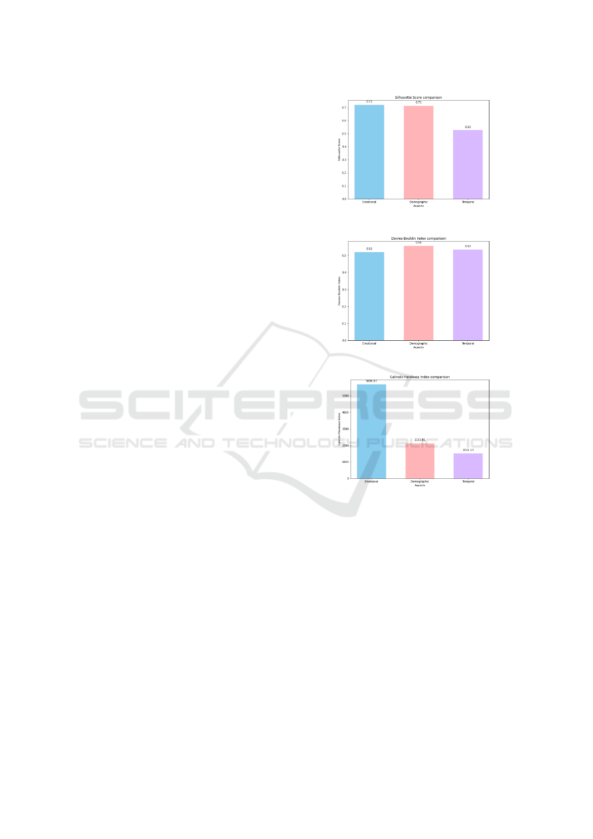
As detailed in Table 1 and visualized in Fig-

ures 2, 3 and 4, clustering of the demographic as-

pect, using MeanShift and 12 clusters, shows good

cohesion, with a silhouette score of 0.7119. The

low Davies-Bouldin index (0.5563) indicates well-

separated clusters, while the high Calinski-Harabasz

index (2132.8108) conﬁrms a marked separation be-

tween clusters. This suggests that the demographic

data fall into clear clusters.

With K-Means and 7 clusters, emotional aspect

achieves the best results compared to demographic

and temporal aspects. The silhouette score of 0.7199

and the lowest Davies-Bouldin index (0.5187) indi-

cate very compact, well-separated clusters. The high

Calinski-Harabasz score (5696.8659) reinforces this

distinction. Emotional data thus lend themselves well

to clustering, offering distinct groups.

Temporal clustering, performed with MeanShift

and 8 clusters, shows moderate results compared to

emotional and demographic aspects. The silhouette

score of 0.5256 and the Calinski-Harabasz index of

1521.1331 signal weaker cohesion and separation.

However, the Davies-Bouldin index of 0.5344 indi-

cates clusters that are still distinct, albeit less marked.

These results emphasize that temporal behaviors

are more complex to segment into homogeneous

groups and that the emotional data show the most dis-

tinct and cohesive clusters, with demographic data a

close second. The temporal aspect is more difﬁcult

to separate into well-deﬁned clusters, which reveals a

complexity in temporal patterns.

Figure 2: Silhouette Score.

Figure 3: Davies-Bouldin Index.

Figure 4: Calinski-Harabasz Index.

4.2 Contextual Based Collaborative

Filtering Stage Implementation

To highlight the robustness and performance of

our recommendation model, we implemented cross-

validation with various values of K-Folds and K-

Neighbors. This procedure enabled us to assess the

model’s stability and accuracy by dividing the data

into several subsets for alternate training and testing

phases.

We used RMSE (Root Mean Squared Error) and

MAE (Mean Absolute Error) as metrics to measure

the accuracy of the recommendations, RMSE being

more sensitive to large errors, while MAE provides a

measure of absolute deviations (Latrech et al., 2024).

As shown in Table 2 and Figure 5, the best per-

formance for K-Folds = 5 is achieved with 5 neigh-

Machine Learning Based Collaborative Filtering Using Jensen-Shannon Divergence for Context-Driven Recommendations

423

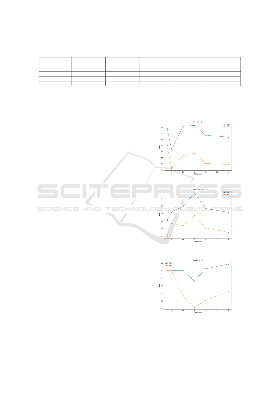
Table 1: Silhouette, Calinski-Harabasz and Davies-Bouldin metrics values for demographic, emotional and temporal contex-

tual aspects.

Aspect Algorithm

Optimal

Number of

Clusters

Silhouette Score

Davies-Bouldin

Index

Calinski-

Harabasz Index

Demographic MeanShift 12 0.7119 0.5563 2132.8108

Emotional K-Means 7 0.7199 0.5187 5696.8659

Temporal MeanShift 8 0.5256 0.5344 1521.1331

bors (RMSE: 0.9354, MAE: 0.6250), indicating good

accuracy. Beyond 5 neighbors, errors progressively

increase, with performance stabilizing at acceptable

rates, RMSE of 1.1438 and MAE of 0.6833, between

20 and 30 neighbors. Thus, a low number of neigh-

bors (5) offers the best accuracy for this conﬁguration.

With K-Folds set to 10, as indicated in Table 2

and visualized in Figure 6, optimal performance is

achieved with only 3 neighbors, where the RMSE

is particularly low (0.7071) and the MAE also low

(0.5000). However, as we move to 5 neighbors, the

RMSE increases slightly to 0.8165 and the MAE to

0.6667, which remains acceptable. A further increase

in the number of neighbors (to 10) results in a mod-

erate increase in RMSE (0.8975), while MAE de-

creases slightly. At 15 neighbors, the model shows

slightly larger errors, but as it increases to 20 and then

30 neighbors, performance improves slightly, even

reaching an RMSE of 0.8137 with 30 neighbors. For

K-Folds = 10, although the best results are obtained

with a low number of neighbors (3), conﬁgurations

with 20 and 30 neighbors also produce good perfor-

mance.

As described in Table 2 and depicted in Figure 7,

when the K-Folds = 15, the algorithm’s best perfor-

mance is obtained with 15 neighbors, for which the

RMSE reaches 0.8607 and the MAE is 0.5185. With

3 and 5 neighbors, RMSE and MAE remain constant

at high values (1.0000), which reﬂects less favorable

performance. With 10 neighbors, the MAE decreases

to 0.6667, but the RMSE remains high, while for 20

and 30 neighbors, the RMSE and MAE increase, even

to reach a performance degradation at 30 neighbors

with an RMSE of 1.0871. In this context of K-Folds

= 15, the optimum conﬁguration is around 15 neigh-

bors.

At K-Folds = 20, as highlighted in Table 2 and

illustrated by Figure 8, the algorithm performs opti-

mally with 10 neighbors, achieving a particularly low

RMSE of 0.5774 and a MAE of 0.3333, which makes

it the most accurate conﬁguration. At 3 and 5 neigh-

bors, the model maintains an RMSE of 0.7071 and

a MAE of 0.5000, but the 10-neighbor conﬁguration

performs better. Beyond 10 neighbors, RMSE and

MAE increase progressively, with values of 0.8034

for RMSE and 0.4636 for MAE at 15 neighbors. At

20 and 30 neighbors, the errors continue to increase,

with RMSE even reaching 1.0853 for 30 neighbors.

For K-Folds = 20, optimal performance is therefore

obtained with 10 neighbors, a conﬁguration that min-

imizes prediction errors.

Figure 5: RMSE and MAE by K-Neighbors for K-Folds=5.

Figure 6: RMSE and MAE by K-Neighbors for K-

Folds=10.

Figure 7: RMSE and MAE by K-Neighbors for K-

Folds=15.

Overall, the algorithm’s performance varies sig-

niﬁcantly as a function of K-Folds values and the

ICAART 2025 - 17th International Conference on Agents and Artiﬁcial Intelligence

424

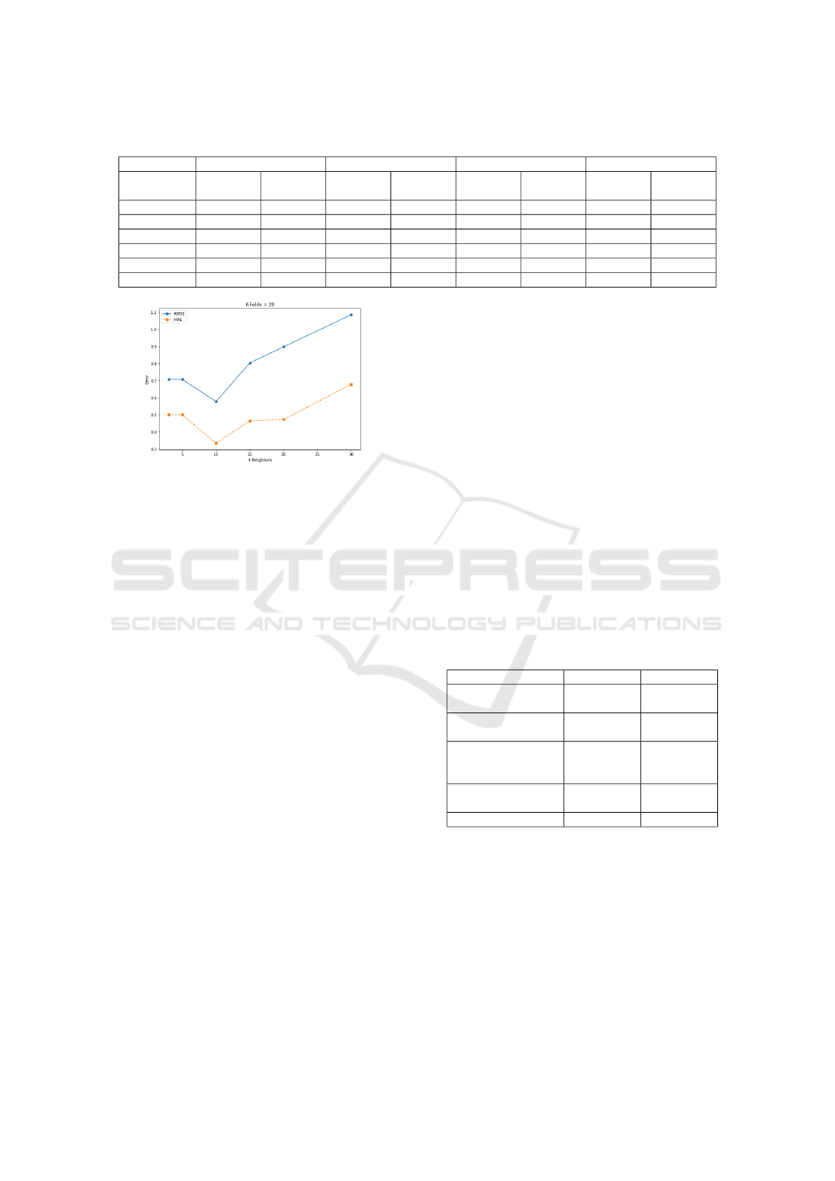
Table 2: RMSE and MAE comparison for different values of K-Folds and K-Neighbors.

K-Folds=5 K-Folds=10 K-Folds=15 K-Folds=20

K-

Neighbors

RMSE MAE RMSE MAE RMSE MAE RMSE MAE

3 1.2910 1.0000 0.7071 0.5000 1.0000 1.0000 0.7071 0.5000

5 0.9354 0.6250 0.8165 0.6667 1.0000 1.0000 0.7071 0.5000

10 1.3229 0.8333 0.8975 0.6389 1.0000 0.6667 0.5774 0.3333

15 1.3385 0.8750 1.0697 0.7693 0.8607 0.5185 0.8034 0.4636

20 1.1726 0.7083 0.8660 0.6071 1.0256 0.6074 0.8975 0.4722

30 1.1438 0.6833 0.8137 0.5509 1.0871 0.7273 1.0853 0.6778

Figure 8: RMSE and MAE by K-Neighbors for K-

Folds=20.

K-Neighbors selected for collaborative ﬁltering task.

For lower K-Folds values (5 and 10), the algorithm

achieves optimal performance with a reduced num-

ber of neighbors (3 to 5), which minimizes both

RMSE and MAE. This indicates that a small neigh-

borhood size is sufﬁcient for accurate predictions in

these conﬁgurations, because the model focuses more

efﬁciently on the closest relationships without overﬁt-

ting. On the other hand, for higher values of K-Folds

(15 and 20), the model performs better with an inter-

mediate number of neighbors, around 10 to 15 neigh-

bors, before the errors (RMSE and MAE) increase for

higher values of K-Neighbors. This behavior suggests

that with more detailed tests (i.e. more K-Folds), a

slightly larger set of neighbors can capture subtle vari-

ations in user preferences, while retaining good gen-

eralization.

• Baseline Methods

To highlight the performance of our model, we com-

pared it to other recommendation approaches imple-

mented on LDOS-CoMoDa dataset. Table 3 sum-

marizes the results achieved by the presented ap-

proaches.

■ KCAMF (Patil et al., 2022): In this research, the

authors proposed an innovative kernel-based loss

function to enhance matrix factorization optimiza-

tion in a non-linear projection rating space, with

optimal handling of context multiplicity.

■ CBMF (Casillo et al., 2022): In this paper, the

authors developed a contextual recommendation

system based on the concept of integrated context.

This system optimizes recommendation personal-

ization by directly incorporating relevant contex-

tual data into the recommendation generation pro-

cess.

■ Hybrid-IHSR (Unger and Tuzhilin, 2020): The

authors introduced an innovative hierarchical rep-

resentation method to capture latent contextual in-

formation, and understand users’ speciﬁc situa-

tions as they personalize recommendations. They

proposed a transformation process to structure un-

structured contextual information into hierarchi-

cal representations.

■ SVD++ (Kumar et al., 2014): This approach en-

riches the SVD++ factorization model with a so-

cial popularity factor based on implicit user feed-

back. This mechanism permits the capture of

users’ direct preferences and also the effect of an

item’s popularity within the community.

Table 3: RMSE and MAE comparison between models im-

plemented on LDOS-CoMoDa dataset.

Method RMSE MAE

KCAMF (Patil

et al., 2022)

0.9136 0.7177

CBMF (Casillo

et al., 2022)

1.0680 0.8386

Hybrid-IHSR

(Unger and

Tuzhilin, 2020)

1.2300 0.9700

SVD++ (Kumar

et al., 2014)

1.0571 0.8468

Our model 0.5774 0.3333

As shown in Table 3, our model achieved the low-

est RMSE and MAE values, conﬁrming its effective-

ness to integrate emotional, demographic, and tem-

poral contexts to deliver more context-driven recom-

mendations and accurately capture user preferences.

5 CONCLUSION

We introduced a machine learning-based context-

driven collaborative ﬁltering approach structured in

Machine Learning Based Collaborative Filtering Using Jensen-Shannon Divergence for Context-Driven Recommendations

425

three steps. First, a multi-aspect clustering analysis

is performed on the dataset, focusing on emotional,

demographic, and temporal aspects. Speciﬁc clus-

tering algorithms are applied to identify clusters and

generate probability distributions of users’ member-

ship, enabling a nuanced analysis of user proﬁles.

Second, the system constructs a normalized User-

User contextual weighted similarity matrix by cal-

culating similarity scores using the Jensen-Shannon

divergence method. These scores are dynamically

weighted to reﬂect the importance of each contex-

tual aspect, aggregated to compute global similar-

ity scores, and used to build the normalized matrix.

The ﬁnal step applies collaborative ﬁltering based on

the normalized matrix, identifying the N contextually

closest users to predict ratings for unrated items and

generate recommendations. Experiments conducted

on the LDOS-CoMoDa dataset demonstrated good

performance, with RMSE and MAE rates of 0.5774

and 0.3333, respectively. These results highlight the

model’s ability to deliver contextually personalized

suggestions tailored to variations in user preferences.

To enhance this approach, we aim to explore alter-

native divergence metrics beyond the Jensen-Shannon

divergence and apply the method to various datasets.

This comparative analysis will provide insights into

optimizing contextual recommendations and adapting

them to the speciﬁc characteristics of user proﬁles.

REFERENCES

Adomavicius, G. and Tuzhilin, A. (2010). Context-aware

recommender systems. In Recommender systems

handbook, pages 217–253. Springer.

Cali

nski, T. and Harabasz, J. (1974). A dendrite method for

cluster analysis. Communications in Statistics-theory

and Methods, 3(1):1–27.

Casillo, M., Gupta, B. B., Lombardi, M., Lorusso, A., San-

taniello, D., and Valentino, C. (2022). Context aware

recommender systems: A novel approach based on

matrix factorization and contextual bias. Electronics,

11(7):1003.

Fukunaga, K. and Hostetler, L. (1975). The estimation of

the gradient of a density function, with applications in

pattern recognition. IEEE Transactions on informa-

tion theory, 21(1):32–40.

Karabila, I., Darraz, N., El-Ansari, A., Alami, N., and

El Mallahi, M. (2023). Enhancing collaborative

ﬁltering-based recommender system using sentiment

analysis. Future Internet, 15(7):235.

Karatzoglou, A., Amatriain, X., Baltrunas, L., and

Oliver, N. (2010). Multiverse recommendation: n-

dimensional tensor factorization for context-aware

collaborative ﬁltering. In Proceedings of the fourth

ACM conference on Recommender systems, pages 79–

86.

sir, A., Odic, A., Kunaver, M., Tkalcic, M., and Tasic,

J. F. (2011). Database for contextual personalization.

Elektrotehni

ski vestnik, 78(5):270–274.

Kullback, S. and Leibler, R. A. (1951). On information

and sufﬁciency. The annals of mathematical statistics,

22(1):79–86.

Kumar, R., Verma, B., and Rastogi, S. S. (2014). Social

popularity based svd++ recommender system. Inter-

national Journal of Computer Applications, 87(14).

Latrech, J., Kodia, Z., and Ben Azzouna, N. (2024). Codﬁ-

dl: a hybrid recommender system combining en-

hanced collaborative and demographic ﬁltering based

on deep learning. The Journal of Supercomputing,

80(1):1160–1182.

Lin, J. (1991). Divergence measures based on the shannon

entropy. IEEE Transactions on Information theory,

37(1):145–151.

Lloyd, S. (1982). Least squares quantization in pcm. IEEE

transactions on information theory, 28(2):129–137.

Pagano, R., Cremonesi, P., Larson, M., Hidasi, B., Tikk,

D., Karatzoglou, A., and Quadrana, M. (2016). The

contextual turn: From context-aware to context-driven

recommender systems. In Proceedings of the 10th

ACM conference on recommender systems, pages

249–252.

Palacio-Ni

no, J.-O. and Berzal, F. (2019). Evaluation

metrics for unsupervised learning algorithms. arXiv

preprint arXiv:1905.05667.

Patil, V. A., Chapaneri, S. V., and Jayaswal, D. J. (2022).

Kernel-based matrix factorization with weighted reg-

ularization for context-aware recommender systems.

IEEE Access, 10:75581–75595.

Said, A., De Luca, E. W., and Albayrak, S. (2011). Infer-

ring contextual user proﬁles-improving recommender

performance. In Proceedings of the 3rd RecSys work-

shop on context-aware recommender systems, volume

791.

Unger, M. and Tuzhilin, A. (2020). Hierarchical latent

context representation for context-aware recommen-

dations. IEEE Transactions on Knowledge and Data

Engineering, 34(7):3322–3334.

Wijaya, Y. A., Kurniady, D. A., Setyanto, E., Tarihoran,

W. S., Rusmana, D., and Rahim, R. (2021). Davies

bouldin index algorithm for optimizing clustering case

studies mapping school facilities. TEM J, 10(3):1099–

1103.

ICAART 2025 - 17th International Conference on Agents and Artiﬁcial Intelligence

426