A Comparative Analysis of Hyperparameter Effects on CNN

Architectures for Facial Emotion Recognition

Benjamin Grillo

, Maria Kontorinaki

and Fiona Sammut

Department of Statistics & Operations Research, University of Malta, Msida, Malta

Keywords: Facial Emotion Recognition, Convolutional Neural Networks, Custom Network Architecture, Image Data,

Classification, Hyperparameter Effects, Model Performance.

Abstract: This study investigates facial emotion recognition, an area of computer vision that involves identifying human

emotions from facial expressions. It approaches facial emotion recognition as a classification task using

labelled images. More specifically, we use the FER2013 dataset and employ Convolutional Neural Networks

due to their capacity to efficiently process and extract hierarchical features from image data. This research

utilises custom network architectures to compare the impact of various hyperparameters - such as the number

of convolutional layers, regularisation parameters, and learning rates - on model performance.

Hyperparameters are systematically tuned to determine their effects on accuracy and overall performance.

According to various studies, the best-performing models on the FER2013 dataset surpass human-level

performance, which is between 65% and 68%. While our models did not achieve the best-reported accuracy

in literature, the findings still provide valuable insights into hyperparameter optimisation for facial emotion

recognition, demonstrating the impact of different configurations on model performance and contributing to

ongoing research in this area.

1 INTRODUCTION

Facial Emotion Recognition (FER) is a field of study

in computer vision that focuses on identifying human

emotions from facial expressions, which are essential

for non-verbal communication. It relies on advanced

techniques such as deep learning and facial feature

extraction to detect and analyse subtle changes in

facial muscles. FER has gained significant attention

across various fields, including human-computer

interaction, clinical diagnostics, and behavioural

analysis, according to (Khan et al., 2013; Sariyanidi

et al., 2015). In clinical settings, it is used for

monitoring mental health conditions, such as

detecting early signs of depression or anxiety. In

marketing, FER helps assess customer reactions to

products and advertisements, providing real-time

insights into consumer behaviour. Its applications are

rapidly expanding, particularly in interactive systems

such as virtual assistants and social robots, where

accurate emotion detection enhances user interaction

https://orcid.org/0009-0003-6213-6632

https://orcid.org/0000-0002-1373-5140

https://orcid.org/0000-0002-4605-9185

by making systems more intuitive and responsive.

Additionally, FER is being integrated into security

systems for lie detection and threat assessment,

offering new dimensions of situational awareness.

While FER technology presents many benefits, it also

raises ethical concerns regarding privacy and the

potential misuse of biometric data.

This study uses the FER2013 dataset, a widely

recognised benchmark introduced at ICML 2013.

FER2013 consists of facial images classified into

seven emotion classes - anger, disgust, fear, happy,

neutral, sad and surprise. Although other datasets

such as CK+, JAFFE, or KDEF are available for

studies related to FER, in this study, we focused

solely on FER2013 for several legitimate reasons.

First, FER2013 contains over 35,000 images, making

it significantly more prominent than other datasets,

such as CK+ and JAFFE, with only a few hundred

samples. This larger dataset provides more data for

training deep learning models, which typically

perform better with extensive, diverse datasets.

Grillo, B., Kontorinaki, M. and Sammut, F.

A Comparative Analysis of Hyperparameter Effects on CNN Architectures for Facial Emotion Recognition.

DOI: 10.5220/0013146900003905

Paper published under CC license (CC BY-NC-ND 4.0)

In Proceedings of the 14th International Conference on Pattern Recognition Applications and Methods (ICPRAM 2025), pages 587-596

ISBN: 978-989-758-730-6; ISSN: 2184-4313

587

Second, FER2013 is collected in real-world

conditions, featuring images captured in uncontrolled

environments with varying lighting, angles, and

backgrounds. This makes it more representative of

real-world scenarios compared to more controlled,

posed datasets like CK+ and JAFFE, which may not

generalise as well to everyday applications.

Additionally, FER2013 is a widely used benchmark

in the field, allowing researchers to compare their

results with existing studies, ensuring consistency

and reproducibility. The larger size and diversity also

reduce the risk of overfitting, making models more

robust in practical applications. Furthermore, using a

single dataset simplifies preprocessing and reduces

computational demands, which is particularly

important when training complex models. In this

study, we also performed a preliminary cleaning of

the FER2013 dataset to improve its quality, though a

more detailed explanation of this process is provided

in Section 2.1. Finally, FER2013 includes a balanced

distribution of common emotions, providing a more

comprehensive test bed for emotion recognition

models, whereas other datasets may suffer from class

imbalance or limited categories. (Tang, 2015) states

that humans correctly identify the emotions in the

FER2013 images between 65% and 68% of the time,

demonstrating the inherent difficulty of emotion

recognition when working with this dataset.

Recent advances in deep learning, particularly

with Convolutional Neural Networks (CNNs), have

led to significant improvements in FER. CNNs are

especially well-suited for image-based tasks due to

their ability to automatically learn spatial hierarchies

of features, removing the need for manual feature

extraction. The literature on FER demonstrates the

effectiveness of CNNs in handling the complexities

stemming from the use of the FER2013 dataset.

(Khaireddin & Chen, 2021) achieved a 73.28%

accuracy on the FER2013 dataset using a fine-tuned

VGGNet architecture, illustrating the potential of

deep CNN models in emotion recognition tasks.

(Liliana, 2019) explored the detection of facial action

units using CNNs and reached a 92.81% accuracy on

the CK+ dataset, emphasising CNNs' ability to

capture subtle facial movements indicative of

emotions. (Hassouneh et al., 2020) extended FER by

integrating electroencephalograph signals with CNNs

and Long Short-Term Memory (LSTM) networks,

highlighting the potential of combining CNNs with

other modalities for enhanced emotion recognition.

Similarly, (Akhand et al., 2021) applied transfer

learning to pre-trained CNNs, fine-tuning models for

emotion-specific tasks, and reported accuracies of

96.51% on the KDEF dataset and 99.52% on the

JAFFE dataset. These studies demonstrate the

adaptability and effectiveness of CNNs in FER across

various datasets and configurations.

In this work, custom CNN architectures are

developed and optimised to improve the accuracy of

FER using the FER2013 dataset. Different

hyperparameters and techniques are experimented on

to observe their effects on the model’s performance

and assess how various configurations influence the

results. Additionally, various architectural

components are explored. While the architectures we

employed did not achieve the highest reported

accuracy compared to the best models in the

literature, we believe our work offers significant

contributions. Specifically, we conducted extensive

experiments testing a wide range of hyperparameter

configurations, providing valuable insights into how

these variations impact model accuracy. This detailed

exploration of hyperparameter tuning - covering

aspects such as architectural depth, augmentation

techniques, learning rate, batch size, dropout rate, and

other regularisation methods - offers a unique

perspective that is often overlooked in studies focused

solely on peak performance. By systematically

analysing how different hyperparameter values

influence model behaviour, our study provides a

deeper understanding of the intricacies involved in

optimising CNNs for FER tasks. Such insights are

critical for researchers looking to refine existing

models or develop new architectures. Additionally,

the findings from our hyperparameter analysis serve

as a practical guide for future research, offering

actionable recommendations for tuning CNNs in this

domain. We believe that this contribution fills an

important gap in the literature and deserves attention

for advancing both practical applications and

theoretical understanding of FER model optimisation.

2 EXPERIMENTAL RESULTS

This section details the dataset used, as well as the

experimental setup, including data pre-processing,

model architecture, and hyperparameter tuning.

Various experiments were conducted to compare the

effects of different approaches, such as data

augmentation techniques, batch sizes, learning rate

scheduling, and regularisation methods. Additionally,

comparisons between basic and deeper architectures

were made, and Keras Tuner (O’Malley, T., et al,

2019) was employed for fine-tuning

hyperparameters. These steps were taken to optimise

model performance and evaluate how each

modification impacted the results.

ICPRAM 2025 - 14th International Conference on Pattern Recognition Applications and Methods

588

2.1 Standardised Procedures

This section outlines the standardised procedures

applied across all experiments. These practices

remained consistent throughout the study to ensure

comparability and maintain methodological rigor.

The Facial Expression Recognition 2013

(FER2013) dataset contains 35,887 grayscale images

at a resolution of 48 × 48 pixels, divided into training

and testing sets, where each image is labelled with

one of seven emotions: anger, disgust, fear,

happiness, neutral, sadness, and surprise. Although

the dataset is widely utilised in facial expression

recognition research, it presents some limitations,

including mislabelled or irrelevant images. To this

end, a manual data cleaning process was conducted

on both sets. This involved systematically reviewing

each image and removing those without a visible face.

By manually verifying the dataset, we ensured that

irrelevant or extremely noisy images were eliminated.

This process enhances the training reliability, leading

to more accurate model evaluation. The cleaned

version of the dataset has been uploaded to Kaggle for

public use (Grillo, 2024).

For each experiment, input images were re-scaled

during pre-processing using the Keras (Chollet &

others, 2015) class ImageDataGenerator. This

normalises pixel values to a range of 0 to 1, instead of

0 to 255. This is a common practice as it reduces

skewness and variance, leading to improved model

performance and faster convergence during training.

The categorical cross-entropy loss function was

used throughout the experiments, as it is well-suited

for multi-class classification tasks such as FER. This

function computes the negative log-likelihood of the

correct class, penalising the model when predicted

probabilities deviate from true labels. Applying a

logarithmic penalty to misclassifications helps the

model assign the highest probability to the correct

class while managing the distribution across other

classes. This enhances the model’s ability to capture

subtle distinctions between facial expressions,

leading to precise weight updates during training and

improving classification accuracy on unseen images.

The Adam (Adaptive Moment Estimation)

optimiser, introduced by (Kingma & Ba, 2017), was

used for all experiments in this study due to its

efficiency and adaptability in handling noisy

gradients and varying learning rates. Adam improves

upon traditional Stochastic Gradient Descent by

adjusting learning rates for each parameter

individually, based on the first and second moments

of the gradients. This allows for dynamic learning rate

adaptation, which enhances convergence speed and

stability. Adam's ability to maintain adaptive learning

rates throughout training makes it particularly

effective for tasks like FER, where variations in data

can lead to challenges in gradient consistency.

Finally, when choosing the most appropriate

hyperparameter values for our FER application, we

focus on two key performance metrics: test accuracy

and precision. Accuracy measures the overall

proportion of images correctly classified by the

model. Precision reflects the quality of the model's

positive predictions. Specifically, we use a weighted

average of precision across all classes, where each

class's precision is weighted by its frequency in the

dataset. For each class, precision is the proportion of

true positive predictions (correct classifications)

among all the positive predictions made by the model

for that class. This ensures that the model is not only

accurate overall but also reliable in making correct

positive predictions for each category.

2.2 Experimental Setup

This section presents the configurations tested to

evaluate their effect on model performance. A variety

of model architectures, hyperparameters, and training

strategies were systematically explored to understand

how adjustments in data augmentation, batch sizes,

learning rate schedules, regularisation techniques,

and architecture depth impacted FER effectiveness.

2.2.1 Model Architectures

For this study, two CNN architectures were

developed: a basic model serves for initial testing and

comparative analysis, and a deeper model for

improved performance through advanced feature

extraction. Both follow a sequential structure for

straightforward layer stacking and flexibility. Minor

configuration adjustments were applied in certain

experiments, as detailed in later sections.

The basic architecture processes 48×48 grayscale

images through four convolutional blocks. Each

block includes a 3×3 convolutional layer, with a stride

of 1 and no padding, prioritising central features over

edge details. Batch normalisation, ReLU activation,

and 2×2 max pooling are applied in each block, with

the number of filters increasing from 32 to 256. A

Global Average Pooling (GAP) layer precedes a

dense layer with 256 units and dropout, followed by

a softmax layer for classification into seven

categories. With 0.47 million parameters, this

architecture provides a computationally efficient

baseline for testing and iterative development.

A Comparative Analysis of Hyperparameter Effects on CNN Architectures for Facial Emotion Recognition

589

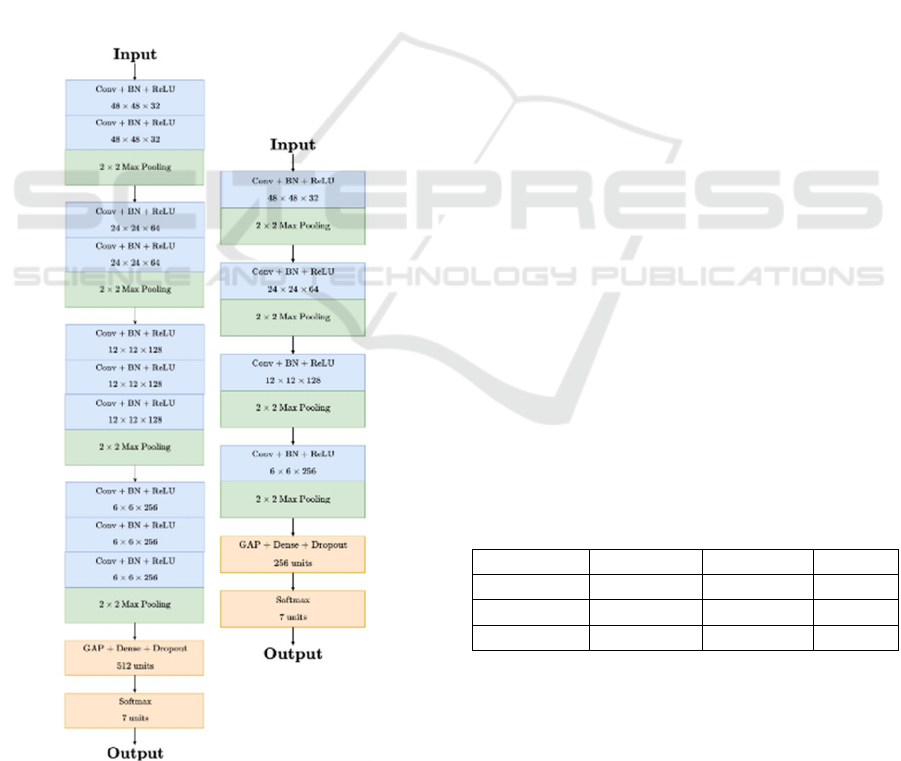
The deeper architecture begins with an input layer

for 48×48 grayscale images and consists of four

convolutional blocks. The first two blocks have two

3×3 convolutional layers, while the third and fourth

blocks include three layers. As in the basic model,

batch normalisation, ReLU activation, and 2×2 max

pooling are applied. Filter sizes double progressively

from 32 to 256. A GAP layer connects to a dense layer

with 512 units and dropout, culminating in a softmax

layer for classification. With 2.05 million parameters,

this adapts elements of VGG16 (Simonyan &

Zisserman, 2015), optimising for low-resolution FER

data while maintaining efficiency.

Both architectures have significantly fewer

parameters than popular models such as VGG16 (138

million) and Inception (6.99 million) (Szegedy et al.,

2014). The deeper model is also more lightweight

than MobileNetV2, which has 3.5 million parameters

(Sandler et al., 2019). Figure 1 illustrates the

structures of these architectures.

Figure 1: Basic (right) and Deeper (left) Architectures.

2.2.2 On-the-Fly vs. Static Augmentation

Experiments using the basic architecture were

conducted on the FER2013 dataset to evaluate the

effects of data augmentation strategies. The model

was trained with a batch size of 64 for up to 100

epochs, with early stopping with a patience of 10 to

prevent overfitting. 20% of the training set was

reserved for validation, with validation loss as the

early stopping metric.

For on-the-fly augmentation, transformations

such as horizontal flipping (50% chance), rotations

(±10°), width and height shifts (up to 20%), and

zooming (80%-120%) in real-time during training

were applied. These were derived from (Khaireddin

& Chen, 2021). These augmentations introduced

variability while keeping the dataset size unchanged.

Static augmentation applied a horizontal flip

(50% chance) and a ±30° rotation to each image,

inflating the dataset by about 250%. Augmented

images were saved to the training directory, making

this setup more memory-intensive and limiting the

variety of transformations possible. A third

experiment with no augmentation was also set up.

On-the-fly augmentation was the most effective,

achieving the highest test accuracy and precision,

while having the smallest loss. This method

introduced variability during training without

increasing memory requirements, enabling a wider

range of transformations and better performance.

Static augmentation, despite using pre-augmented

images, resulted in lower metrics and more

misclassifications. All methods struggled with the

disgust class, with only the on-the-fly model correctly

classifying one instance. From a computational

standpoint, static augmentation was the most

resource-intensive. On-the-fly, while taking longer

than no augmentation, offered better accuracy and

generalisation and will be used in all subsequent

experiments. Table 1 summarises the results.

Table 1: Results of data augmentation experiments.

Type Test Loss Test Acc. Prec.

No Aug 1.602 0.5292 0.5872

On-the-fly 1.161 0.5586 0.5976

Static 1.614 0.5248 0.1748

2.2.3 Optimising Batch Size

These experiments were aimed at isolating the effects

of batch size variation on model performance and

identifying the optimal batch size. Batch sizes of 8,

16, 32, 64, and 128 were tested. A grid search was

conducted, maintaining basic model architecture and

ICPRAM 2025 - 14th International Conference on Pattern Recognition Applications and Methods

590

on-the-fly augmentation, with a maximum of 100

epochs and early stopping with a patience of 12.

Batch sizes 16 and 8 were closely matched in

overall performance; however, batch size 16 was

chosen for subsequent experiments as it had superior

classification of underrepresented classes. Loss and

accuracy plots indicated that as batch sizes increased,

oscillations became more pronounced, suggesting

greater variance and reduced stability in training, as

illustrated in Figure 2. Larger batch sizes, like 64 and

128, struggled with underrepresented classes, with

batch size 128 struggling particularly with the fear

category and classifying one image in the disgust

class. Based on these findings, batch size 16 will be

used in all subsequent experiments due to its balance

between stability and accuracy across all classes.

Refer to Table 2 for a summary of results.

Figure 2: Loss and accuracy plots of experiments with batch

sizes 8 (top) and 16 (bottom).

Table 2: Results of batch size grid search.

Batch Size Test Loss Test Acc. Prec.

8 1.066 0.6233 0.6344

16 1.008 0.6211 0.6345

32 1.087 0.6071 0.6208

64 1.161 0.5586 0.5976

128 1.591 0.4937 0.6094

2.2.4 Experimenting with Learning Rate,

Validation Set Size Reduction and

Further Regularisation

This section evaluates the impact of learning rate

scheduling techniques, including staircase

exponential decay and dynamic adjustments using

ReduceLROnPlateau

, on the basic and deeper

model. The effects on training and validation metrics

are also analysed, along with the responsiveness of

these strategies on a reduced validation set. Here we

also experiment with L2 regularisation to see how the

model reacts.

2.2.5 Using Exponential Staircase Decay

with Basic Architecture

The first set of experiments in this section examined

the effect of exponential staircase decay on

performance using the basic architecture. The initial

learning rate was set at 0.001, with decay occurring

every

steps_per_epoch*10

at a rate of 0.95, where

steps_per_epoch

represents the number of batches

processed per epoch. This configuration yielded a test

accuracy of 60.98%, which did not surpass the best

accuracy of the previous experiments. The respective

confusion matrix indicated more misclassifications,

suggesting the adjustments did not enhance the

model's discriminative capacity. Additionally, loss

and accuracy plots showed similar oscillation patterns

to previous trials using the same batch size, indicating

that the learning rate modifications failed to smooth

the convergence process or improve training stability.

Two additional experiments tested different decay

schedules. The first adopted a less aggressive rate of

0.96, applied every

steps_per_epoch*8,

resulting

in an accuracy of 60.03%. This facilitated gradual

convergence but did not significantly improve

performance. The second implemented a more

aggressive decay rate of 0.94, applied every

steps_per_epoch*12

, leading to an improved

accuracy of 63.81%. This slower, more aggressive

decay schedule improved performance, particularly

in underrepresented emotions and demonstrated more

stable convergence patterns. The improved

performance on the disgust class highlighted the

effectiveness of a slower decay in learning subtle

features. The results are summarised in Table 3.

Experiments with other parameters produced inferior

results and were not explored further.

Overall, the experiments emphasise the

importance of optimising learning rate decay

strategies to improve model stability, generalisation,

and accuracy, especially for underrepresented classes

Table 3: Summary of results of experiments using

exponential staircase decay with the basic architecture.

Decay

Fre

Decay

Rate

Test

Loss

Test

Acc.

Prec.

8 0.96 1.095 0.6003 0.6265

10 0.95 1.048 0.6098 0.6196

12 0.94 1.010 0.6381 0.6417

A Comparative Analysis of Hyperparameter Effects on CNN Architectures for Facial Emotion Recognition

591

Figure 3: Loss and accuracy plots of the experiments using

the basic (top) and deeper (bottom) architectures, with

exponential staircase decay (0.94 /steps_per_epoch*12).

Figure 4: Confusion matrices of basic (left) and deeper

(right) architectures, with exponential staircase decay

applied at a rate of 0.94 every steps_per_epoch*12.

2.2.6 Using Exponential Staircase Decay

with Deeper Architecture

This section extends previous findings by applying

the best parameters to the deeper model architecture.

The model was trained for up to 150 epochs, with

early stopping after 15 epochs. While more

computationally demanding, the deeper model

improved performance, achieving 66.33% accuracy.

The deeper model also outperformed the basic

model in overall precision and also across most classes

individually, particularly improving in classifying the

underrepresented disgust class, as shown in the

confusion matrix in Figure 4. Loss and accuracy plots

showed greater stability in training, with reduced

oscillations compared to the basic model, suggesting

improved training dynamics and reduced instability.

Overfitting was also present in both models, as seen in

the plots of Figure 3. These results suggest the deeper

model’s enhanced capacity to recognise subtle features

and provide consistent performance, positioning it as a

strong candidate for further development.

2.2.7 Reducing Validation Set Size

This section investigates reducing the validation set

size from 20% to 10%, primarily to provide more

training data while still maintaining sufficient metrics

for early stopping. Both the basic and deeper models

were tested using a staircase exponential decay with

training extended to 300 epochs and early stopping

patience set to 30 to accommodate for increased

variability from the smaller validation set.

The basic model required 144 epochs with the

smaller validation set, compared to 83 with the larger

set, indicating increased computational demands. The

deeper model showed minimal change in training

duration. Accuracy improved to 65.59% for the basic

model and 66.44% for the deeper model. While both

models saw small gains in precision, the deeper

model did not consistently outperform the basic

model. Surprisingly, the basic model with a reduced

validation set performed better in classifying

underrepresented emotions like disgust, correctly

identifying 65 of 111 instances, as indicated by the

matrix in Figure 5. Loss and accuracy plots also

indicated greater training stability in the deeper

model. Reducing the size of the validation set

benefitted the basic model more significantly than the

deeper model.

2.2.8 Implementing L2 Regularisation

In an effort to further improve generalisation, L2

regularisation with a coefficient of 1e-3 was applied

to each convolutional layer and to the dense layer of

the deeper model. This value was chosen based on the

suggestions of (Goodfellow et al., 2016). This

technique adds a penalty for larger weights to the loss

function, encouraging the model to learn more

general patterns. However, the model showed

considerable variation in emotion classification and

performed the worst overall. While it successfully

identified classes like happy and surprise, it failed to

recognise disgust and also underperformed in fear and

angry. The model also displayed a strong bias toward

the neutral class, as indicated by the confusion matrix

in Figure 7. The model frequently misclassified other

Figure 5: Confusion matrices of basic (left) and deeper

(right) models, with exponential staircase decay (0.94 /

every steps_per_epoch*12) and a smaller validation set.

ICPRAM 2025 - 14th International Conference on Pattern Recognition Applications and Methods

592

emotions as neutral, where the features are often less

distinct and closer to the average across all classes.

The loss and accuracy plots in Figure 6 revealed

erratic training behaviour, with a sharp spike in

training loss and high variability in validation

accuracy, indicating poor learning and generalisation.

Figure 6: Loss and accuracy plots of the experiment with

L2 regularisation.

Figure 7: Confusion matrix of experiment with L2

regularisation.

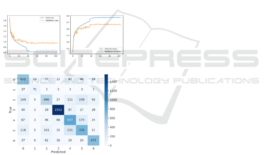
2.2.9 Implementing ReduceLRonPlateau

Here, we examine the use of the

ReduceLROnPlateau

callback for dynamic learning

rate adjustment, which reduces the learning rate when

no improvement in validation loss is observed over a

set number of epochs. Three experiments were

conducted on the deeper model, all with a patience of

10 epochs and varying the reduction factor: 0.1, 0.12,

and 0.08. All experiments used 10% of the training

set for validation and trained for up to 300 epochs

with early stopping patience at 30 epochs.

Performance across the experiments was closely

matched, with the third experiment, using a reduction

factor of 0.08, achieving the highest accuracy at

68.45%, compared to 68.21% and 66.77% in the other

two, as seen in Table 4. This suggests a moderate

reduction factor improves performance without

sacrificing stability. Evaluation metrics for the

classification report show

ReduceLROnPlateau

outperformed exponential decay, achieving better

metrics, particularly in underrepresented classes.

Figures 8 and 9 show the loss and accuracy plots

and confusion matrix, of the best performing model.

Table 4: Summary of results of ReduceLROnPlateau

experiments.

Reduction

Rate

Patience Test

Loss

Test

Acc.

Prec.

0.08 10 0.969 0.6845 0.6853

0.1 10 0.958 0.6821 0.6853

0.12 10 0.971 0.6677 0.6689

Figure 8: Loss and accuracy plots of the best-performing

model from this series of experiments.

Figure 9: Confusion matrix of the best-performing model

from this series of experiments.

2.2.10 Hyperparameter Tuning Using Keras

Tuner

Keras Tuner (O’Malley, T., et al, 2019) is an

advanced framework for hyperparameter tuning in

TensorFlow and Keras models. It employs algorithms

such as Random Search, Hyperband (L. Li et al.,

2018) and Bayesian Optimisation to explore various

hyperparameter configurations. A hypermodel,

serving as a flexible model framework, is defined

with a search space for the hyperparameters. Keras

Tuner then iteratively builds and evaluates models

based on these configurations, using techniques like

early stopping to improve efficiency. In this section,

four targeted experiments are conducted, each

focusing on optimising a specific aspect of the model.

The first experiment aimed to find the optimal

number of dense layer units and initial learning rate

using the

Hyperband

class to balance model capacity

A Comparative Analysis of Hyperparameter Effects on CNN Architectures for Facial Emotion Recognition

593

and convergence speed. Dense layer sizes of 256,

512, 1024, 2048, and 4096 were explored, alongside

learning rates of 0.01, 0.001, and 0.0001. The tuning

ran for up to 50 epochs, with early stopping after 5

epochs without validation loss improvement, and

dynamic learning rate adjustments using

ReduceLROnPlateau. The optimal configuration

was 1024 dense units and a learning rate of 0.0001.

The process took five hours and 48 minutes.

The second experiment focused on optimising

dropout rates using

Hyperband class, to reduce

overfitting while retaining expressiveness. Dropout

rates from 0% to 50% in convolutional layers and

20% to 70% in the dense layer were tested. Early

stopping based on validation loss was applied, with

configurations evaluated for up to 50 epochs. After

nearly 28 hours, the optimal configuration was found

- no dropout for the 32-filter and 128-filter layers,

25% for the 64-filter layer, 5% for the 256-filter layer,

and 25% for the dense layer.

The third optimised batch normalisation

momentum and found a better balance between

stability and adaptability during training.

Hyperband

was used, testing values between 0.89 and 0.99. The

tuner dynamically adjusted the number of epochs up

to 50, with early stopping after 10 epochs of no

validation loss improvement. The optimal value was

0.91, and the search completed in 1 hour and 39

minutes, due to the smaller search space.

The final experiment aimed to optimise the L2

regularisation coefficient to better control overfitting.

RandomSearch class was used to test values from 1e-

6 to 1e-3 . The experiment ran over four trials of 30

epochs, with dynamic learning rate adjustments via

the

ReduceLROnPlateau callback. The optimal L2

regularisation coefficient values were much smaller

than those used in the experiment of Section 2.3.3.4.

The optimal coefficients were found to be 1e-3 for

the first 32-filter layer, 1e-6 for the second, 1e-4 for

the 64-filter and 128-filter layers, 1e-4 and 1e-6 for

the 256-filter layers, and 1e-5 for the dense layer. The

process ran for 7 hours.

Following these searches, we combined optimal

hyperparameters to maximise performance in the

deeper model. Dropout was applied after batch

normalisation, as recommended by (X. Li et al., 2018),

to prevent variance inconsistency. All experiments

were capped at 300 epochs with early stopping after 30

epochs of no validation loss improvement, and

dynamic learning rate adjustments applied.

In the first experiment, we increased the dense

units from 512 to 1024 to evaluate the impact of

capacity on performance. This had no significant

impact, with an accuracy of 66.52%, similar to prior

results. The model trained for 81 epochs without

added computational cost. In the second experiment,

L2 regularisation and batch normalisation momentum

improved accuracy to 67.36% with training extending

to 141 epochs. Additional regularisation reduced

overfitting compared to the first experiment.

In the third and fourth experiments, learning rate

was reduced to 0.0001, following a warm-up at 0.001

for 8 epochs, as suggested by the tuner. The third,

with 1024 dense units, completed in 119 epochs,

while the fourth, adding batch normalisation

momentum and L2 regularisation, took 126. The

fourth showed the best generalisation, with less

overfitting than the others.

2.2.11 Further Architectural Changes

In this section, we experimented further with

architectural changes to the deeper model, including

the addition of fully-connected layers, convolutional

layers, and adjustments to the block structure. This

was to assess whether increasing the network's

capacity, through additional parameters and depth,

would lead to an improved performance.

Table 5 summarises the configurations of the

experiments. The rows represent convolutional

blocks with respective filter sizes and dense layers.

The values correspond to the number of filters in the

block or the number of units in the dense layer. The

final row is the total number of parameters, in

millions,. Results are summarised in Table 6.

Table 5: Architectural configurations of the experiments.

Layer

Type

Exp

Conv 32 2 2 2 0 2

Conv 64 2 2 2 2 2

Conv 128 3 3 3 2 3

Conv 256 3 3 3 3 3

Conv 256 0 0 0 0 3

Conv 512 0 0 0 3 0

Dense 1 1024 2048 256 2048 2048

Dense 2 1024 1024 2048 1024 1024

Params 3.23 4.55 2.52 10.80 6.31

Table 6: Summary of results of experiments in this section.

Exp no. Test Loss Test Acc. Prec.

1 0.921 0.6683 0.6677

2 0.933 0.6772 0.6767

3 0.904 0.6700 0.6707

4 0.938 0.6933 0.6929

5 0.952 0.6735 0.6748

ICPRAM 2025 - 14th International Conference on Pattern Recognition Applications and Methods

594

From the loss and accuracy plots, all experiments

exhibited similar learning behaviours. Experiment 4,

the most complex, achieved the best results, with the

highest test accuracy, precision, and disgust class

performance. This suggests that additional layers and

parameters improved the model’s ability.

Experiment 3, with the fewest parameters, had the

lowest test loss, indicating good generalisation

despite having a slightly lower accuracy than

Experiment 4. This shows that simpler models can

still be competitive for generalisation, though they

may struggle with complex or underrepresented data.

Experiment 5, despite having more parameters

than Experiment 3, achieved almost the same

accuracy. This suggests increasing parameters does

not guarantee better performance and highlights

diminishing returns from added complexity without

effective optimisation. Figures 10 and 11 show the

loss and accuracy plots and confusion matrix of

Experiment 4, the best-performing model.

Figure 10: Loss and Accuracy Plot of Experiment 4.

Figure 11: Confusion Matrix of Experiment 4.

3 CONCLUSION

This study investigated CNNs for FER using a clean

version of the FER2013 dataset, focusing on the

impact of architectural modifications, learning rate

schedules, and regularisation techniques. Key

findings demonstrated the benefits of on-the-fly

augmentation, optimal batch sizes, and dynamic

learning rate adjustment. Hyperparameter tuning

using Keras Tuner optimised dense units, learning

rates, dropout, and L2 regularisation, providing

insights into balancing performance and efficiency.

While our models did not achieve the highest

reported accuracy, the findings contribute to

understanding how hyperparameter configurations

affect performance and generalisation. Theoretical

insights suggest that certain architectural

modifications, such as deeper convolutional layers

and dropout placement, improve feature extraction

and stability, which may generalise to other FER

problems or low-resolution datasets. However, the

performance gap compared to state-of-the-art models

may be attributed to the limited complexity of the

architectures used, suggesting further exploration of

deeper or more advanced designs.

Future work should explore the generalisability of

these findings to other architectures, datasets, and

tasks. Assessing performance variability across

repeated runs, different splits of training data, and

random initialisations would strengthen the

robustness of comparative results. Additionally,

addressing class imbalance through weighted classes

and extending augmentation techniques could further

improve generalisation. Validation strategies like k-

fold cross-validation and more extensive architectural

refinements—such as filter size variations or

alternative optimisers—may provide deeper insights

into model behaviour.

REFERENCES

Akhand, M. A. H., Roy, S., Siddique, N., Kamal, M. A. S.,

& Shimamura, T. (2021). Facial Emotion Recognition

Using Transfer Learning in the Deep CNN. Electronics,

10, 1036.

Chollet, F. & others. (2015). Keras. https://keras.io

Goodfellow, I., Bengio, Y., & Courville, A. (2016). Deep

Learning. MIT Press.

Grillo, B. (2024) https://www.kaggle.com/datasets

/bengrillo/fer2013-cleaned

Hassouneh, A., mutawa, a. m, & Murugappan, P. (2020).

Development of a Real-Time Emotion Recognition

System Using Facial Expressions and EEG based on

machine learning and deep neural network methods.

Informatics in Medicine Unlocked, 20, 100372.

Khaireddin, Y., & Chen, Z. (2021). Facial Emotion

Recognition: State of the Art Performance on

FER2013.

Khan, R. A., Meyer, A., Konik, H., & Bouakaz, S. (2013).

Framework for reliable, real-time facial expression

recognition for low resolution images. Pattern

Recognition Letters, 34(10), 1159–1168.

Kingma, D. P., & Ba, J. (2017). Adam: A Method for

Stochastic Optimization.

A Comparative Analysis of Hyperparameter Effects on CNN Architectures for Facial Emotion Recognition

595

Li, L., Jamieson, K., DeSalvo, G., Rostamizadeh, A., &

Talwalkar, A. (2018). Hyperband: A Novel Bandit-

Based Approach to Hyperparameter Optimization.

Li, X., Chen, S., Hu, X., & Yang, J. (2018). Understanding

the Disharmony between Dropout and Batch

Normalization by Variance Shift.

Liliana, D. Y. (2019). Emotion recognition from facial

expression using deep convolutional neural network.

Journal of Physics: Conference Series, 1193, 012004.

O’Malley, T., et al. (2019). Keras Tuner.

Sandler, M., Howard, A., Zhu, M., Zhmoginov, A., & Chen,

L.-C. (2019). MobileNetV2: Inverted Residuals and

Linear Bottlenecks (arXiv:1801.04381). arXiv.

Sariyanidi, E., Gunes, H., & Cavallaro, A. (2015).

Automatic Analysis of Facial Affect: A Survey of

Registration, Representation, and Recognition. IEEE

Transactions on Pattern Analysis and Machine

Intelligence, 37(6), 1113–1133.

Simonyan, K., & Zisserman, A. (2015). Very Deep

Convolutional Networks for Large-Scale Image

Recognition.

Szegedy, C., Liu, W., Jia, Y., Sermanet, P., Reed, S.,

Anguelov, D., Erhan, D., Vanhoucke, V., &

Rabinovich, A. (2014). Going Deeper with

Convolutions.

Tang, Y. (2015). Deep Learning using Linear Support

Vector Machines.

ICPRAM 2025 - 14th International Conference on Pattern Recognition Applications and Methods

596