CuRLA: Curriculum Learning Based Deep Reinforcement Learning for

Autonomous Driving

Bhargava Uppuluri, Anjel Patel, Neil Mehta, Sridhar Kamath and Pratyush Chakraborty

Birla Institute of Technology & Science, Pilani, Hyderabad Campus, Jawahar Nagar, Kapra Mandal,

Medchal District - 500078, Telangana, India

{f20191279h, f20190126h, f20190177h}@alumni.bits-pilani.ac.in,

Keywords:

Computer Vision, Deep Reinforcement Learning, Variational Autoencoder, Proximal Policy Optimization,

Curriculum Learning, Autonomous Driving.

Abstract:

In autonomous driving, traditional Computer Vision (CV) agents often struggle in unfamiliar situations due to

biases in the training data. Deep Reinforcement Learning (DRL) agents address this by learning from expe-

rience and maximizing rewards, which helps them adapt to dynamic environments. However, ensuring their

generalization remains challenging, especially with static training environments. Additionally, DRL models

lack transparency, making it difﬁcult to guarantee safety in all scenarios, particularly those not seen during

training. To tackle these issues, we propose a method that combines DRL with Curriculum Learning for

autonomous driving. Our approach uses a Proximal Policy Optimization (PPO) agent and a Variational Au-

toencoder (VAE) to learn safe driving in the CARLA simulator. The agent is trained using two-fold curriculum

learning, progressively increasing environment difﬁculty and incorporating a collision penalty in the reward

function to promote safety. This method improves the agent’s adaptability and reliability in complex environ-

ments, and understand the nuances of balancing multiple reward components from different feedback signals

in a single scalar reward function.

1 INTRODUCTION

The quest for safer, more efﬁcient, and accessible

transportation has made autonomous vehicles (AVs)

a key technological innovation. Rule-based sys-

tems showed some promise (Moravec, 1990) but

lacked the adaptability and robustness to tackle real-

world scenarios. In the late 1900s, neural network-

based supervised machine learning algorithms were

trained on labeled datasets to predict steering an-

gles, braking, and other control actions based on

sensor data (e.g., ALVINN (Pomerleau, 1988)). In

the early 2000s SLAM techniques such as LiDAR

and Radar improved understanding of vehicle po-

sition and surroundings, improving vehicle naviga-

tion accuracy (Thrun et al., 2005), even in dynamic

lighting and weather conditions - (Li and Ibanez-

Guzman, 2020). The DARPA Grand Challenge in

2005 - (Wikipedia contributors, 2024) which saw

Stanley emerge as the winner, marked signiﬁcant

P. Chakraborty and S. Kamath are with the Birla In-

stitute of Technology & Science (BITS) Pilani, Hyderabad

Campus. B. Uppuluri, A. Patel, and N. Mehta were with

BITS Pilani, Hyderabad Campus, and are now alumni.

milestones in autonomous driving. Stanley utilized

machine learning techniques to navigate the unstruc-

tured environment, thus recognizing machine learn-

ing and artiﬁcial intelligence as essential components

of autonomous driving technology. (Grigorescu et al.,

2019)

Eventually, with the advancement in camera tech-

nology, vision-based navigation became an area of

research, with algorithms processing visual data to

identify lanes, obstacles, and trafﬁc signals. Although

this approach worked very well in controlled envi-

ronments, it faced challenges in dynamic scenarios

and varying light conditions (Dickmanns and Zapp,

1987). Combining the advancements in Deep Learn-

ing and Computer Vision, CNNs were used to ex-

tract feature maps from visual data from the cam-

era mounted on the vehicle. This led to break-

throughs in object detection, lane understanding, and

road sign recognition (e.g., ImageNet) (Krizhevsky

et al., 2012). Despite progress, fully automating

decision-making and vehicle control in dynamic en-

vironments remains challenging, requiring signiﬁcant

manual feature engineering in ML and DL methods.

Here is where reinforcement learning comes into

Uppuluri, B., Patel, A., Mehta, N., Kamath, S. and Chakraborty, P.

CuRLA: Curriculum Learning Based Deep Reinforcement Learning for Autonomous Driving.

DOI: 10.5220/0013147000003890

Paper published under CC license (CC BY-NC-ND 4.0)

In Proceedings of the 17th International Conference on Agents and Artiﬁcial Intelligence (ICAART 2025) - Volume 3, pages 435-442

ISBN: 978-989-758-737-5; ISSN: 2184-433X

435

play, showing great potential for decision-making and

controlling tasks. Combining DL with RL, where

agents learn through trial and error in simulated en-

vironments, has signiﬁcantly improved AV decision-

making - (Mnih et al., 2013). Unlike rule-based sys-

tems, DRL agents can learn to navigate through di-

verse scenarios by trial and error behavior. This kind

of learning also allows the agents to master intricate

maneuvers and handle unexpected situations. (Mnih

et al., 2013) used DQN to showcase driving policy

learning from raw pixel inputs in austere video game

environments. However, a simple DQN (Mnih et al.,

2013) will not work well in real-life applications, such

as driving, as the action space is not discrete but con-

tinuous.

Deep Deterministic Policy Gradient (DDPG) is an

on-policy actor-critic algorithm speciﬁcally designed

to handle continuous action spaces by directly param-

eterizing the action-value function (Lillicrap et al.,

2019). The authors of (Kendall et al., 2018) used

this algorithm to drive a full-sized autonomous vehi-

cle. The system was ﬁrst trained in simulation before

being introduced in real-time using onboard comput-

ers. It used an actor-critic model to output the steer-

ing angle and speed control with the help of an in-

put image. They suggested having a less sparse re-

ward function and using Variational Auto Encoders

(VAEs) (Kingma and Welling, 2022) for better state

representation. DDPG also requires many interac-

tions with the environment, making the training slow,

especially in a high-dimensional and complex envi-

ronment. DDPG training can also be unstable, es-

pecially in sparse reward or non-stationary environ-

ments. This instability can manifest as oscillations or

divergence during training (Mnih et al., 2016). Proxi-

mal Policy Algorithm (PPO) (Schulman et al., 2017b)

was developed to address these issues.

In our work, we use PPO (Schulman et al., 2017b)

and Curriculum Learning (Bengio et al., 2009) for

the self-driving task. To obtain a better representa-

tion of the state, we have used Variational Auto En-

coders (VAE) (Kingma and Welling, 2022) to encode

the current scene from CARLA (Dosovitskiy et al.,

2017), the urban driving simulator (Town 7). Our

paper builds upon the foundational work about ac-

celerated training of DRL-based autonomous driving

agents presented in (Vergara, 2019). Salient features

of our work:

• Introduction of Curriculum learning in the train-

ing process allows the agent to learn the easier

tasks like moving forward initially and as dif-

ﬁculty increases to make it learn more difﬁcult

tasks, like maneuvering in trafﬁc or avoiding high-

speed collisions.

• We have introduced a reﬁned reward function that

gives a higher reward to the agent to travel at

higher speeds. This is important to increase the

average speed, reducing travel time.

• Unlike our base paper, our reward function takes

into account the collision penalty as well as other

rewards like angle, centering, and speed reward.

This is crucial to make the reward function less

sparse and aid a smoother driving experience.

• The combination of the curriculum learning ap-

proach, involving increasing trafﬁc density and

augmenting the reward function, as well as the

modiﬁed reward function, helps in the faster train-

ing process and better average speed of the agent.

We name this method CuRLA - Curriculum Learn-

ing Based Reinforcement Learning for Autonomous

Driving, as curriculum learning is integral to the fea-

tures in our work. These features and the improve-

ments they bring about will be discussed in the paper

in further detail.

2 PRELIMINARIES

In this section, we provide the foundational tools,

concepts, and deﬁnitions necessary to understand the

subsequent content of this paper. We begin by intro-

ducing the environment used for training, followed

by a brief introduction to Policy Gradient RL algo-

rithms. Next, we discuss the concept of curriculum

learning, and ﬁnally, we detail the encoder used in

our approach.

2.1 CARLA Driving Simulator

The rise of autonomous driving systems in recent

years owes much to the emergence of sophisti-

cated simulation environments. CARLA (Dosovit-

skiy et al., 2017) is a critical resource for researchers

and developers in autonomous driving, providing an

open-source, high-ﬁdelity simulator. Its capabilities

include realistic vehicle dynamics, sensor emulation

(such as LiDAR, radar, and cameras), and dynamic

weather and lighting conditions. Moreover, CARLA’s

scalability enables us to simulate large-scale scenar-

ios involving multiple vehicles and pedestrians inter-

acting in complex urban environments. Its standard-

ized metrics and scenarios facilitate fair comparisons

between different self-driving approaches in the ﬁeld.

We particularly chose the CARLA simulator as it also

provides a collision intensity whenever a vehicle col-

lides with another object in the environment, and we

use this in the reward function design.

ICAART 2025 - 17th International Conference on Agents and Artiﬁcial Intelligence

436

2.2 Policy Gradient Methods

Policy gradient methods (Sutton et al., 1999) are piv-

otal in reinforcement learning for continuous action

spaces, directly parameterizing policies, enabling the

learning of complex behaviors. Unlike value-based

approaches that estimate state/action values, these

methods learn a probabilistic mapping from states to

actions, enhancing adaptability in stochastic environ-

ments. These methods optimize policy parameters

”θ” in continuous action spaces through on-policy

gradient ascent on the performance objective J(π

Trust Region Policy Optimization (TRPO) (Schul-

man et al., 2017a) is a type of policy gradient method

that stabilizes policy updates by imposing a KL di-

vergence constraint (Kullback and Leibler, 1951),

preventing large updates. However, TRPO’s com-

plex implementation and incompatibility with mod-

els sharing parameters or containing noise are draw-

backs.

Proximal Policy Optimization (PPO) (Schulman

et al., 2017b) is an on-policy algorithm suited for

complex environments with continuous action and

state spaces. It builds upon TRPO (Schulman et al.,

2017a) by using a clipped objective function for gra-

dient descent, simplifying implementation with ﬁrst-

order optimization while maintaining data efﬁciency

and reliable performance. In later sections, we will

see how this has been implemented in our work.

2.3 Curriculum Learning

Curriculum Learning (Bengio et al., 2009) is a strat-

egy aimed at enhancing the efﬁciency of an agent’s

learning process by optimizing the sequence in which

it gains experience. By strategically organizing the

learning trajectory, either performance or training

speed on a predeﬁned set of ultimate tasks can be im-

proved. By quickly acquiring knowledge in simpler

tasks, the agent can leverage this understanding to re-

duce the need for extensive exploration to tackle more

complex tasks. (Narvekar et al., 2020)

2.4 Variational Autoencoder

Autoencoders (Rumelhart et al., 1986) are essentially

generative neural networks that comprise an encoder

followed by a decoder, whose objective is to trans-

form input to output with the least possible distor-

tions (Baldi, 2011).

VAEs (Kingma and Welling, 2022) excel in re-

inforcement learning by producing varied and struc-

tured latent representations, enhancing exploration

strategies, and adapting to novel states. Moreover,

their probabilistic framework enhances resilience to

uncertainty, which is crucial for adept decision-

making in dynamic settings.

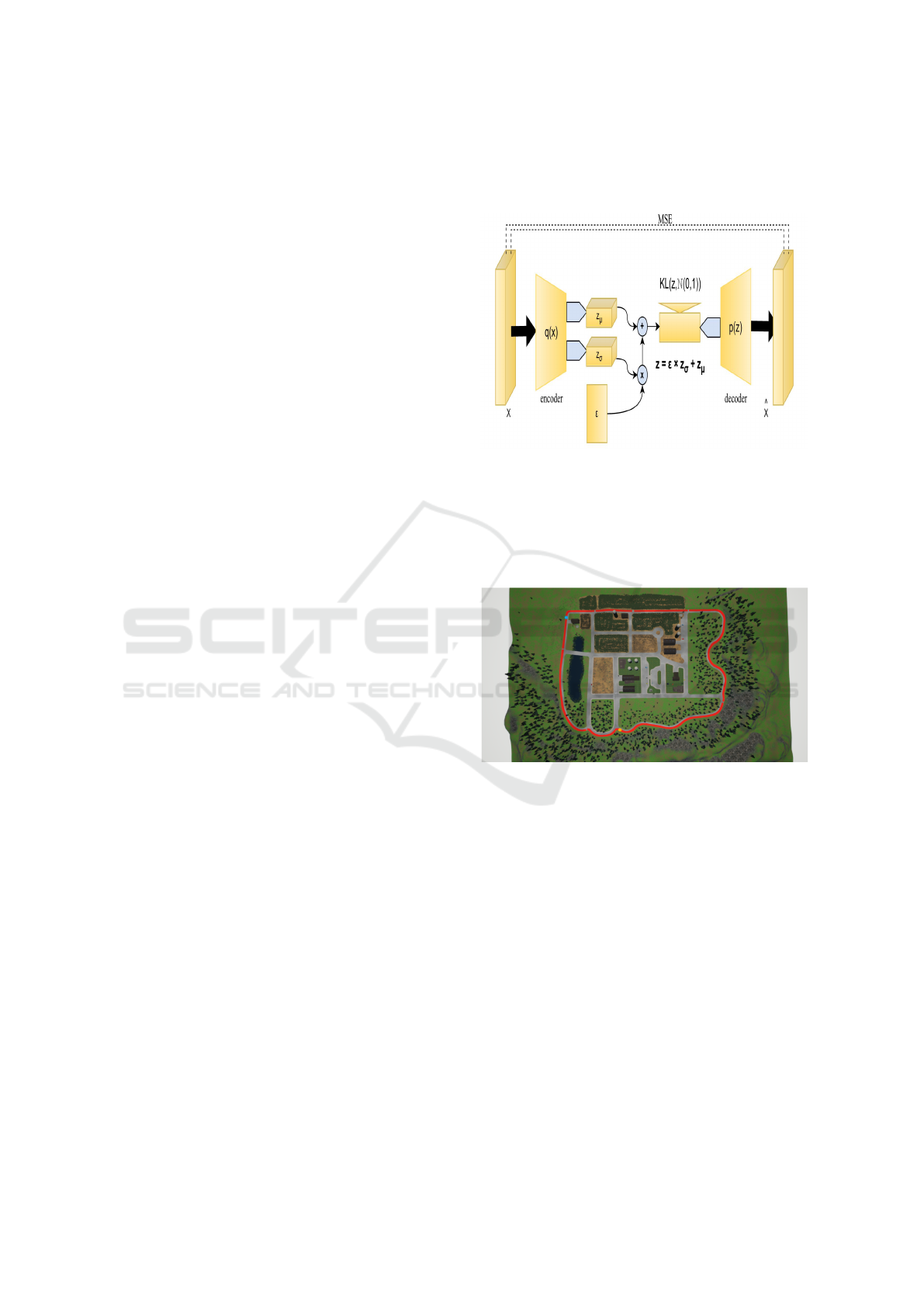
Figure 1: Variational autoencoder architecture.

Figure (1) shows a variational autoencoder archi-

tecture. The encoder operates on the input vector,

yielding two vectors, z

and z

. Then, a sample z

is drawn from the distribution N(z

), which is fed

into the decoder p, producing a reconstructed signal.

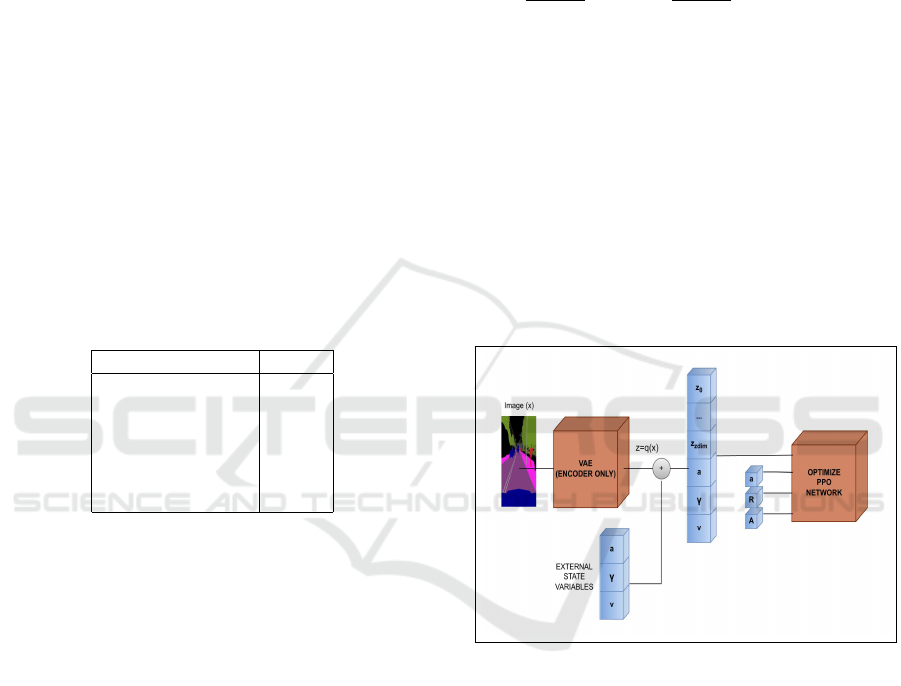
Figure 2: Top down view of the lap in Town 7.

3 EXPERIMENTAL STUDY AND

RESULT ANALYSIS

In this section, we present the experimental setup,

methodology, and results of our study. We start by de-

scribing the experimental environment, followed by a

detailed explanation of the evaluation metrics and the

baseline methods for comparison. We then present

the results of our experiments and ﬁnally discuss the

implications of our ﬁndings and compare our results

with existing work in the ﬁeld.

CuRLA: Curriculum Learning Based Deep Reinforcement Learning for Autonomous Driving

437

3.1 Proposed Model and Experimental

Study

Our model is named as CuRLA and the model used

in the base paper is named as Self-Centering Agent

(SCA) for further reference. We also perform exper-

iments using only curriculum learning for the opti-

mized reward function to compare it’s performance to

the two-fold curriculum learning method that is im-

plemented in CuRLA. This model is named One-Fold

CL. We use Town 7 from the list of Towns in CARLA

Lap Environment (Dosovitskiy et al., 2017) as shown

in ﬁgure (2). The reason for using this speciﬁc town

is that it provides a highway environment without any

exits, thus making our job of end-to-end driving eas-

ier. In our experiments, curriculum learning is em-

ployed by gradually increasing trafﬁc volume and in-

troducing functionalities to the agent in it’s reward

function in stages, allowing it to quickly grasp the

basics of the environment and efﬁciently tackle more

complex tasks.

Table 1: VAE Parameters.

Hyperparameter Value

dim

Architecture CNN

Learning rate α 1e − 4

β 1

Batch size N 100

Loss BCE

The VAE (Kingma and Welling, 2022) we

have used serves as feature extractors by com-

pressing high-dimensional observations into a lower-

dimensional latent space. This aids the learning pro-

cess by providing a more manageable representation

for the agent. Variational Autoencoder (VAE) is cho-

sen as it is used for learning probabilistic representa-

tions of the input in the latent space, unlike regular

autoencoders (Rumelhart et al., 1986), which learn

deterministic representations. We use the VAE archi-

tecture from (Vergara, 2019) to encode the state of

the environment, utilizing the pre-trained VAE from

the same study to replicate the encodings. The dataset

used to train the VAE contains 9000 training and 1000

validation examples (total of 10,000 160 × 80 RGB

images), all collected manually from the driving sim-

ulator environment.

We have made use of the state-of-the-art PPO-

Clip (Schulman et al., 2017b) algorithm to optimize

our agent’s policy and to arrive at an optimal policy

that maximizes the return. PPO-Clip clips the pol-

icy to ensure that the new policy does not diverge far

away from the old policy. The policy update equation

of PPO-Clip is given as:

k+1

= argmax

s,a∼θ

[L(s,a,θ

,θ)] (1)

Here, L is given as:

L(s,a,θ

,θ) =

min



(a|s)

,clip



(a|s)

,1 + ε,1 − ε



(2)

Here, θ refers to the policy parameters being up-

dated, and θ

is the policy parameters currently being

used in the k

iteration to get the next iterations pa-

rameters, θ

k+1

. Also, ε is the clipping hyperparameter

deﬁning how much the new policy can diverge from

the old one. The min in the objective computes the

minimum of the un-clipped and clipped objectives.

The overall graphical representation of the

PPO+VAE training process we have used in our pa-

per is shown in the ﬁgure (3).In the ﬁgure (3), the ex-

ternal variables are acceleration, steering angle, and

speed from top to bottom.

Figure 3: PPO+VAE training architecture.

The models are trained with the same parameters

mentioned in (Vergara, 2019). Table 2 shows the

complete list of hyperparameters used in the experi-

ments. All models are trained for 3500 episodes, and

the evaluation is done once every 10 episodes. Cur-

riculum learning is implemented in both CuRLA and

One-Fold CL. After 1500 episodes, trafﬁc and a col-

lision penalty are introduced in CuRLA. In One-Fold

CL, only the collision penalty is introduced after 1500

episodes, and trafﬁc is present from the ﬁrst episode

itself. An episode ends when the agent ﬁnishes three

laps, drifts off the center of the lane by more than 3

metres, or has a speed of less than 1 km/hr for 5 sec-

onds or more. A collision will not lead to the end of

an episode (unless the agent collides and maintains a

low speed under 1 km/hr for 5 seconds and more due

ICAART 2025 - 17th International Conference on Agents and Artiﬁcial Intelligence

438

to the collision). The results we obtain are shown in

Figs [6,8,7,9].

Table 2: Model Parameters.

Hyperparameters Value

Batch size M 32

Entropy loss scale β 0.01

GAE parameter λ 0.95

Initial noise σ

init

0.4

Epochs K 3

Discount γ 0.99

Value loss scale α 1.0

Learning rate 1e − 4

PPO-Clip parameter ε 0.2

Horizon T 128

3.2 Improvements Made

3.2.1 Reward Function Optimization

Keeping the architecture of the VAE and the RL al-

gorithm the same as the original paper, we chose to

change the original reward function. The original re-

ward function (3) has 3 components: the angle reward,

the centering reward, and the speed reward. Our re-

vised reward function (4) has 4 components, the three

original components, and we have also added a col-

lision penalty, to encourage the agent against unsafe

driving behaviour.

r = r

· r

(3)

′

= r

· r

′

+ r

(4)

1. Angle Reward: The angle reward component en-

sures that the agent is aligned with the road. An-

gle α, determines the angle difference between the

forward vector of the vehicle (the direction the

vehicle is heading in) and the forward vector of

the vehicle waypoint (the direction the waypoint

is aligned with). Using α, the angle reward r

deﬁned by

= max



1 −



max





(5)

where α

max

= 20

◦

(π/9 radians).

This ensures that the angle reward r

∈ [0,1], and

that the angle reward linearly decreases from 1

(perfect alignment) to 0 (when the deviation is 20

◦

or more).

2. Centering Reward. The centering reward factor

ensures that the driving agent stays to the center

of the lane. The usage of a high-ﬁdelity simulator

like CARLA enables us to have a precise mea-

surement of distance between objects in the envi-

ronment. To reward the agent for staying within

the center of the lane, we use the distance d be-

tween the center of the car and the center of the

lane to deﬁne the centering reward by



1 −

max



(6)

where d

max

= 3.

This ensures that the centering reward component

∈ [0, 1] (as the episode terminates when the

agent goes off center by more than 3 metres) and

that r

is inversely proportional to d, encouraging

more centering for the agent while driving.

3. Speed Reward. While keeping the angle and

centering reward the same for all three agents,

we change the speed reward component. The

minimum speed v

min

, maximum speed v

max

, and

target speed v

target

are taken as 15 Km/hr, 105

Km/hr and 60 Km/hr respectively, and are kept as

the same for both the original and updated speed

reward components. The original speed reward

component r

and the new speed reward compo-

nent r

′

are then deﬁned by











min

, v < v

min

1, v

min

≤ v ≤ v

target

1 −

v−v

target

max

−v

target

, v

target

< v ≤ v

max

(7)

′











0.5 ·

min

, v < v

min

1 −

target

−v

target

−v

min

, v

min

≤ v ≤ v

target

max

−v

max

−v

target

, v

target

< v ≤ v

max

(8)

where v is the current speed of the agent.

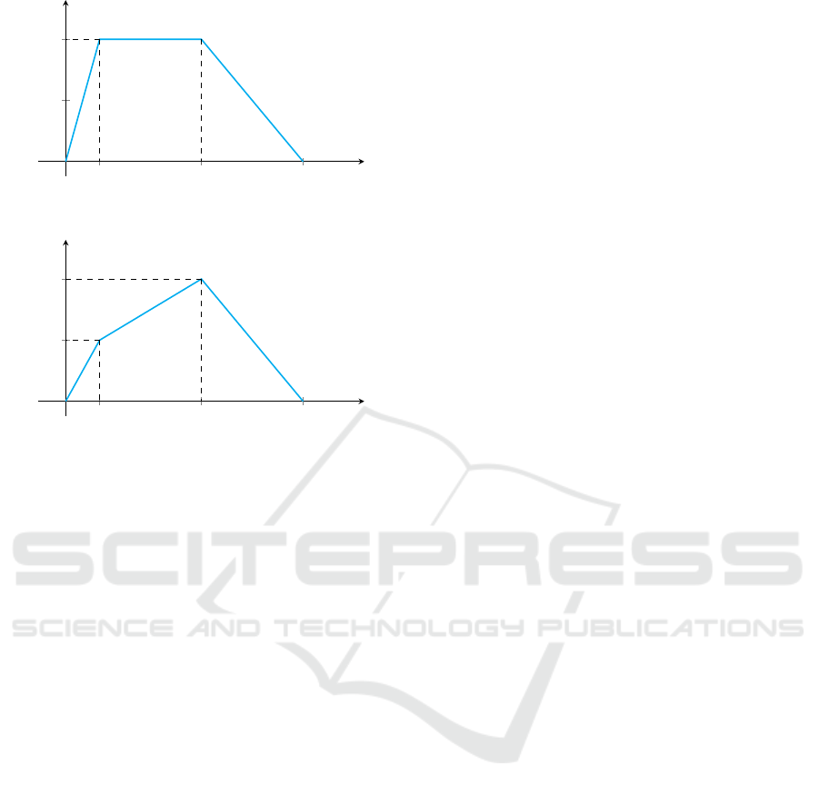
As seen in the graphs (Fig.4 & Fig.5), in the orig-

inal speed reward function (Fig.4), the graph is

constant in the range [v

min

, v

target

] and receives

the highest reward of 1. This is misleading as

the agent can get confused, deciphering the mini-

mum speed as the target speed itself, as it is get-

ting a constant reward of 1 at either speed. This

ensures that the agent will drive slower, as ensur-

ing a higher centering and angle reward at a lower

speed is much easier than at a higher speed. To

rectify this, we have replaced the constant graph

in [v

min

, v

target

] with an increasing function (see

Fig.5) to prioritize getting as close to the target

speed as possible without losing too much perfor-

mance on the angle and centering reward compo-

nents. Both CuRLA and One-Fold CL use this

revised reward function, whereas SCA uses the

original reward function.

4. Collision Penalty. A collision penalty factor was

introduced for both One-Fold CL and CuRLA to

CuRLA: Curriculum Learning Based Deep Reinforcement Learning for Autonomous Driving

439

15 60 105

0.5

Speed

Reward

Figure 4: SCA Reward Function.

15 60 105

0.5

Speed

Reward

Figure 5: CuRLA & One-Fold CL Reward Function.

ensure the agent explicitly learns the behaviour of

safe driving, avoiding collisions with other objects

and vehicles in the environment. The advantage

of using a simulator like CARLA also enables us

to get a collision intensity (I

) value between the

agent and other objects in the environment, which

we use to devise the collision penalty. The colli-

sion penalty r

is deﬁned by

= max(−1,−log

(max(1,I

))) (9)

This penalty ensures r

∈ [−1,0], thus ensuring

′

∈ [−1,1].

3.2.2 Curriculum Learning

In CuRLA, curriculum learning is implemented in a

two-fold manner. Firstly, we gradually increase the

trafﬁc volume of our simulation environment as the

number of episodes increases. The agent gets to fo-

cus on learning to drive in a trafﬁc-free environment

initially and then slowly navigate through trafﬁc in

the later epochs. Secondly, the functionalities of the

agent are gradually added. As the agent learns to drive

in a trafﬁc-free environment, we introduce a collision

penalty while increasing the volume of trafﬁc to teach

it to avoid collisions with other vehicles. The reason-

ing behind adding this collision penalty is that while

the current reward function accounts for smooth driv-

ing, it does not punish the agent enough for colliding

with the other vehicles. All agents have been trained

with trafﬁc included in the roads, making a collision

penalty extremely important. This method of training

helped the agent to learn the basics of the environment

quickly and enabled it to learn harder tasks efﬁciently

while also keeping safety as a factor.

3.3 Metrics and Result Analysis

The models are compared on two metrics - distance

travelled and average speed. These metrics are cho-

sen as they capture an accurate representation of the

trade-off between efﬁciency and performance in au-

tonomous driving scenarios. The distance traveled

metric emphasizes the model’s capability to maxi-

mize the length of the path it traverses, reﬂecting

its ability to sustain long journeys without interrup-

tion. Conversely, the average speed metric accounts

for both the distance covered and the time taken to

complete the journey, offering a thorough assessment

of the model’s performance in terms of both speed

and efﬁciency. Evaluating these metrics provides a

detailed understanding of how each model balances

speed and distance, which are essential factors in as-

sessing the overall effectiveness of autonomous driv-

ing systems. The evaluation of our models against

the base model provided insightful ﬁndings. (All

graphs have been considered with a smoothing factor

of 0.999)

In our assessment, for the metric of Distance Trav-

eled, we measure it by the number of laps traveled by

the vehicle, where 100% is considered as one lap ﬁn-

ished. As it can be seen in Fig.6 & Fig.7, CuRLA

and SCA have similar performance, completing ap-

proximately 1.5 laps on average in training and 0.3

laps in evaluation. Meanwhile, One-Fold CL did

worse than both CuRLA and SCA, completing ap-

proximately 1.25 laps in training and 0.25 laps in eval-

uation. CuRLA does perform slightly better in train-

ing compared to SCA, which performs slightly better

in evaluation. However, from the graph it can be seen

that CuRLA had a consistent learning curve while

training compared to SCA, which dropped in perfor-

mance and then picked back up. One-Fold CL also

performed comparably to both models, albeit slightly

worse. This attests to the improvement in perfor-

mance that two-fold curriculum learning shows over

simple curriculum learning during training and train-

ing without curriculum learning.

The assessment of the metric of Average Speed

highlighted the strengths of our assumption in chang-

ing the underlying speed reward component. During

training, as can be seen in Fig.8, both CuRLA and

One-Fold CL signiﬁcantly outperform SCA reaching

average speeds of 22 Km/hr and 20 Km/hr in train-

ing, compared to SCA’s 14 Km/hr. The difference is

ICAART 2025 - 17th International Conference on Agents and Artiﬁcial Intelligence

440

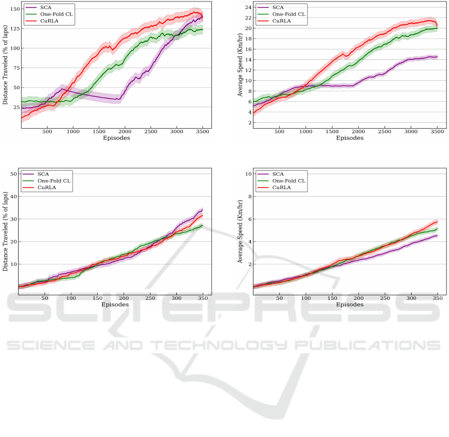
Figure 6: Training Metric: Distance Traveled.

Figure 7: Evaluation Metric: Distance Traveled.

not as much during evaluation (Fig.9), but CurLA and

One-Fold CL still outperform SCA here as well, with

CuRLA reaching an average speed of 6 Km/hr and

One-Fold CL reaching an average speed of 5 Km/hr,

compared to SCA’s 4 Km/hr. This superior perfor-

mance of CuRLA and One-Fold CL (on the revised

reward function) compared to the SCA agent (using

the original reward function) underscores our reward

function’s efﬁciency in optimizing speed-related as-

pects.

4 CONCLUSIONS

In this paper, we presented a model (CuRLA) that

used a PPO+VAE architecture and two-fold curricu-

lum learning along with a reward function tuned to

accelerate the training process and achieve higher av-

erage speeds in autonomous driving scenarios. We

show the performance of two-fold curriculum learn-

ing against simple curriculum learning (One-Fold CL

agent), as well as the performance of agents on the

revised reward function compared to the base reward

function. While CuRLA and One-Fold CL perform

comparably to the base agent (SCA) in the distance

Figure 8: Training Metric: Average Speed.

Figure 9: Evaluation Metric: Average Speed.

traveled metric (with CuRLA performing slightly bet-

ter and One-Fold CL being slightly worse), a sig-

niﬁcant improvement in average speed is observed.

This prioritization of speed was a deliberate design

choice. The distance traveled metric solely opti-

mizes for maximizing the traversed path length. Con-

versely, the average speed metric inherently optimizes

for both distance and the time taken to complete the

journey, effectively accounting for two performance

factors within a single measure. The performance of

CuRLA and One-Fold CL agents, when compared to

SCA, also attest to the beneﬁts of using curriculum

learning while training, and how decomposing the

tasks in the autonomous driving problem helps agents

to learn better and faster. Integrating multiple objec-

tives into a single scalar reward function often leads

to suboptimal agent performance. However, by em-

ploying curriculum learning during training, we can

enable agents to master the nuances of each reward

component more effectively. This approach facilitates

better understanding of the environment and objec-

tives, and ultimately enhances overall performance.

Future research will focus on enhancing perfor-

mance by updating the architecture and algorithms.

One area of interest is investigating vision-based

CuRLA: Curriculum Learning Based Deep Reinforcement Learning for Autonomous Driving

441

transformers and advanced transformer-based rein-

forcement learning methods for autonomous driv-

ing control. This entails replacing the current Vari-

ational Autoencoder with architectures like Vision

Transformers (ViT, Swin Transformer, ConvNeXT)

tailored for raw visual data. Furthermore, newer

techniques such as Decision Transformers or Trajec-

tory Transformers could replace the Proximal Policy

Optimization (PPO) algorithm to potentially enhance

decision-making capabilities. Another promising area

for future research is Multi-Objective Reinforcement

Learning (MORL) (Van Moffaert and Now

e, 2014;

Hayes et al., 2021; Liu et al., 2015), where an agent

optimizes multiple reward functions, each represent-

ing different objectives. Evaluating these advance-

ments through simulated testing may lead to substan-

tial performance improvements.

REFERENCES

Baldi, P. (2011). Autoencoders, unsupervised learning, and

deep architectures. In ICML Unsupervised and Trans-

fer Learning.

Bengio, Y., Louradour, J., Collobert, R., and Weston, J.

(2009). Curriculum learning. volume 60, page 6.

Dickmanns, E. D. and Zapp, B. (1987). An integrated dy-

namic scene analysis system for autonomous road ve-

hicles. In Intelligent Vehicles ’87, pages 157–164.

IEEE.

Dosovitskiy, A., Ros, G., Codevilla, F., Lopez, A., and

Koltun, V. (2017). Carla: An open urban driving sim-

ulator.

Grigorescu, S., Trasnea, B., Cocias, T., and Macesanu,

G. (2019). A survey of deep learning techniques

for autonomous driving. Journal of Field Robotics,

37(3):362–386.

Hayes, C. F., Radulescu, R., Bargiacchi, E., K

allstr

om,

J., Macfarlane, M., Reymond, M., Verstraeten, T.,

Zintgraf, L. M., Dazeley, R., Heintz, F., Howley,

E., Irissappane, A. A., Mannion, P., Now

e, A.,

de Oliveira Ramos, G., Restelli, M., Vamplew, P., and

Roijers, D. M. (2021). A practical guide to multi-

objective reinforcement learning and planning. CoRR,

abs/2103.09568.

Kendall, A., Hawke, J., Janz, D., Mazur, P., Reda, D., Allen,

J.-M., Lam, V.-D., Bewley, A., and Shah, A. (2018).

Learning to drive in a day.

Kingma, D. P. and Welling, M. (2022). Auto-encoding vari-

ational bayes.

Krizhevsky, A., Sutskever, I., and Hinton, G. (2012). Im-

agenet classiﬁcation with deep convolutional neural

networks. Neural Information Processing Systems,

25.

Kullback, S. and Leibler, R. A. (1951). On information

and sufﬁciency. The Annals of Mathematical Statis-

tics, 22(1):79–86.

Li, Y. and Ibanez-Guzman, J. (2020). Lidar for autonomous

driving: The principles, challenges, and trends for au-

tomotive lidar and perception systems. IEEE Signal

Processing Magazine, 37(4):50–61.

Lillicrap, T. P., Hunt, J. J., Pritzel, A., Heess, N., Erez, T.,

Tassa, Y., Silver, D., and Wierstra, D. (2019). Contin-

uous control with deep reinforcement learning.

Liu, C., Xu, X., and Hu, D. (2015). Multiobjective rein-

forcement learning: A comprehensive overview. IEEE

Transactions on Systems, Man, and Cybernetics: Sys-

tems, 45(3):385–398.

Mnih, V., Badia, A. P., Mirza, M., Graves, A., Lillicrap,

T. P., Harley, T., Silver, D., and Kavukcuoglu, K.

(2016). Asynchronous methods for deep reinforce-

ment learning.

Mnih, V., Kavukcuoglu, K., Silver, D., Graves, A.,

Antonoglou, I., Wierstra, D., and Riedmiller, M.

(2013). Playing atari with deep reinforcement learn-

ing.

Moravec, H. (1990). Sensor fusion in autonomous vehicles.

In Sensor Fusion, pages 125–153. Springer, Boston,

MA.

Narvekar, S., Peng, B., Leonetti, M., Sinapov, J., Taylor,

M. E., and Stone, P. (2020). Curriculum learning for

reinforcement learning domains: A framework and

survey.

Pomerleau, D. A. (1988). Alvinn: An autonomous land

vehicle in a neural network. In Touretzky, D., editor,

Advances in Neural Information Processing Systems,

volume 1. Morgan-Kaufmann.

Rumelhart, D. E., Hinton, G. E., and Williams, R. J. (1986).

Learning internal representations by error propaga-

tion.

Schulman, J., Levine, S., Moritz, P., Jordan, M. I., and

Abbeel, P. (2017a). Trust region policy optimization.

Schulman, J., Wolski, F., Dhariwal, P., Radford, A., and

Klimov, O. (2017b). Proximal policy optimization al-

gorithms.

Sutton, R. S., McAllester, D., Singh, S., and Mansour, Y.

(1999). Policy gradient methods for reinforcement

learning with function approximation. In Solla, S.,

Leen, T., and M

uller, K., editors, Advances in Neu-

ral Information Processing Systems, volume 12. MIT

Press.

Thrun, S., Burgard, W., and Fox, D. (2005). Probabilis-

tic Robotics (Intelligent Robotics and Autonomous

Agents).

Van Moffaert, K. and Now

e, A. (2014). Multi-objective re-

inforcement learning using sets of pareto dominating

policies. The Journal of Machine Learning Research,

15(1):3483–3512.

Vergara, M. L. (2019). Accelerating training of deep rein-

forcement learning-based autonomous driving agents

through comparative study of agent and environment

designs. Master thesis, NTNU.

Wikipedia contributors (2024). Darpa grand challenge

(2005) — Wikipedia, the free encyclopedia.

ICAART 2025 - 17th International Conference on Agents and Artiﬁcial Intelligence

442