Lightweight Visualisation for Vortex Tracking in Airflow Acquisition
Nicolas Courilleau
1 a
, Louis-Wilhelm Raban-Schürmann
1 b
, Daniel Meneveaux
1 c
,
Kamel Abed-Meraim
2
and Anas Sakout
2 d
1
Université de Poitiers, XLIM Institute, CNRS UMR 7252, France
2
Université de La Rochelle, LaSIE, CNRS UMR 7356, France
Keywords:
Visualisation of Airflow, Rendering, Vortex Analysis, Flow Tracking.
Abstract:
Ventilation systems are spread in most buildings and housing. They provide control on air quality, while pro-
visioning acceptable thermal conditions. However, slotted plates that direct air jets often produce acoustic
disturbances with a self-sustained tone. Understanding and controlling the phenomenon requires complex
experimentation with expensive setups. This article proposes an open source, web-based, interactive visuali-
sation system dedicated to the observation and analysis of recorded high frequency captures (3kHz or more)
of air streams, charged with thin oil particles. It relies on the acquired images and estimated vector fields,
coming from industrial existing systems. Our goal is to visualise the main flow parameters, such as speed, gra-
dients, directions, vortex tracking with path prediction, and vortex frequencies. The obtained results highlight
interesting phenomena that illustrate sounds production. They can be employed by physicists to understand,
explain, and control the generated acoustics.
1 INTRODUCTION
Airflow control in the industry is widely employed in
various contexts such as air conditioning systems, or
wind tunnel operations for instance. Unfortunately,
the geometric shape of flap systems creates distur-
bances that often result in undesirable acoustic phe-
nomena, such as whistling or humming. With some
configurations, oscillating patterns appear and inten-
sify noise. Countermeasures can be considered, based
on flat shapes or flow manipulators. However, setting
up an experimental system is costly, requires a rigor-
ously controlled environment, and involves extensive
testing.
For these reasons, several authors have conducted
comprehensive studies on plane jets with obstacles
using PIV (Particle image velocimetry) techniques
(Gutmark et al., 1978; Sakakibara et al., 2001). For
instance, it has been determined that the detachment
frequency of vortex rollers in a plane jet is influenced
by the jet’s initial conditions (Yokobori et al., 1983).
a
https://orcid.org/0000-0001-7707-9288
b
https://orcid.org/0009-0001-5010-7397
c
https://orcid.org/0000-0001-7160-3026
d
https://orcid.org/0000-0003-2571-5531
Filaments identified in the contra-rotating vortex zone
persist in the stagnation zone and continue moving in
the longitudinal direction, playing a key role in the in-
teraction with wall flows (Gutmark et al., 1978). Fur-
thermore, the counter-rotating filaments on either side
of the jet’s symmetry plane merge at the obstacle to
form longitudinal rollers that cross this plane (Sakak-
ibara et al., 2001).
This article proposes an open lightweight tool for
airflow visualisation of PIV acquired data, only re-
quiring a web browser. It aims at providing efficient
particle and vortex tracking, displaying vortex cen-
ters and trajectories. More importantly, it estimates
the vortex formation frequency, based on the captured
image flow. Our contributions proposed in this article
are the following:
 A lightweight tool for analysing air flow images;
 A velocity vector fields visualisation;
 A particle tracking system, with trajectories;
 A vortex tracking method, highlighting intensities
and directions;
 A vortex apparition detection, related to the
acoustic frequency.
In this paper, the visualisation system focuses on
plane jets impinging on a slotted plate.
Courilleau, N., Raban-Schürmann, L.-W., Meneveaux, D., Abed-Meraim, K. and Sakout, A.
Lightweight Visualisation for Vortex Tracking in Airflow Acquisition.
DOI: 10.5220/0013147400003912
Paper published under CC license (CC BY-NC-ND 4.0)
In Proceedings of the 20th International Joint Conference on Computer Vision, Imaging and Computer Graphics Theory and Applications (VISIGRAPP 2025) - Volume 1: GRAPP, HUCAPP
and IVAPP, pages 223-230
ISBN: 978-989-758-728-3; ISSN: 2184-4321
Proceedings Copyright © 2025 by SCITEPRESS – Science and Technology Publications, Lda.
223

2 RELATED WORK
Visualising an airflow is particularly challenging
since air is transparent to the naked eye. Alternative
methods must be employed to highlight the flow pat-
terns. Furthermore, the targeted phenomena often oc-
cur at high frequencies, difficult to capture or analyse
in real time. Therefore, both high-speed visualisa-
tion techniques and advanced post-processing meth-
ods have to be implemented.
In many cases, PIV is used to track the movement
of particles suspended in the air, allowing researchers
to indirectly observe airflow behavior. Many tools al-
ready exist to visualise such complex data sets (Dorier
et al., 2013; Ayachit et al., 2016; Sarton et al., 2023).
Two major communities have formed around two key
tools: ParaView (Ahrens et al., 2005; Ayachit et al.,
2015) and VisIt (Kuhlen et al., 2011; Childs et al.,
2012). They have been specifically designed for
large-scale data visualisation, particularly well-suited
for simulations. Despite their strengths, they are not
versatile enough to accommodate experimental data
provided by specific hardware.
Consequently, physicists often turn to commercial
tools like DaVIS from LaVision, which are specif-
ically tailored to handle experimental data (DaVIS,
2024). These tools are by design compatible with the
associated hardware. However, in addition to their
high cost, they are proprietary software, making adap-
tions to specific functionalities impossible.
As a result, many laboratories prefer to rely on
custom-built solutions to process their data. They of-
ten use tools such as MATLAB, Octave, or Tecplot,
for instance. The primary advantage of these solu-
tions is that they allow complete control over the fea-
tures developed, ensuring that the tools are tailored
to meet the specific needs of physicists. However, the
downside is that physicists may lack the programming
expertise to develop fully optimised tools, leading to
inefficiencies.
3 EXPERIMENTAL PLATFORM
When a plane jet reaches an obstacle, it produces an
audible acoustic shock wave, that may interact with
the plane jet, creating a self-sustained acoustic phe-
nomenon. It is similar to the sound produced with
wind instruments or to the howling wind in canyons
for instance.
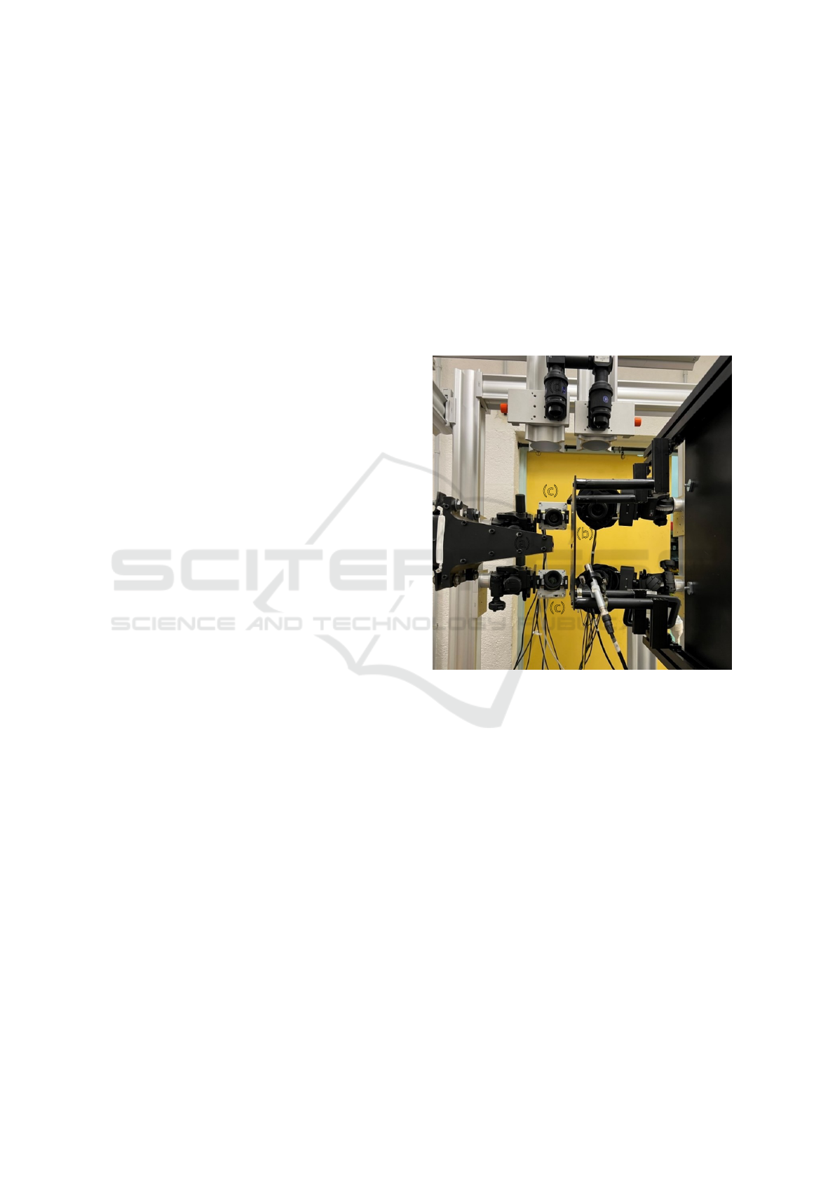
This article relies on an existing experimental
setup that contains five main elements for studying air
flows: a blowing system, an thin oil particles seeding
system, a laser beam, a high frequency camera, and
an acoustic system. A full acquisition cycle can re-
quire up to a month of preparation for capturing one
second of data. Figure 1 shows a photograph of the
acquisition part of this setup.
Fluid flow patterns depend on various parameters,
such as fluid viscosity, density, flow speed, and the
geometric configuration of the medium. They are
characterised by the Reynolds number (Re) (Som-
merfeld, 1909; Bush, 2004). This value is thus fun-
damental when designing an experimental setup. A
low Reynolds number corresponds to a laminar flow,
while a high Reynolds number is related to a turbulent
flow.
(a)
(d)
(c)
(b)
(e)
(c)
Figure 1: Photograph of the experimentation setup: (a) con-
vergent nozzle, (b) slotted plate, (c) high-frequency cam-
eras, (d) laser emitter, and (e) microphone.
Blowing System
First, the blowing system controls the flow velocity,
directed toward a slotted plate. It comprises three el-
ements:
1. A compressor and frequency chopper (Figure 2.a),
located in an isolated room, that produces airflow
while avoiding interference with acoustic phe-
nomena from the impinging jet. A digital fre-
quency chopper manages the motor frequency,
controlling the jet’s initial speed, which can reach
33 m/s (subsonic).
2. A 1m
3
damping chamber and a tube with a con-
vergent nozzle. It is equipped with three coarse
metal meshes, reducing turbulence. The 1250 mm
long rectangular tube (190 mm × 90 mm), fitted
with honeycomb structures and a convergent noz-
GRAPP 2025 - 20th International Conference on Computer Graphics Theory and Applications
224

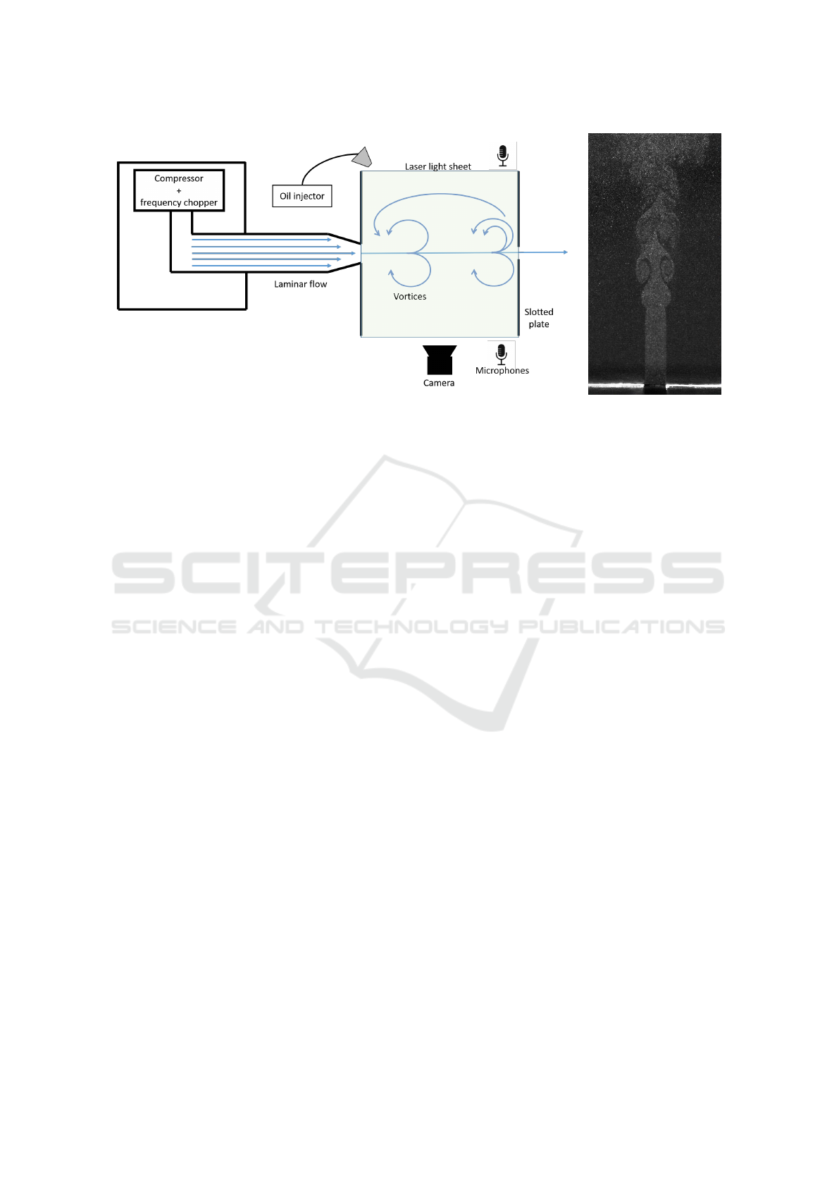
(a) (b)
Figure 2: (a) Representation of the experimentation setup. On the left the compressor and frequency chopper generating the
airflow outside of the experimentation room. In the middle the laminar flow. On the right the acquisition part. Oil particles
are injected in the air flow and a high-frequency camera capture the response a of the light bouncing on the particles from a
laser sheet. Finally, microphones captures the acoustic spectrum. (b) Raw Image produced for a free plane jet without any
obstacle.
zle, produces a plane jet of height H=10 mm and
width 190 mm, achieving an aspect ratio of 19.
This ensures a laminar jet at the nozzle exit with
minimal turbulence (Assoum et al., 2020).
3. An obstacle, corresponding to a 4 mm thick alu-
minum plate with a 45° beveled slot aligned to the
nozzle outlet. Acoustic resonance occurs upon
impact, and Reynolds number adjustments are
controlled here. Image and acoustic acquisition
are performed in this final element.
Image Acquisition
The fluid flow is seeded by thin oil particles, illu-
minated by a high-intensity pulse laser beam with
short duration. The acquisition technique consists in
capturing the resulting images at high frequency (at
3KHz for this article). The oil particles must be small
enough to follow velocity gradients but large enough
to scatter sufficient light, in order to minimize noise
during processing. Seeding must be performed care-
fully, upstream from the measurement volume, for
avoiding disturbances. Note that PIV measures par-
ticle velocity rather than exact flow velocity. For our
experimentation, the camera is placed orthogonally to
the laser plane. Synchronization and calibration en-
sure accurate data acquisition.
The system also includes an acoustic acquisition
system, simultaneously with the image acquisition.
10 KHz Microphones are placed on each side of the
experimentation setup capture the full acoustic spec-
trum. This article focuses on the visualisation system,
links between vortex analysis and acoustic effects will
be considered in future work.
4 FLOW TRACKING
Studying the sound generated by a blowing system
requires understanding the flow dynamics, and more
specifically vortex formation. This is why we propose
a tool for visualising air flow motion with its char-
acteristics such as speed, transverse and longitudinal
velocities, or vortex formation and motion. Our visu-
alisation system uses as input the series of acquired
images, each associated with its corresponding veloc-
ity vector field (Figure 2.b).
Input Data Direct Visualisation
Flow vectors are given as a set of 2D points aligned
with a uniform grid in image space. Aligning these
points with the acquired image at each time step al-
lows for visualising raw data, with 3 modes: individ-
ual, transverse, and longitudinal velocities (Figure 3).
A user-chosen colormap helps to visually identify re-
gions of low or high velocities:
 The individual velocity mode (Figure 3.a) em-
ploys a mapping of the velocity vector norm, aid-
ing shear flow analysis;
 The transverse mode (Figure 3.b) isolates the x-
component of velocity, showing the extent of lat-
eral motion;
Lightweight Visualisation for Vortex Tracking in Airflow Acquisition
225

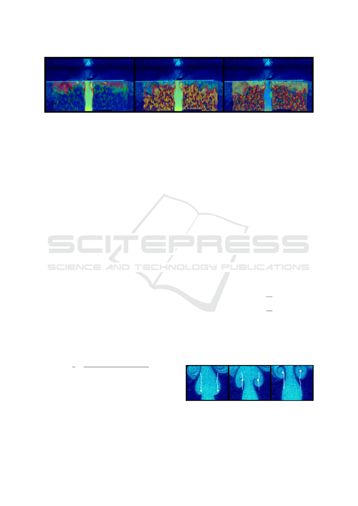
a
b
c
Figure 3: Visualisation of the vector fields, (a) individual velocity, (b) transverse velocity, and (c) longitudinal velocity, on top
of the corresponding frame captured. Vector magnitudes are normalized and mapped on a predefined spectrum, that represents
magnitudes: blue for low speed, green for intermediate, red for high, and yellow for the highest.
 The longitudinal mode (Figure 3.c) isolates the y-
component of velocity, representing vertical mo-
tion, also highlighting upstream or downstream
dynamics, useful for identifying rising or de-
scending vortices.
Vortex Detection
Tracking vortexes can be managed using the Gamma
2 (Γ
2
) criterion, proposed by (Graftieaux et al., 2001).
It has successfully been employed for identifying vor-
tices in turbulent flows. This approach differentiates
between rotational and shear flows by integrating the
local velocity field over a small domain. In rotation-
dominated flows, particles move around a common
center in a circular or spiral manner, indicating re-
gions where the velocity field characterises coherent,
organised rotational motion. The corresponding re-
gions are referred to as vortices. Vortices are areas
where fluid elements exhibit significant vorticity, a
measure of the local rotation of fluid particles. In con-
trast, shear flows occur when fluid layers move paral-
lel to each other at different velocities. In this case,
no significant rotational movement of fluid elements
occurs.
Γ
2
computations correspond to iterating through
flow data and estimating vortex structures. They are
later used to generate texture maps of vortex cores.
The method mirrors the theoretical Γ
2
formulation,
accurately distinguishing vortex cores from regions
dominated by shear. Mathematically, Γ
2
expression
at a point P is:
Γ
2
=
1
S
Z
S
−→
PM × (
−→
u (M) −
−→
u (P))·
−→
z
|
−→
PM|
2
dS,
where S is the surrounding domain,
−→
PM is the vec-
tor from P to a neighbouring point M, and
−→
u (M)
and
−→
u (P) represent the velocities at M and P.
−→
z is
the unit normal vector to the observation plane. This
computation highlights rotational flow regions, iden-
tifying vortices even in noisy environments.
In their work, (Graftieaux et al., 2001) compares
two integration domains, square and circular, applied
to the Γ
2
criterion. The conclusion is that circular
domains generally offer better accuracy in detecting
vortex cores by preserving the symmetry of the struc-
tures, while square domains, aligned with the Carte-
sian frame, simplify calculations and improve com-
putational efficiency. In this implementation it makes
more sense to use a square domain, as a core objective
is to propose a visualisation at an interactive frame
rate.
Vortex Trajectory Calculation
Proposing a viable vortex visualisation involves to
recreate time coherence between the defined vortices
throughout the source samples. Therefore, it tracks
vortex trajectories by following particle movements
through the flow field. The tracking is done by updat-
ing velocities and positions using bilinear interpola-
tion.
At each time step, it computes particle velocities
from the surrounding four grid points. The position
update is computed as follows:
x
new
= x
current
+
v
x
K
v
y
new
= y
current
+
v
y
K
v
where v
x
and v
y
are the interpolated velocity com-
ponents, K
v
is a user-defined value employed for ad-
justing the search radius (a value of 3.0 is suitable in
most cases). This step is repeated until the particle ei-
ther exits the flow domain or its velocity approaches
zero.
a
b
c
Figure 4: Vortex core trajectories and evolution of their po-
sitions over time.
Trajectories are computed at application start up
and stored in memory. An interpolation process pro-
GRAPP 2025 - 20th International Conference on Computer Graphics Theory and Applications
226

vides smoother approximations for each trajectory,
lowering the variations due to noisy input data. Fig-
ure 4 illustrates the trajectory calculated for one vor-
tex.
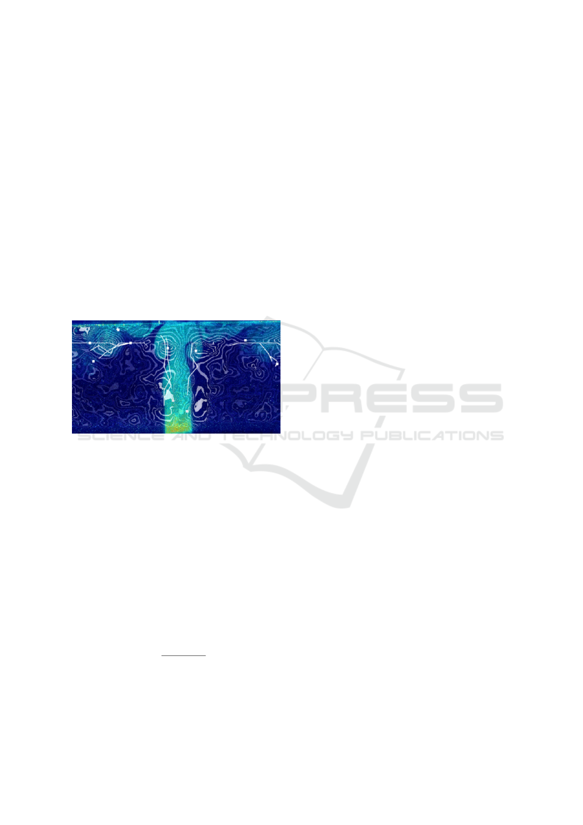
Wavefront Detection
We consider wavefronts as level sets, with scalar con-
tours used to highlight threshold values. Vortex in-
tensities (Γ
2
) are used as input values. They out-
line regions of interest, where particle angular veloc-
ity indicates high rotational intensity, enabling the vi-
sualisation and tracking of vortex structures and ve-
locity fronts in turbulent flows. They are integrated
as precomputed textures. Transparency and intensity
thresholds are dynamically adjustable, allowing flex-
ible rendering over vector fields or vortex trajecto-
ries. This multimodal approach clearly depicts vortex
boundaries by superposing level set contours on other
flow features (Figure 5).
Figure 5: Multimodal visualisation of a single frame,
present vortex cores with their trajectories and level set vi-
sualisation.
Vortex Frequency Calculation
Determining the frequency of vortex formation is also
an interesting parameter in understanding flow dy-
namics, notably when linked with sound generation.
For a given experimental setup, depending on the cho-
sen Re, the acoustic phenomenon is directly related to
the frequency of vortex formation. It is determined by
counting the number of vortex cores detected over a
series of frames.
The detection process relies on a rectangular
region selected by the user (ax, ay) and (bx, by),
mapped onto the data grid. The total number of de-
tected vortex occurrences n, is divided by the time in-
terval between frames, yielding the vortex frequency:
f =
n
∆t × ( j − i)
,
where ∆t is the time step between each frame of
the acquisition, and ( j − i) represents the number of
frames.
Implementation
The single most computationally expensive process
concerns level sets (Γ
2
). They are estimated in a
preprocessing step, written in python, integrating the
velocity field over localised regions and distributed
(multi-thread operations) to enhance performance.
This operation occurs only once per image series,
ensuring all essential data is completely available in
memory for real-time rendering.
Our real-time web-based tool relies on
javascript/webgl for the interactive visualisation
part. Adjusting vector colors for each mode is
ensured with vertex and fragment shaders, enabling
interactive visualisation of flow characteristics.
Vortex trajectories are calculated interactively at run
time, by tracking vortex cores across frames, from
the input velocity field.
The system supports multiple visualisation modes
(velocity, transverse, longitudinal), rendered in real-
time based on user input. Multimodal visualisation
allows users to switch between or combine modes dy-
namically, such as velocity fields, Γ
2
textures, and
level set contours.
Additionally, vortex frequency in a user-specified
region is calculated interactively by tracking vortex
occurrences over time, relying on precomputed data
and trajectory calculations.
5 RESULTS
Test System
Performance-wise, the tool was tested on a system
equipped with an Intel i5 processor, an RTX 2060 lap-
top GPU, and 16GB of RAM, making it accessible to
a broad audience with standard hardware. The tool
operates entirely within a web browser, specifically
Mozilla Firefox in our case, removing the need for
specialised software installations.
Test Data
The dataset used for testing consists of airflow data
captured over one second, with cameras recording at
3,000 frames per second, each dataset associated with
a specific Reynolds number (Figure 6). Each series of
acquisitions comprises 11GB of raw data and 8.9GB
of computed data prepared for visualisation, includ-
ing 3,000 images. Three datasets are presented in Fig-
ure 6 with an Reof 4700, 4800 and 5356 respectively.
Variations in Revisually corresponds to variations of
vortex core shapes and trajectories (note that higher
Redoes not necessarily imply higher vortex forma-
tion frequency). Our tool consistently delivers smooth
Lightweight Visualisation for Vortex Tracking in Airflow Acquisition
227

visualisation performance, with negligible impact on
the fluidity of the rendering process.
Figure 2.b shows input raw data examples, they
are grey-scale images associated with velocity vec-
tor fields. A look-up table enhances visualisation by
highlighting particles in the flow, as shown in Fig-
ure 3, 4, and 7.
Vector Fields Visualisation
The generated velocity vector fields are presented in
Figure 3. These vectors provide valuable insights
into both rotation-dominated and shear-dominated re-
gions. They reveal clear patterns of fluid rotation
around vortex cores, enabling the identification of
multiple vortices, their cores, and their trajectories, as
well as tracking their evolution over time.
Multimodal Visualisation
Figure 7.a shows the captured camera image along-
side the detected vortex cores in the current frame
and their trajectories. Figure 7.b presents the Γ
2
val-
ues derived from the corresponding velocity vector
field, providing a texture map that highlights regions
dominated by rotational motion, making the vortex
cores stand out more clearly. The colors represent
the Γ
2
values and indicate the direction of vortex
rotation, with saturated red and blue areas marking
regions of intense rotational activity, confirming the
presence of vortices while differentiating them from
shear-dominated regions.
Figure 5, in turn, displays the level set visualisa-
tion based on the Γ
2
values, showing the scalar field
of the flow and offering a qualitative measure of vor-
tex intensity or strength. The level set contours pro-
vide an additional layer of insight, delineating regions
of varying vortex intensity and tracking how these re-
gions evolve spatially across the flow domain, as de-
tailed in section 4. These contours also enable precise
identification of velocity fronts during visualisation.
Together, these three images illustrate the strength
of multimodal visualisation in fluid dynamics analy-
sis. The camera image, the Γ
2
texture, and the level
set, all together allow simultaneously observing the
structure, intensity, and trajectory of vortices within
the same simulation frame.
It is important to note that in multimodal visual-
isation, potential misalignment between images and
velocity vectors must be considered. These misalign-
ment may result from differences in timing or reso-
lution across data sources. Therefore, a registration
step, either performed in advance or dynamically, is
necessary to ensure the visualised features align con-
sistently.
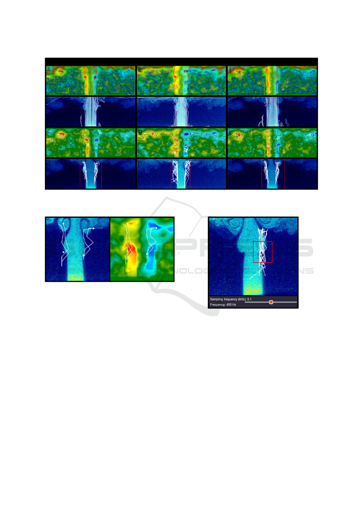
Vortex Appearance Frequency
Figure 8 displays a user-selected area defined by
points a and b, where the vortex frequency was calcu-
lated over a specified number of time steps in the sim-
ulation. Using the method described in section 4, and
with an initial sampling rate of 5.1 kHz, the vortex
appearance frequency was determined. In this region,
the vortex trajectories revealed a frequency of 400 Hz,
underscoring the periodic nature of vortex formation
within the flow. The direct consequence of this in-
formation is that, considering such configuration, if it
emits a noise, then its fundamental frequency will be
at this given frequency.
Particle Visualisation
The tool offers a feature that allows for the visualisa-
tion of the movement of multiple particles, as demon-
strated in Figure 9. Users can select particles in vari-
ous ways: manually selecting a group of particles (a),
isolating a single particle for detailed tracking (b), or
selecting a group with a predefined shape (c). This
flexibility enables users to analyse particle trajecto-
ries in different contexts.
It is particularly useful for comparing the move-
ment of particles with that of vortex cores, providing
deeper insight into how particles behave in rotation-
dominated regions versus shear-dominated regions.
By overlaying particle paths with vortex trajectories,
it helps examining the interaction between the general
flow and specific vortex structures, offering a com-
prehensive understanding of the dynamics within the
flow field.
Discussion
The proposed system combines preprocessing and
real-time components to enable a multimodal and in-
teractive visualisation of flow dynamics. By using the
Γ
2
criterion on velocity vector fields for vortex de-
tection, the tool offers the ability to explore turbulent
flow features in real time. The separation of compu-
tational tasks ensures that time-sensitive operations,
such as vortex tracking and frequency computation,
can occur interactively without compromising perfor-
mance. Moreover, the vortex tracking algorithm relies
heavily on the accuracy of the precomputed velocity
fields, and any noise in the data may lead to inaccura-
cies in the trajectory visualisation. Although the sys-
tem provides methods to smooth trajectories, future
work could focus on improving trajectory interpola-
tion techniques to further reduce the impact of noisy
data.
GRAPP 2025 - 20th International Conference on Computer Graphics Theory and Applications
228

a
b
c
d
e
f
g
h
i
j
k
l
Re = 4700 Re = 4800 Re = 5356
1110Hz
1740Hz
1050Hz
Figure 6: Multimodal visualisation of three datasets, corresponding to various Reynolds numbers, acquired with a sampling
rate of 3kHz: (a, e, i) Γ
2
and vector fields ; (b, f, j) Frame capture and particle tracking; (c, g, k) Γ
2
and level sets; (d, h, l)
Frame capture, vortex frequency calculation and resulting frequency.
a
b
Figure 7: Multimodal visualisation of a single frame. (a)
frame captures, vortex cores and trajectories; (b) Γ
2
texture,
vortex cores and trajectories.
6 CONCLUSION
This article presents a lightweight, web-based visu-
alisation system designed for tracking and analysing
vortex dynamics in airflow experiments. It pro-
vides interactive tools for visualising flow veloc-
ity, vortex identification, and tracking by utilising
high-frequency images and computed velocity vec-
tor fields. The system relies on the Γ
2
criterion to
detect vortex cores and effectively differentiate be-
tween rotation-dominated and shear-dominated flow
regions. It offers a multimodal visualisation approach
by combining captured images, vortex trajectories,
and level sets derived from Γ
2
values. This compre-
hensive view of flow dynamics enables users to ob-
serve interactions between vortices, track the evolu-
tion of flow patterns, and better understand the for-
a
b
Figure 8: Vortex appearance frequency, for a given zone ab
(red rectangle) and sampling frequency (slider). In white,
all the vortex core trajectories passing through ab.
mation of acoustic phenomena. The inclusion of fea-
tures such as vortex appearance frequency computa-
tion from selected regions further enhances the sys-
tem’s capacity to reveal intricate behaviors within the
experimental setup.
Our system has smooth performance but results in
a large memory footprint for extensive datasets. Fu-
ture improvements consist in implementing real-time
processing for specific calculations, reducing delays
while maintaining interactivity during extended visu-
alisations, or considering out-of-core techniques.
The current implementation uses Particle Image
Velocimetry (PIV) data. Since the acquisition system
is compatible with Stereo PIV setups (El Zohbi et al.,
2024), with two spatially separated camera views, 3D
Lightweight Visualisation for Vortex Tracking in Airflow Acquisition
229

a
b
c
Figure 9: Visualisation of particles selected from the user
interface: (b) single particle, (a,c) groups of particles.
visualisation becomes possible by registering datasets
into a shared space. This would provide a more im-
mersive view of flow phenomena, enhancing both vi-
sualisation and analysis.
Another interesting feature would be to compare
flow predictions coming from simulations, to pre-
dict the acoustic effects generated by an experimental
configuration. Such capabilities would enable physi-
cists to predict noise production in advance, reduc-
ing costly trial-and-error experimentation and aiding
in designing quieter, more efficient systems.
ACKNOWLEDGEMENTS
This work has been funded by the VIPER project (Ré-
gion Nouvelle Aquitaine), and MIRES federation for
research CNRS (FR3423).
REFERENCES
Ahrens, J., Geveci, B., Law, C., Hansen, C., and John-
son, C. (2005). 36-paraview: An end-user tool for
large-data visualization. The Visualization Handbook,
717:50038–1.
Assoum, H. H., Hamdi, J., El Hassan, M., Mrach, T.,
Abed Meraim, K., and Sakout, A. (2020). Energy
transfers between aerodynamic and acoustic fields in
a rectangular impinging jet. Energy Reports, 6:812–
816.
Ayachit, U., Bauer, A., Geveci, B., O’Leary, P., Moreland,
K., Fabian, N., and Mauldin, J. (2015). Paraview cat-
alyst: Enabling in situ data analysis and visualization.
In Proceedings of the First Workshop on In Situ Infras-
tructures for Enabling Extreme-Scale Analysis and Vi-
sualization, pages 25–29.
Ayachit, U., Whitlock, B., Wolf, M., Loring, B., Geveci,
B., Lonie, D., and Bethel, E. W. (2016). The sen-
sei generic in situ interface. In 2016 Second Work-
shop on In Situ Infrastructures for Enabling Extreme-
Scale Analysis and Visualization (ISAV), pages 40–44.
IEEE.
Bush, J. W. (2004). Surface tension mod-
ule. URL http://web.mit.edu/1.63/www/Lec-
notes/Surfacetension.
Childs, H., Brugger, E., Whitlock, B., Meredith, J., Ahern,
S., Pugmire, D., Biagas, K., Miller, M., Harrison, C.,
Weber, G. H., et al. (2012). Visit: An end-user tool for
visualizing and analyzing very large data.
DaVIS (2024). https://www.lavision.de/en/products/davis-
software/.
Dorier, M., Sisneros, R., Peterka, T., Antoniu, G., and
Semeraro, D. (2013). Damaris/viz: A nonintru-
sive, adaptable and user-friendly in situ visualization
framework. In 2013 IEEE Symposium on Large-Scale
Data Analysis and Visualization (LDAV), pages 67–
75. IEEE.
El Zohbi, B., Assoum, H. H., Alkheir, M., Afyouni,
N., Abed Meraim, K., Sakout, A., and El Hassan,
M. (2024). Experimental investigation of the aero-
acoustics of a rectangular jet impinging a slotted plate
for different flow regimes. Alexandria Engineering
Journal, 87:404–416.
Graftieaux, L., Michard, M., and Grosjean, N. (2001).
Combining piv, pod and vortex identification algo-
rithms for the study of unsteady turbulent swirling
flows. Measurement Science and Technology,
12(9):1422.
Gutmark, E., Wolfshtein, M., and Wygnanski, I. (1978).
The plane turbulent impinging jet. Journal of Fluid
Mechanics, 88(4):737–756.
Kuhlen, T., Pajarola, R., and Zhou, K. (2011). Parallel in
situ coupling of simulation with a fully featured vi-
sualization system. In Proceedings of the 11th Euro-
graphics Conference on Parallel Graphics and Visu-
alization (EGPGV), volume 10, pages 101–109. Eu-
rographics Association.
Sakakibara, J., Hishida, K., and Phillips, W. R. (2001). On
the vortical structure in a plane impinging jet. Journal
of Fluid Mechanics, 434:273–300.
Sarton, J., Zellmann, S., Demirci, S., Güdükbay, U.,
Alexandre-Barff, W., Lucas, L., Dischler, J.-M., Wes-
ner, S., and Wald, I. (2023). State-of-the-art in large-
scale volume visualization beyond structured data. In
Computer Graphics Forum, volume 42, pages 491–
515. Wiley Online Library.
Sommerfeld, A. (1909). Ein beitrag zur hydrodynamischen
erklärung der turbulenten flüssigkeitsbewegungen. In-
ternational Congress of Mathematicians, 3:116–124.
Yokobori, S., Kasagi, N., and Hirata, M. (1983). Trans-
port phenomena at the stagnation region of a
two-dimensional impinging jet. Trans. JSME B,
49(441):1029–1039.
GRAPP 2025 - 20th International Conference on Computer Graphics Theory and Applications
230