Generative Adversarial Network for Image Reconstruction from

Human Brain Activity

Tim Tanner

and Vassilis Cutsuridis

1,2 b

School of Computer Science, University of Lincoln, Lincoln, U.K.

School of Engineering, Computing and Mathematics, University of Plymouth, Plymouth, U.K.

Keywords: Visual Perception, EEG, AC-GAN, Thought Decoding, Image Generation, Classification, Embedding,

Modulation Layer.

Abstract: Decoding of brain activity with machine learning has enabled the reconstruction of thoughts, memories and

dreams. In this study, we designed a methodology for reconstructing visual stimuli (digits) from human brain

activity recorded during passive visual viewing. Using the MindBigData EEG dataset, we preprocessed the

signals and cleaned them from noise, muscular artifacts and eye blinks. Using the Common Average

Reference (CAR) method and past studies’ results we reduced the available electrodes from 14 to 4 keeping

only those containing discriminative features associated with the visual stimulus. A convolutional neural

network (CNN) was then trained to encode the signals and classify the images. A 92% classification

performance was achieved post-CAR. Three variations of an auxiliary conditional generative adversarial

network (AC-GAN) were evaluated for decoding the latent feature vector with its class embedding and

generating black-and-white images of digits. Our objective was to create an image similar to the presented

stimulus through the previously trained GANs. An average 65% reconstruction score was achieved by the

AC-GAN without a modulation layer, a 60% by the AC-GAN with modulation layer and multiplication, and

a 63% by the AC-GAN with modulation and concatenation. Rapid advances in generative modeling promise

further improvements in reconstruction performance.

1 INTRODUCTION

In our everyday lives we are bombarded with visual

stimuli for which we form visual memories of them

and of their between associations. A defining feature

of visual cognition is our ability to imagine these

stored memories even in the absence of any stimulus,

allowing us to escape from the limitations of our

current perspective into a limitless range of virtual

worlds (Fulford et al., 2018). But how does our brain

store and retrieve visual memories even in the

presence/absence of a visual stimulus? Which brain

areas participate in this visualization process? Can we

decode our brain signals and reconstruct these visual

representations? The scope of this study is to address

these questions. Utilizing the MindBigData dataset of

brain signals via EEG during passive visual viewing

of images of digits (0-9) from the MNIST dataset we

employed an encoder (a CNN) to extract the latent

feature vector from these brain signals and a decoder

https://orcid.org/0009-0009-5908-6869

https://orcid.org/0000-0001-9005-0260

(a GAN) to reconstruct the images viewed while these

brain signals were recorded. The quality of the

reconstructed images was then compared to the

ground truth (MNIST images) using two performance

metrics (the Dice and Structural Similarity Index

scores) and inferences were drawn.

2 RELATED WORK

The reconstruction of high-quality perceived or

imagined images from brain signals always laid in the

realm of science fiction. Recent advancements in

generative AI (GANs) have allowed scientists to turn

the image reconstruction from brain signals into a

reality. Below we provide a brief overview of some

of these attempts. Kavasidis and colleagues (2017)

employed an encoder (an LSTM layer), which aimed

to identify a latent feature space for brain signal

classification, and a decoder (a VAE or a GAN),

868

Tanner, T. and Cutsuridis, V.

Generative Adversarial Network for Image Reconstruction from Human Brain Activity.

DOI: 10.5220/0013149300003911

Paper published under CC license (CC BY-NC-ND 4.0)

In Proceedings of the 18th International Joint Conference on Biomedical Engineering Systems and Technologies (BIOSTEC 2025) - Volume 1, pages 868-877

ISBN: 978-989-758-731-3; ISSN: 2184-4305

which turned the learned feature into images using a

deconvolution approach. Their encoder reached an

86% classification accuracy, whereas their decoder

achieved a below average image reconstruction

quality. Tirupattur and colleagues (2018) employed

an 1D-CNN and modified DC-GAN to generate

images from thought using EEG signals with average

generation success. Jiao et al. (2019) the EEG data

were first converted into EEG Map image, which was

further encoded using visual CNN. The brain signal

classification accuracy was approximately 93%. The

encoded signal was then used with a GAN to

reconstruct high quality perceived images. Recently,

Khare et al. (2022) developed a pipeline consisting of

a feature extractor based on a mixture of LSTM and

gated recurrent neural network layers in order to

extract important visual features from the EEG data

regarding the type and structure of visual stimuli. The

mapping between the extracted feature vector and the

corresponding image was learned using Conditional

Progressive GAN (cProGAN). After training and

testing on a publicly available dataset, their EEG

classifier was able to achieve 98.8% test accuracy,

and cProGAN achieved an inception score (IS) of

5.15 surpassing the previous best 5.07 IS.

3 MATERIALS AND METHODS

3.1 EEG Data

The EEG used in our study was part of the

MindBigData dataset of Vivancos and Cuesta (2022).

Briefly, a human participant was seated in front of a

65’’ TV screen viewing for 2 seconds a single digit

from 0 to 9. Each digit was presented in white font

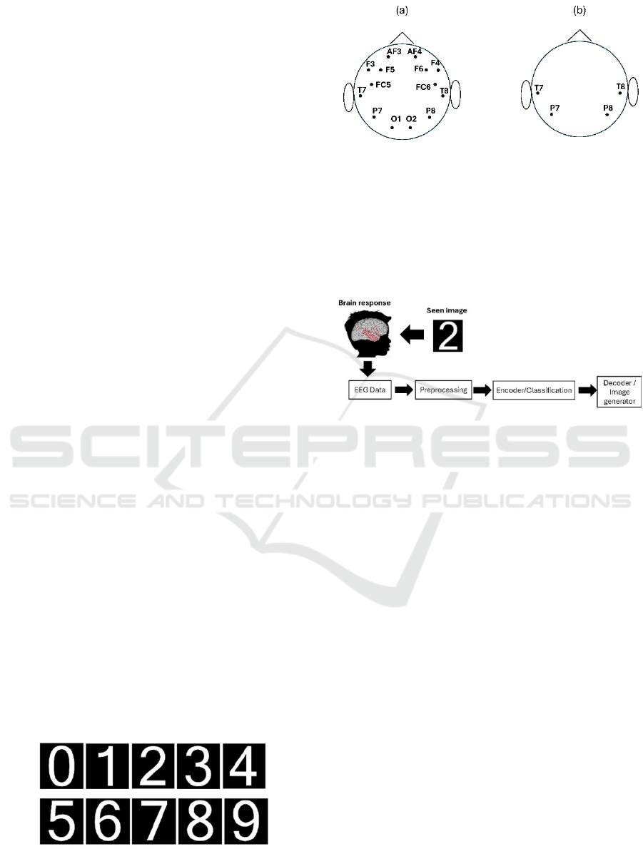
over full black background (see Fig. 1). The order of

presentation of the digits was random with a black

screen in between them. The brain activity of the

human participant was recorded using a 14-channel

(AF3, AF4, F7, F8, F3, F4, FC5, FC6, T7, T8, P7, P8,

O1 & O2) Emotiv EPOC device (see Fig. 2a) at an

average sampling rate of 128Hz resulting in ~52000

brain signals (see Table 1).

Figure 1: Idealized MNIST stimuli (digits from 0 to 9).

Figure 2: (a) Emotiv EPOC electrode positions (Stytsenko

et al., 2011). (b) Four electrode positions used in our study.

3.2 Algorithmic Pipeline

Our high-level algorithmic pipeline is depicted in Fig.

3. Every step in the pipeline is described in detail in

the subsequent sections.

Figure 3: Algorithmic pipeline (from EEG data collection

to image reconstruction).

3.2.1 Signal Preprocessing

EEG signals are noisy and full of artifacts. A zero-

phase AC notch filter at 50Hz with a 1hz band was

applied to the raw EEG data to remove any effects

from line noise potentially created by interference

from the mains 50hz circuits. Since the oscillation

signals are typically in the range of µVs, AC

fluctuations can completely overwhelm these signals.

Next, a 5th order Butterworth, non-causal bandpass

filter was applied using a 0.4hz low-pass and 60Hz

high-pass band limits to keep only those frequencies

relevant to visual perception (0.4-60Hz). A -6db

cutoff frequency was applied to both band limits and

a Hamming window with 0.0194 passband ripple was

used. Next, the functionality of the MNE package

(Gramfort et al. 2013) was utilized to remove epochs

contaminated with muscular artifacts and eye blinks.

A maximum 100µV peak-to-peak threshold was set

based on previous studies (Sanei and Chambers

2013). Epochs which exceeded this threshold level

were excluded from further analysis (see Table 1).

Generative Adversarial Network for Image Reconstruction from Human Brain Activity

869

Table 1: EEG signals per class (digit).

Class

label

Raw EEG

signals

from MBD

EEG signals

after MNE

thresholdin

EEG signals

after CARs

0 5212 3845 1180

1 5080 3798 1090

2 5196 3809 1130

3 5294 3950 1100

4 5079 3765 1100

5 5256 3916 1180

6 5218 3868 1170

7 5069 3780 1195

8 5241 3861 1115

9 5250 3917 1150

Total 51895 38509 11410

Because the Emotiv EPOC device uses no

reference signal, we employed the CAR method

(Mishra et al., 2021), which required to first calculate

the average signal from all 14 channels for each digit,

and then calculate the correlation coefficient ρ

between each channel signal and the mean signal for

each digit. The value of correlation coefficient is in

between -1 to +1. If the value of the correlation

coefficient was high, that meant the channel signal

was closer to the mean signal and thus it could be

considered as less noisy. We selected only those

signals that were having a correlation coefficient

greater than a certain threshold (ρ > 0.9) (see Table

1). Finally, the signal-to-noise ratio (SNR) was

calculated for all digit signals before CAR and after

CAR to assess the effectiveness of the CAR method

(see Table 2).

Table 2: Final selected EEG signals per class at the end of

the preprocessing pipeline. SNR measure of effectiveness

of filtering, epoch rejection and correlation.

SNR

Class

label

Before

CAR

After CAR

(ρ>0.9)

Final selected

EEG signals

0 0.378 2.126 203

1 0.521 2.213 204

2 0.374 2.131 191

3 0.352 2.239 193

4 0.323 2.191 193

5 0.312 2.068 196

6 0.474 2.139 197

7 0.299 1.983 194

8 0.382 2.155 195

9 0.280 2.077 192

Total 1958

As Mishra and colleagues (2021) have shown T7,

P7, T8 and P8 channels are the only electrodes

containing discriminative features associated with the

visual stimulus. Based on their prediction we used

only these four-channel data (see Fig. 2b) for further

processing. These data consisted of 256-time samples

and the associated class label, which were then

resampled using a sliding window of 32 samples with

a 4-sample overlap. This resulted in each channel

being split into 9 x 32 matrix x 4 channels per class

label. The result of this segmentation was to increase

the number of training examples.

The resulting data were then split into 80% for

training and 20% for testing. The 80% training data

were further split into 75% for training and 25% for

validation.

3.2.2 Encoding and Classification

For the encoding and classification of the EEG data,

a CNN (see Supplementary Table 1 for CNN design)

was used consisting of sets of 2D convolutional layers

where the kernel size was changed so that both time

and channel axis were passed through the convolution

together keeping any relation within the same set of

filters. To achieve this the first layer had its kernel

size oriented to the time axis, the second layer

changed its orientation to the channel axis after which

a max pooling layer was used to concentrate the key

activations. A further two 2D convolutional layers

were used to increase the filters with the intention of

producing a more detailed set of filters to identify the

smaller interactions. The output from the

convolutional block was then flattened before passing

onto a set of fully connected (FC) layers. Batch

normalization was used before and after the

convolutional block to help with regularization. The

FC block took the output vector from the

convolutional block and reduced the latent dimension

down to the final output dimension of 128, using a

10% dropout between each FC layer again to help

with regularization and stopped potential over

training. The final FC layer was also batch

normalised; and used as the latent space vector for

input to the GAN generator. This layer was finally

passed to the FC layer with a softmax activation and

10 nodes to determine the classification probability

distribution.

The loss function was based on categorical cross-

entropy, as the class labels were one-hot encoded

before being used. Optimization of the loss function

was achieved using adaptive moment estimation

(Adam) method with a starting rate of 0.001 and

momentum 0.8. The final two layers are outputs from

the network, predicted label, and encoded EEG latent

space vector. The network was trained for a

maximum of 150 epochs, with a batch size of 128.

BIOSIGNALS 2025 - 18th International Conference on Bio-inspired Systems and Signal Processing

870

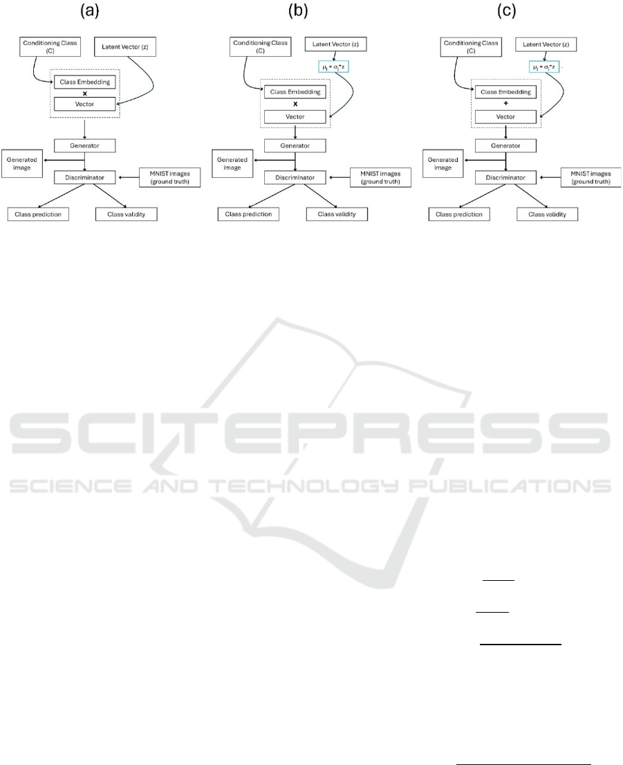
Figure 4: AC-GAN model architectures. (a) AC-GAN without a modulation layer. The conditional class embedding is

multiplied with latent vector (z). (b) AC-GAN with a modulation layer. The conditional class embedding is multiplied with

the modulated vector (µ

+ σ

• z). (c) AC-GAN with a modulation layer. The conditional class embedding is concatenated

with the modulated vector (µ

+ σ

• z).

3.2.3 Decoding and Reconstruction

For decoding and image generation, a AC-GAN

(Odena et al. 2017) was used. In the original AC-

GAN, every generated sample has a corresponding

conditioning class label, c in addition to the noise z.

In our study the noise z is replaced by the latent vector

Latent(z) of the encoder. The generator (see

Supplementary Table 2) then uses both the Latent(z)

and the Conditioning label c to generate images X

fake

= G(c; Latent(z)). The discriminator (see

Supplementary Table 3) gives both a probability

distribution over sources and a probability

distribution over the class labels, P(S j X); P(C j X) =

D(X). The objective function has two parts: the log-

likelihood of the correct source, L

, and the log-

likelihood of the correct class, L

𝐿



= 𝐸[𝑙𝑜𝑔 𝑃(𝑆 = 𝑟𝑒𝑎𝑙 | 𝑋



)] + 𝐸[𝑙𝑜𝑔 𝑃(𝑆 =

𝑓𝑎𝑘𝑒 | 𝑋



)] (1)

𝐿



= 𝐸[𝑙𝑜𝑔 𝑃(𝐶 = 𝑐 | 𝑋



)] + 𝐸[𝑙𝑜𝑔 𝑃(𝐶 =

𝑐 | 𝑋



)] (2)

D is trained to maximize L

+ L

while G is trained

to maximize L

- L

In some simulations, we added an extra layer

(modulation layer) before the generator, which

allowed the modulation of the latent feature space as

a weighted deterministic function of µ

and σ

described in (Gurumurthy et al., 2017):

𝜇



+𝜎



∗𝑧 (3)

Our objective was then to learn µ

, σ

, and the AC-

GAN parameters in order to maximize p

data

G((µ

+σ

*Latent(z))|Latent(z)). During the training

of the AC-GAN on the EEG data, we explored three

different architectures of it (see Fig. 4): (a) No

modulation layer, (b) Multiplication of the

modulation layer with the conditional class

embedding, and (c) Concatenation of the modulation

layer with the conditional class embedding. The

training was left to run for 2000 epochs after which

time image generation was stabilized. An Adam

optimizer with learning rate of 0.0002, beta = 0.5 and

decay of 1e-6 was used for both the generator and

discriminator.

3.2.4 Performance Metrics

We used the following metrics for evaluating the

performances of our classifier:

𝑃𝑟𝑒𝑐𝑖𝑠𝑖𝑜𝑛 =





(4)

𝑅𝑒𝑐𝑎𝑙𝑙 =





(5)

𝐹1 𝑠𝑐𝑜𝑟𝑒 = 2 ∗

∗



(6)

where TP are the true positives, TN are the true

negatives, FP are the false positives and FN are the

false negatives.

We used the following metrics for evaluating the

performance of our image generator:

𝐷𝑖𝑐𝑒 𝑠𝑐𝑜𝑟𝑒 = 2 ∗

|∩ |

||| |

(7)

This metric evaluates the similarity between two

images, the predicted one (generated) against the

ground truth (MNIST image). Its value ranges

between 0 and 1, with 1 being the perfect overlap

Generative Adversarial Network for Image Reconstruction from Human Brain Activity

871

(100% similarity between the predicted and the

ground truth) and 0 being no overlap (0% similarity).

The Structural Similarity Index Measure (SSIM)

is a perceptual metric used to evaluate the quality of

generated images by comparing them directly to

ground truth images. Unlike traditional measures like

Mean Squared Error (MSE) that only assess pixel-by-

pixel differences, SSIM considers human visual

perception, focusing on structural information,

luminance, and contrast to assess image similarity. It

produces a score between -1 and 1, where 1 indicates

perfect similarity. SSIM is calculated by comparing

local patterns of pixel intensities normalized for

luminance and contrast, providing a more holistic

view of image quality. It is particularly useful for

evaluating image generation tasks, such as super-

resolution, denoising, and inpainting, where

maintaining structural fidelity and visual quality is

crucial. By accounting for variations in structure,

texture, and lighting, SSIM offers a robust measure of

how closely generated images resemble their

corresponding ground truth, making it an effective

tool for evaluating generative models:

𝑆𝑆𝐼𝑀

(

𝑥, 𝑦

)

=(𝑙

(

𝑥, 𝑦

)



∗(𝑐

(

𝑥, 𝑦

)



∗(𝑠(𝑥,𝑦))



(8)

where

𝑙(𝑥, 𝑦) = (2𝜇𝑥 ∗ 𝜇𝑦 + 𝐶1)/(𝜇𝑥



+ 𝜇𝑦



+𝐶1)

𝑐(𝑥, 𝑦) = (2𝜎𝑥 ∗ 𝜎𝑦 + 𝐶2)/(𝜎𝑥



+ 𝜎𝑦



+𝐶2)

𝑠(𝑥, 𝑦) = (𝜎𝑥𝑦 + 𝐶3)/(𝜎𝑥 ∗ 𝜎𝑦 + 𝐶3)

where µ is the mean pixel value, σ is the standard

deviation of the pixel value and σxy is the covariance

of the pixel value. C1, C2, and C3 are constraints to

avoid division by zero with C3 = C2 /2. α, β, and γ are

positive exponents that change the components

contribution to the overall SSIM.

4 RESULTS

4.1 Classification

Our CNN model was trained on two sets of data. The

post filtered data prior to CAR correlation selection

method and the data set after final CAR correlation

selection. From Tables 6 and 7, it is evident that

accuracy improves from an approximate average 46%

in the pre-CAR selection case to an approximate

average 92% in the post-CAR selection case.

Table 3: CNN evaluation after trained with pre-CAR

selection data.

Label precision Recall F1-score

0 0.48 0.48 0.48

1 0.46 0.43 0.45

2 0.43 0.40 0.41

3 0.50 0.51 0.51

4 0.46 0.39 0.42

5 0.45 0.48 0.46

6 0.45 0.46 0.45

7 0.41 0.47 0.47

8 0.43 0.43 0.43

9 0.50 0.47 0.47

Accurac

0.46

Micro avg 0.46 0.46 0.46

Wei

hted av

0.46 0.46 0.46

Table 4: CNN evaluation after trained with post-CAR

selection data.

Label precision Recall F1-score

0 0.92 0.88 0.90

1 0.93 0.90 0.92

2 0.91 0.87 0.89

3 0.94 0.94 0.94

4 0.91 0.93 0.92

5 0.89 0.91 0.90

6 0.92 0.89 0.90

7 0.90 0.96 0.93

8 0.93 0.95 0.94

9 0.92 0.93 0.93

Accurac

0.92

Micro av

0.92 0.92 0.92

Wei

hted av

0.92 0.92 0.92

Figures 5 and 6 show the confusion matrix

between class predictions, and the t-SNE map of class

separability, respectively, before the application of

the CAR selection method. Both figures clearly show

the extent of class confusion which is caused by the

remaining noise in the signals prior to extracting the

data which had a high correlation threshold.

In contrast, figures 7 and 8 show the confusion

matrix between class predictions, and the t-SNE map

of class separability, respectively, after the

application of the CAR selection method. It is clearly

evident that the classes are mostly separable and very

little confusion between them is present.

4.2 Image Reconstruction

From Figure 9 it is clear that the AC-GAN with no

modulation layer is able to reconstruct well all digits

with the exception of ‘2’, which confuses it with ‘0’.

The SSIM score for ‘2’ is 0.098 (see Table 5).

BIOSIGNALS 2025 - 18th International Conference on Bio-inspired Systems and Signal Processing

872

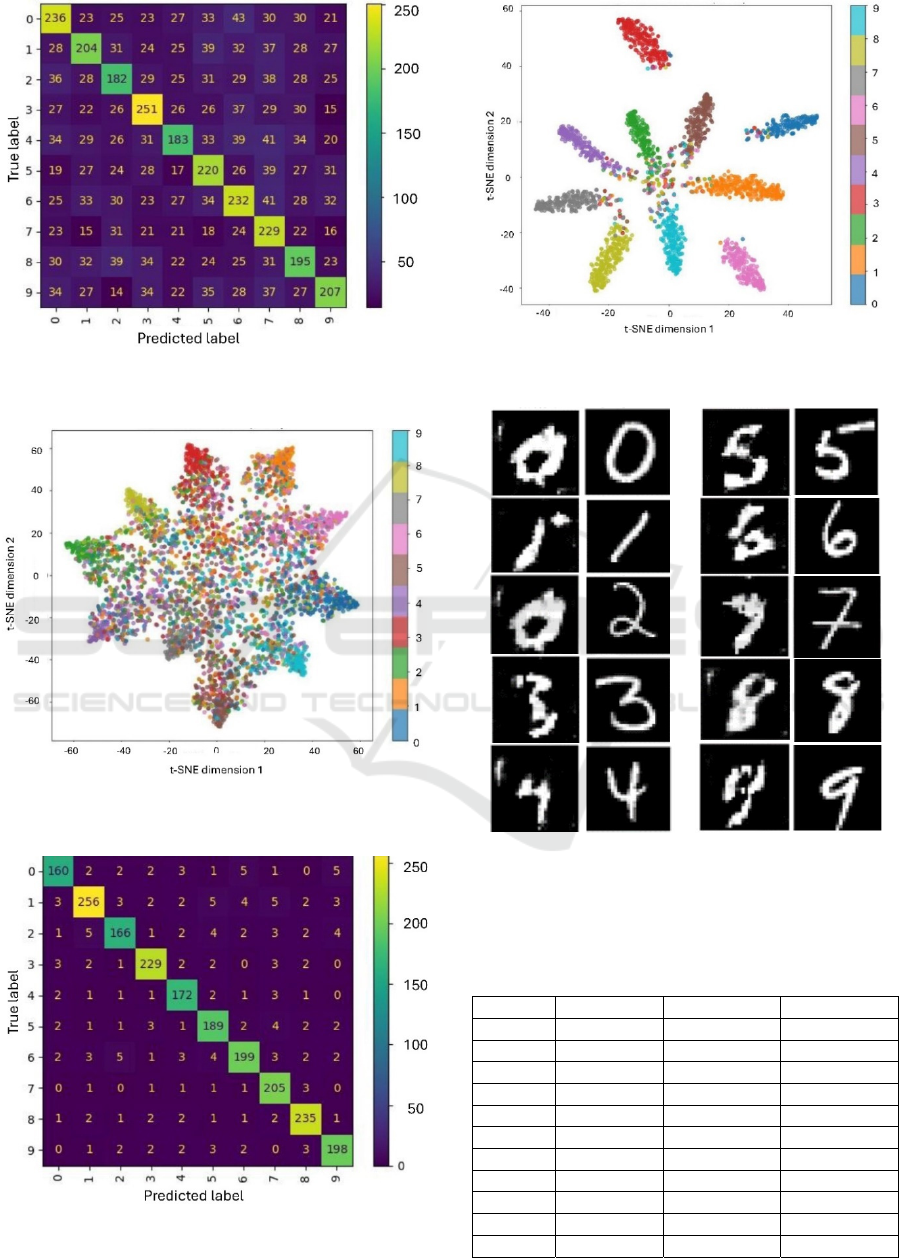
Figure 5: Class confusion matrix of CNN model trained

with pre-CAR selection data.

Figure 6: t-SNE class separability of CNN model trained

with pre-CAR selection data.

Figure 7: Class confusion matrix of CNN model trained

with post-CAR selection data.

Figure 8: t-SNE class separability of CNN model trained

with post-CAR selection data.

Figure 9: Reconstruction of digit (0-9) images (columns 1

and 3) compared to the MNIST digit (0-9) images (columns

2 and 4) by the AC-GAN without a modulation layer (see

Fig. 4a for GAN architecture)

Table 5: Summary of reconstruction evaluation results of

AC-GAN without a modulation layer.

Label Prediction Dice score SSIM score

0 TRUE 0.581 0.229

1 TRUE 0.408 0.449

2 FALSE 0.285 0.098

3 TRUE 0.437 0.293

4 TRUE 0.408 0.380

5 TRUE 0.467 0.316

6 TRUE 0.567 0.401

7 TRUE 0.198 0.139

8 TRUE 0.568 0.271

9 TRUE 0.454 0.334

Average 0.4373 0.291

Generative Adversarial Network for Image Reconstruction from Human Brain Activity

873

From Figure 10 it is clear that the AC-GAN with

modulation layer and multiplication of the modulated

latent vector with the conditioning class embedding is

able to reconstruct well all digits with the exception

of ‘6’, which confuses it with ‘5’. The SSIM score for

‘6’ is 0.118 (see Table 6). Similarly, the SSIM score

for ‘5’ is 0.115 even though the model is able to

reconstruct the correct digit.

Figure 10: Reconstruction of digit (0-9) images (columns 1

and 3) compared to the MNIST digit (0-9) images (columns

2 and 4) by the AC-GAN with a modulation layer and

multiplication of the modulated latent vector with the

conditional class embedding (see Fig. 4b for GAN

architecture).

Table 6: Summary of reconstruction evaluation results of

AC-GAN with a modulation layer (multiplication of the

modulated latent vector with the conditional class

embedding).

Label Prediction Dice score SSIM score

0 TRUE 0.538 0.128

1 TRUE 0.467 0.474

2 TRUE 0.476 0.184

3 TRUE 0.446 0.218

4 TRUE 0.416 0.193

5 TRUE 0.370 0.115

6 FALSE 0.234 0.118

7 TRUE 0.159 0.164

8 TRUE 0.415 0.281

9 TRUE 0.382 0.199

Average 0.39 0.2074

From Figure 11 it is clear that the AC-GAN with

modulation layer and concatenation of the modulated

latent vector with the conditioning class embedding is

able to reconstruct well all digits with the exception

of ‘0’, which confuses it with ‘2’. The SSIM score for

‘0’ is 0.064 (see Table 7).

Figure 11: Reconstruction of digit (0-9) images (columns 1

and 3) compared to the MNIST digit (0-9) images (columns

2 and 4) by the AC-GAN with a modulation layer and

concatenation of the modulated latent vector with the

conditional class embedding (see Fig. 4c for GAN

architecture).

Table 7: Summary of reconstruction evaluation results of

AC-GAN with a modulation layer (concatenation of the

modulated latent vector with the conditional class

embedding).

Label Prediction Dice score SSIM score

0 FALSE 0.155 0.064

1 TRUE 0.130 0.151

2 TRUE 0.321 0.205

3 TRUE 0.473 0.323

4 TRUE 0.446 0.393

5 TRUE 0.466 0.225

6 TRUE 0.421 0.195

7 TRUE 0.379 0.291

8 TRUE 0.482 0.409

9 TRUE 0.296 0.255

Average 0.3569 0.2511

5 DISCUSSION

Our study has produced interesting results regarding

the reconstruction of mental content (visual stimulus)

from EEG with generative AI by leveraging the latent

vector (not random noise) and a predicted semantic

(class) embedding. The study demonstrated that EEG

BIOSIGNALS 2025 - 18th International Conference on Bio-inspired Systems and Signal Processing

874

signals can effectively be processed to extract

meaningful features, which, when fed into a trained

classification encoder and a subsequent generative

network, can generate representative images of the

perceived visual stimulus. When comparing the SSIM

scores of the AC-GAN models, we found that the

model with the best reconstruction score was the AC-

GAN without modulation (Average SSIM = 0.291 or

65% average similarity between the generated images

and the ground truth). The model with the worst

reconstruction score was the AC-GAN with

modulation and multiplication (Average SSIM =

0.2074 or 60% average similarity between the

generated images and the ground truth). The average

Dice scores for the three AC-GAN models were

lower than the average SSIM scores (Average Dice

for AC-GAN without modulation = 43.73%; Average

Dice for AC-GAN with modulation and

multiplication =39%; Average Dice for AC-GAN

with modulation and concatenation = 35.69%). Since

the Dice score depends solely on the similarity

between the reconstructed images and the ground

truth on a pixel-by-pixel basis and excludes any

structural information, luminance, and contrast

information from the evaluation, then the SSIM score

is a more accurate reconstruction metric.

In this study, we utilized EEG data collected from

a different group (MindBigData (Vivancos and

Cuesta, 2022)) to which we had no control of their

experimental design, recording and collection

processes. Furthermore, EEG signals by nature are

noisy, full of muscular artifacts and eye blinks

particularly the signals from the frontal electrodes.

Careful preprocessing of the MindBigData EEG

signals reduced the data for training and testing from

51895 samples to 1958 samples, which was only

3.77% of the total data set. Even though the final EEG

dataset used for encoding and classification was

small, our CNN model reached a 92% classification

performance on average, which is close to the current

state-of-the-art (~96% (Mahapatra and Bhuyan,

2023)). Given the single-subject nature of these data,

it is unclear how the results would generalize to a

larger population. We believe this could be a fruitful

area for future investigation.

Despite the AC-GAN model's ability to generate

conditioned images, it is unable to rectify

misclassifications based solely on the encoded EEG

latent vector and conditioning label. As a result, when

the model generates an image that is incorrectly

classified, the resulting image exhibits a low SSIM

score, indicating poor similarity to the ground truth

(e.g. reconstructed ‘2’ digit by the AC-GAN without

modulation (see Fig. 9), or reconstructed ‘0’ digit by

the AC-GAN with modulation and concatenation (see

Fig. 11)). Paradoxically in some cases, this

misclassified image may still receive a relatively high

score, suggesting a potential discrepancy between the

model's perception of the image and its actual fidelity

to the ground truth (e.g. reconstructed ‘6; digit by the

AC-GAN with modulation and multiplication (see

Fig. 10)). This is because in the current model design

the predicted class conditioning label has a higher

influence on the predicted image over the encoded

latent vector.

A future extension to our study would be to

include a reinforcement learning agent applied to the

class label prediction. This agent would penalize the

incorrect class label thus reducing its influence on the

predicted image over the encoded latent vector.

Which in cases where the classification is incorrect

the agent would provide unsupervised learning

adjustments which may help to correct the AC-GAN

prediction and validity to indicate an uncertain score.

ACKNOWLEDGEMENTS

This work was supported by the EU HORIZON 2020

Project ULTRACEPT under Grant 778062.

REFERENCES

Fulford J, Milton F, Salas D, Smith A, Simler A, Winlove

C, Zeman A. (2018). The neural correlates of visual

imagery vividness = An fMRI study and literature

review. Cortex. 105: 26-40

Goodfellow I, Pouget-Abadie J, Mirza M, Xu B, Warde-

Farley D, Ozair S, Courville A, Bengio Y. (2014)

Generative Adversarial Nets. https://arxiv.org/abs/14

06.2661

Gramfort A, Luessi M, Larson E, Engemann D, Strohmeier

D, Brodbeck C, Goj R, Jas M, Brooks T, Parkkonen L,

Hämäläinen M. (2013) MEG and EEG data analysis

with MNE-Python. Frontiers in Neuroscience.

7(267):1-13

Gurumurthy S, Sarvadevabhatla R, Babu R. (2017)

DeLiGAN: Generative Adversarial Networks for

Diverse and Limited Data. IEEE Conference on

Computer Vision and Pattern Recognition (CVPR).

IEEE. 166-174. https://doi.org/10.1109/cvpr.2017.525

Jiao Z, You H, Yang F, Li X, Zhang H, Shen D. (2019)

Decoding EEG by visual-guided deep neural networks.

IJCAI, pp. 1387–1393

Khare S, Choubey RN, Amar L, Udutalapalli V. (2022).

NeuroVision: perceived image regeneration using

cProGAN. Neural Computing and Applications 34:

5979–5991

Generative Adversarial Network for Image Reconstruction from Human Brain Activity

875

Kavasidis I, Palazzo S, Spampinato C, Giordano D, Shah

M. (2017) Brain2image: Converting brain signals into

images. Proceedings of the 25th ACM international

conference on multimedia, 1809–1817

Mahapatra NC, Bhuyan P. (2023). EEG-based

classification of imagined digits using a recurrent

neural network. J Neural Eng. 20(2)

Mishra R, Sharma K, Bhavsar A. (2021) Visual Brain

Decoding for Short Duration EEG Signals. 29th

European Signal Processing Conference (EUSIPCO).

IEEE. 1226-1230. https://doi.org/10.23919/eusipco54

536.2021.9616192.

Mishra R, Sharma K, Jha RR, Bhavsar A. (2023).

NeuroGAN: image reconstruction from EEG signals

via an attention-based GAN. Neural Computing and

Applications. 35(12): 9181-9192. https://doi.org/10.10

07/s00521-022-08178-1

Odena A, Olah C, Shlens J. (2017) Conditional Image

Synthesis with Auxiliary Classifier GANs. Proceedings

of the 34th International Conference on Machine

Learning. 70: 2642-2651

Sanei S, Chambers JA. (2013). EEG signal processing.

John Wiley & Sons

Stytsenko K, Jablonskis E, Prahm C. (2011). Evaluation of

consumer EEG device emotiv epoc. In MEi: CogSci

Conference 2011, Ljubljana, 2011.

Tirupattur P, Rawat YS, Spampinato C, Shah M. (2018)

Thoughtviz: visualizing human thoughts using

generative adversarial network. Proceedings of the 26th

ACM international conference on multimedia, 950–958

Vivancos D, Cuesta F. (2022). MindBigData 2022: A dataset

of brain signals. https://arxiv.org/pdf/2212.14746

APPENDIX

Supplementary Table 1: EEG encoder/classifier CNN

design.

Layer Output

Shape

Attributes Parameters

Input (None, 9, 32, 1)

BatchNormalization (None, 9, 32, 1) 4

2D Convolution (None, 9, 32,

128)

128 filters,

(9,1), pad 1,

same

640

2D Convolution (None, 9, 32,

64)

64 filters,

(9,1), pad 1,

same

73792

MaxPooling2D (None, 9, 16,

64)

(1, 2) 0

2D Convolution (None, 64, 13,

40)

64 filters, (4,

25), pad 1,

valid

57644

MaxPooling2D (None, 64, 6,

40)

(1, 2) 0

2D Convolution

(None, 15, 5,

128)

128 filters,

(50, 2), pad

1, valid

512128

Flatten (None, 9600) 0

BatchNormalization (None, 9600) 38400

Dense (None, 512) 512 nodes,

Relu

4915712

Dropout (None, 512) 0.1 0

Dense (None, 256) 256 nodes,

Relu

131328

Dropout (None, 256) 0.1 0

Dense (None, 128) 128 nodes,

Relu

32896

Dropout (None, 128) 0.1 0

BatchNormalization (None, 128) 512

Dense (None, 10) Softmas, L2

regularizatio

1290

Supplementary Table 2: AC-GAN generator network

model design.

Layer

Output

Shape

Attributes Parameters

Input (class

label)

(None, 1)

Embedding (None, 1, 128)

1280

Flatten (None, 128)

nput (EEG latent

space)

(None, 128)

Modulation of

EEG Layer

(None, 128)

256

Multiply (None, 128)

Dense (None, 6272)

Nodes 6272,

Relu

809088

Reshape

(None, 7, 7,

128)

Batch

Normalization

(None, 7, 7,

128)

512

UpSample2D

(None, 14, 14,

128)

nearest 0

2D Convolution

(None, 14, 14,

128)

128, kernel 3,

stride 1, pad

same, Relu

147584

Batch

Normalization

(None, 14, 14,

128)

512

UpSample2D

(None, 28, 28,

128)

Nearest 0

2D Convolution

(None, 28, 28,

64)

64, kernel 3

stride 1, pad

same, TanH

73792

Batch

Normalization

(None, 28, 28,

64)

256

2D Convolution

(None, 28, 28,

1, kernel 3,

stride 1, pad

same, Tanh

577

BIOSIGNALS 2025 - 18th International Conference on Bio-inspired Systems and Signal Processing

876

Supplementary Table 3: AC-GAN discriminator network

model design.

Layer Output Shape Attributes Parameters

Input (generated

image)

(None, 28, 28, 1)

2D Convolution

(None, 14, 14,

16)

16, kernel 3,

stride 2, pad

same

160

LeakyRelu

activation

(None, 14, 14,

16)

0.2 0

Dropout

(None, 14, 14,

16)

0.25 0

2D Convolution (None, 7, 7, 32)

32, kernel 3,

stride 2, pad

same

4640

ZeroPad (None, 8, 8, 64)

LeakyRelu

activation

(None, 8, 8, 64) 0.2 0

Dropout (None, 8, 8, 64) 0.25 0

Batch

Normalization

(None, 8, 8, 64) 0.8 128

2D Convolution (None, 4, 4, 128)

64, kernel 3,

stride 2, pad

same

18496

LeakyRelu

activation

(None, 4, 4, 128) 0.2 0

Dropout (None, 4, 4, 128) 0.25 0

Batch

Normalization

(None, 4, 4, 64) 0.8 256

2D Convolution (None, 4, 4, 128)

128, kernel 3,

stride 1, pad

same

73856

LeakyRelu

activation

(None, 4, 4, 128) 0.2 0

Dropout (None, 4, 4, 128) 0.25 0

Flatten (None, 2048 0

Dense (validity

confidence)

(None, 1) 2049

Dense (class

prediction)

(None, 10) 20490

Generative Adversarial Network for Image Reconstruction from Human Brain Activity

877