Efficient Modeling of 3D Epithelial Cell Structure Dynamics
via Backbone Spreads
Javier Buceta
1
, Stefan Funke
2
and Sabine Storandt
3 a
1
Institute for Integrative Systems Biology (I2SysBio), UV-CSIC, Valencia, Spain
2
FMI, University of Stuttgart, Germany
3
University of Konstanz, Germany
Keywords:
3D Voronoi Diagram, Cellular Geometry, Tubular Geometry, Energy Minimization, Scutoids.
Abstract:
An important means to study the morphogenesis of epithelial cell structures is faithful modeling and simu-
lation of the underlying cell dynamics. In particular, changes in cell shapes and cell neighborhoods have to
be captured to gain understanding of organ development and other complex processes. A typical 2D tissue
model is cell-center based Voronoi tessellation. However, since epithelial cells form curved layers in three-
dimensional space, a 2D model cannot encompass all relevant aspects. In this paper, we provide a formal 3D
model for epithelial cell structures based on the notion of backbone spreads and study its geometric properties.
Based thereupon, we devise a modified version of the well-known Metropolis-Hastings algorithm to find cell
tissue configurations that minimize a given energy function. We prove that our new algorithm is very efficient
from a theoretical perspective and also demonstrate its good performance in practice on the example of tubular
epithelia. Furthermore, we show that a rich set of cell shapes and connectivity structures emerge in our model,
and we analyze their frequency of occurrence with respect to the model parameters.
1 INTRODUCTION
The organization and structure of cells impact the
development and functionality of many types of tis-
sues and organs in multicellular organisms. Although
bioimaging techniques provide crucial insight into
cell arrangements and dynamics, continuous monitor-
ing of cell reconfiguration processes is intricate and
often impossible. Thus, deducing suitable cell mod-
els from existing biological and biophysical data is
tremendously helpful in simulating these processes
and evaluating the impact of the relevant parameters.
Simple epithelial tissue usually consists of a single
layer of cells in which each cell is connected to a basal
and an apical surface. Epithelia are often involved in
absorption and filtration processes and have protective
functions. As epithelium tissues do not contain blood
vessels, substances are transported via diffusion and
junctions between cells within the layer. This makes
the study of the shapes and neighborhood structures
of these cells particularly important. It is tempting to
model monolayer cell structures in 2D as this allows
for simple and robust simulation of cell dynamics. Al-
a
https://orcid.org/0000-0001-5411-3834
though such models can certainly provide valuable in-
sights (see, for example (Lau et al., 2021)), they might
not capture all relevant aspects. In their seminal work,
(G
´
omez-G
´
alvez et al., 2018) show that in curved ep-
ithelia a cell shape called scutoid (a mixture between
a frustum and a prismatoid) can occur, which has dif-
ferent neighbors on the basal and apical surfaces. An
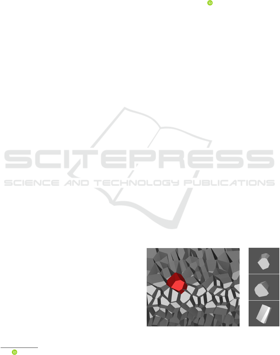
example is shown in Figure 1. Here we show the cells
with a transparent basal surface.
Figure 1: Left: Closeup of a curved epithelium. Right:
Neighborhood structure of the red cell: The basal surface
(top) has eight neighbors and the apical surface (center) has
10 due to scutoid cell shape (visible in the bottom image).
Buceta, J., Funke, S. and Storandt, S.
Efficient Modeling of 3D Epithelial Cell Structure Dynamics via Backbone Spreads.
DOI: 10.5220/0013151000003912
Paper published under CC license (CC BY-NC-ND 4.0)
In Proceedings of the 20th International Joint Conference on Computer Vision, Imaging and Computer Graphics Theory and Applications (VISIGRAPP 2025) - Volume 1: GRAPP, HUCAPP
and IVAPP, pages 89-100
ISBN: 978-989-758-728-3; ISSN: 2184-4321
Proceedings Copyright © 2025 by SCITEPRESS – Science and Technology Publications, Lda.
89

This cell shape stabilizes the tissue and thus helps
to minimize tissue energy. Such shapes only emerge
when considering cell arrangements in 3D. This and
similar findings have created the need for 3D cell
models and efficient simulation methods that can
work with them.
Two common models for cells are the vertex
model and the cell-center model. In vertex model,
cells are explicitly described by the coordinates of
their boundary vertices. In 2D, each cell coincides
with a polygon (Alt et al., 2017) and in 3D each cell is
modeled as a polyhedron (Okuda et al., 2013; Honda
et al., 2004). While the vertex model is able to cap-
ture arbitrary cell shapes, the large degree of freedom
also results in quite complicated algorithms for cell
reconfiguration and resource demanding simulations.
In the cell-center model, the cell centers are suf-
ficient to describe the entire cell arrangement since it
is assumed that the cell shapes can be derived from a
suitable tessellation. Due to their strong resemblance
to real cell structures, Voronoi tessellations are often
used for this purpose. A Voronoi tessellation for a
given point set divides the space into cells where for
each point its corresponding cell contains the portion
of the space that is closer to it than to all other input
points. This type of tessellation – also called Voronoi
diagram – works in both 2D and 3D (and beyond).
However, in 3D, a Voronoi diagram of a given point
set might not coincide with a monolayer cell structure
as it is required for epithelia, even if the diagram is re-
stricted to the space enclosed by the apical and basal
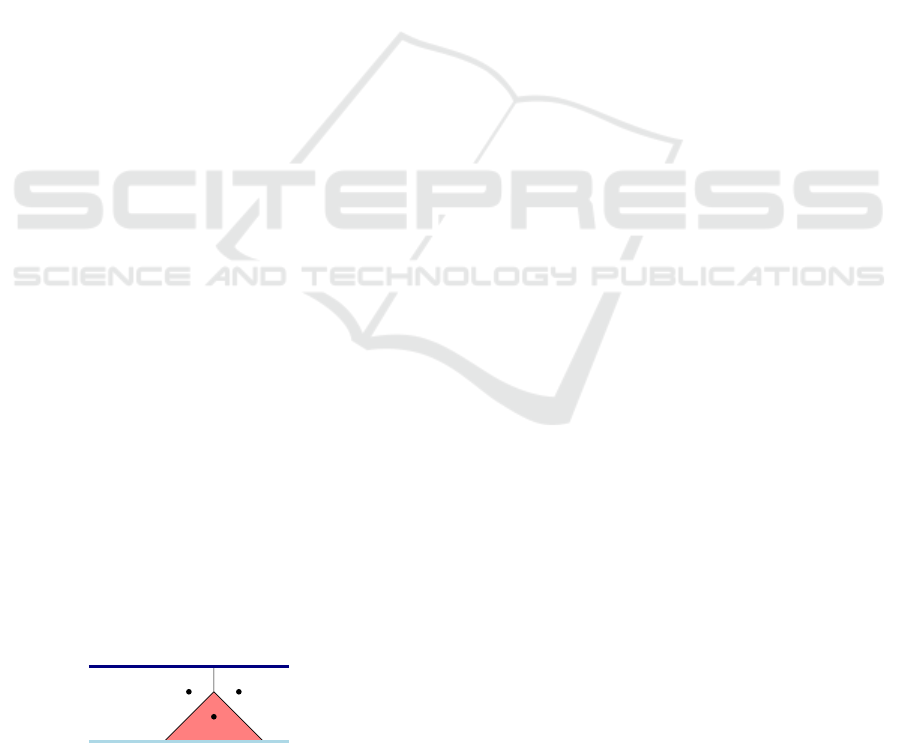
surface. Figure 2 illustrates the issue.
For the special case of tubular epithelia, a rem-
edy was proposed in (G
´
omez-G
´
alvez et al., 2022).
Here, cell centers are assumed to be known on the
apical surface and are projected to the basal surface.
The segment between the apical and the basal sur-
face intersection point is called the backbone of the
cell. A 3D Voronoi diagram for these line segments
is guaranteed to provide the desired monolayer struc-
ture. However, as the computation of Voronoi dia-
grams for line segments is very involved even in 2D,
see, e.g., (Burnikel et al., 1994a), their approach re-
lies on subsampling of the backbones and projection
of each sample to 2D. Voronoi diagrams are computed
for each 2D layer individually and then combined and
basal
apical
Figure 2: Cross section through a 3D point based Voronoi
diagram confined between the basal and apical layer. The
red cell does not reach the basal surface and thus the cell
structure does not coincide with a simple epithelium.
interpolated to estimate the 3D shapes of the cells at
each point in time during a simulation. The model
and the implementation were shown to be powerful in
describing and understanding the emergence and role
of scutoids among other cell structure phenomena.
In this paper, we provide a general parameterized
model for monolayer cell arrangements in 3D. The
model extends upon the idea of cell backbones as used
in (G
´
omez-G
´
alvez et al., 2022) but restricts their rela-
tive positions in a biological meaningful way. This al-
lows us to study geometric properties of epithelia even
before running any simulations, which is not possible
in other existing models. Furthermore, it provides us
with a framework in which we can study the complex-
ity of cell reconfiguration algorithms.
1.1 Related Work
An alternative cell-center model for epithelia based on
a given point sets was recently proposed in (Mimura
and Inoue, 2023). Here, the points are first consid-
ered in 2D and cell shapes are deduced based on a
proper triangulation of the point set. The 3D shape of
the cell is extrapolated from its 2D contour. Deforma-
tions of the basal or apical surface are used to simulate
reshaping of the tissue, as e.g. invagination. While
this impacts the 3D structure of the cells, complex cell
shapes as scutoids cannot emerge in this model.
Most other existing models rely on Voronoi di-
agrams. Voronoi diagrams have been well studied
from a computational geometry perspective. This in-
cludes dynamic Voronoi diagrams, where seed points
can move over time (Roos, 1993), 3D Voronoi dia-
grams (Ledoux, 2007), and Voronoi diagrams induced
by geometric objects as lines, line segments, balls
or polygons (Man
´
ak and Kolingerov
´
a, 2010; Held,
2001; Burnikel et al., 1994b; Alt and Schwarzkopf,
1995; Mayya and Rajan, 1996). We will discuss more
details about the relevant aspects of these data struc-
tures when we describe their role in our algorithms.
We remark, that there are also many related appli-
cations which rely on efficient dynamic Voronoi cell
reconfiguration, for example, environmental simula-
tions (Ledoux, 2008).
1.2 Contribution
We propose a novel cell-center model for 3D mono-
layer epithelia which we call tight backbone spread.
Our model allows to upper bound the number of
neighbors a cell can have a priori, based on the model
parameter. This is relevant for understanding and as-
sessing the connectivity structures of epithelia and is
also an important factor in the running time of simu-
GRAPP 2025 - 20th International Conference on Computer Graphics Theory and Applications
90

lations that study cell dynamics. In fact, we propose a
new simulation algorithm for energy minimization in
epithelia that is provably efficient on tissues adhering
to our model.
We also provide an extensive experimental evalu-
ation which demonstrates the usefulness of the model
and the algorithm in practice. Importantly, our imple-
mentation does not rely on projection to 2D Voronoi
diagrams, as done in previous work, but directly op-
erates on 3D Voronoi cells. This results in a more
faithful representation of cell shapes and neighbor-
hood structures. Indeed, we show that complex scu-
toid structures emerge in our simulations as well as
novel connectivity structures that were not described
in previous work.
2 BACKBONE SPREAD MODEL
In this section, we propose our 3D epithelium model.
A model should be general enough to capture the di-
versity of cell structures found in epithelia, but also
precise enough to gain meaningful insights from the
simulations that use the model.
Our model falls in the well-established category of
cell-center based Voronoi tessellation. However, we
use cell backbones presented as line segments instead
of single points and ensure that we always produce a
monolayer cell arrangement.
2.1 Tight Backbone Spreads
Our model needs to encompass two important as-
pects: The monolayer structure of simple epithelia
and the sensible arrangement of cells within. The
goal is to formalize these aspects solely based on the
cell backbones to align with the concept of cell-center
based models. We first focus on the second aspect, the
cell arrangement. In a real epithelium, cells should
have a certain minimum size and the sizes should not
differ too severely among different cells. Regarding
the cell backbones, this implies that they should have
a minimum distance but also that there should be a
close-by backbone to each point in the tissue. This
leads us to the following definition.
Definition 1 (Tight φ-Backbone Spread). Given a
subdomain D ⊆ R
3
and a set of line segments (back-
bones) L ⊂ D , we call (D,L ) a Tight φ-Backbone
Spread (TφBS) for φ ≥ 1 if the following two proper-
ties are met with d(.,.) denoting the Euclidean dis-
tance within D:
1. ∀L,L
′
∈ L , L ̸= L
′
: d(L,L
′
) ≥ 1
2. ∀x ∈ D : ∃L ∈ L : d(x,L) ≤ φ
The parameter φ allows to modulate the diversity
of cell sizes. So far, this model does not guarantee
a monolayer cell structure. Nevertheless, we can al-
ready explore how φ impacts the neighborhood struc-
ture of the Voronoi tessellation induced by a TφBS.
Lemma 1. Let (D , L) be a TφBS. In the 3D Voronoi
diagram V of L restricted to D, a Voronoi cell
V (L) induced by L ∈ L has O(φ
3
+ φ
2
l) neighbor-
ing Voronoi cells with l = |L| denoting the length of
segment L.
Proof. Let L
′
∈ L be a backbone such that the
Voronoi cells V (L) and V (L
′
) are neighbors. It fol-
lows that d(L,L
′
) ≤ 2φ. This holds as each point x at
the boundary of V (L) and V (L
′
) has no closer back-
bones than L and L
′
by definition of the Voronoi di-
agram, and by Property 2 of Definition 1, we know
that the distance of any point x to its closest back-
bone is not allowed to exceed φ. Therefore, every
L
′
that induces a neighboring cell to V (L) needs to
intersect the 2φ-tube around L. Furthermore, based
on Property 1 of Definition 1, we know that the 1-
tube around L
′
has to be void of any other back-
bone points. Thus, the
1
2
-tubes around the backbones
are not allowed to intersect at all. If we now con-
sider the (2φ +
1
2
)-tube around L, it has a volume of
V
T
=
4π
3
(2φ +
1
2
)
3
+ π(2φ +
1
2
)
2
· |L| and can accom-
modate at most
V
T
1
6
π
= 8(2φ +
1
2
)
3
+ 6(2φ +
1
2
)
2
· |L|
pairwise intersection-free balls of radius
1
2
, which up-
per bounds the number of neighbors of V (L). Figure
3 depicts the proof concept schematically.
1
2
2ϕ
Figure 3: Illustration of the proof of Lemma 1.
In real epithelia, we expect the backbone lengths
to be similar to each other and also quite short. If we
assume constant φ and a constant upper bound on |L|
for each L ∈ L, the lemma implies a constant upper
bound on the neighborhood size.
2.2 Epithelium Model
A general TφBS with any type of subdomain D and
an unrestricted segment set L does not necessarily
model the structure of a real epithelium. To make the
Efficient Modeling of 3D Epithelial Cell Structure Dynamics via Backbone Spreads
91

model and the bounds more realistic, we now con-
strain D and L as follows.
Definition 2 (Epithelium TφBS). A TφBS is an Ep-
ithelium TφBS if
• D is defined by two intersection-free two-
dimensional surfaces S
a
(apical surface) and S
b
(basal surface) and the set of points that lie on
line segments that connect the two surfaces,
• all segments in L have one endpoint in S
a
and the
other in S
b
.
Figure 4 illustrates this definition. If we now
constrain the maximum distance between S
a
and S
b
and the slope of the backbones, we can derive upper
bounds on the maximum backbone length and thus
can leverage Lemma 1 to retrieve meaningful upper
bound son the neighborhood sizes. One important
special type of epithelia are tubular epithelia. They
can be defined consistent with our model as follows.
Definition 3 (Tubular Epithelium TφBS). An Epithe-
lium TφBS is called tubular, if the surfaces S
a
and
S
b
form nested cylinders centered at the x-axis of the
same x-extent. The inner cylinder S
a
with radius R
a
is
the apical surface and the outer cylinder S
b
with ra-
dius R
b
the basal surface. For the segments in L , we
additionally require that the line through the segment
is orthogonal to the x-axis.
We now prove significantly better bounds for
neighborhood sizes in Tubular Epithelium TφBS. In-
deed, the bound no longer depends on the backbone
lengths but solely on φ.
Lemma 2. In a Tubular Epithelium TφBS each
Voronoi cell has at most 4 · (2φ +
1
2
)
2
neighbors.
Proof. We first observe that for any pair L,L
′
∈ L
(neighbors and non-neighbors) their minimum dis-
tance is assumed between their endpoints on the api-
cal (inner) surface. If V (L) and V (L
′
) are neighbors in
D (anywhere between the apical and basal surface),
we can again argue that a point x on the border be-
tween the two cells can have at most distance φ to both
backbones, and hence also d(L ∩ S
a
,L
′
∩ S
a
) ≤ 2φ.
Consequently, if we consider a circle of radius 2φ+
1
2
Figure 4: Example of an Epithelium TφBS.
around L ∩S
a
on the apical layer, it has to fully contain
a circle of radius
1
2
around L
′
∩ S
a
for each neighbor
L
′
, and the respective circles of these neighbors are
not allowed to intersect. The area of the circle around
L ∩ S
a
is bounded by π ·(2φ +
1
2
)
2
and the area of each
disjoint circle around L
′
∩ S
a
is
π
4
. Hence the number
of neighbors L
′
is bounded by 4(2φ +
1
2
)
2
.
In cell dynamic simulations, sometimes not only
the direct neighbors of a cell are of interest, but also
extended neighborhoods. We call a cell an h-hop
neighbor of another cell if one can get from one cell to
the other via a continuous path that traverses at most
h cells different from the start cell. Leveraging the
same proof idea as above, we observe that any h-hop
neighbor has to be within a circle of radius 2hφ around
the cell backbone of the cell in question on the apical
layer. Thus, we get the following upper bound on the
h-hop neighborhood.
Corollary 1. In a Tubular Epithelium TφBS, each
Voronoi cell has O(φ
2
h
2
) h-hop neighbors.
Note that this bound is significantly better than the
naive bound which would assume that each neighbor
can have O(φ
2
) other neighbors and thus the number
of h-hop neighbors would be in O(φ
2h
).
3 ENERGY MINIMIZATION
Many intricate cell reconfiguration processes are
studied with the help of simulations, includ-
ing proliferation (Carpenter et al., 2024), epithe-
lial–mesenchymal transformations (Neagu et al.,
2010), and other cell-to-cell interactions (Markovi
ˇ
c
et al., 2020). To guide these processes, it is usually as-
sumed that the tissue converges towards a low-energy
state (R. Noppe et al., 2015). In the following, we
discuss how energy minimization in epithelia can be
simulated based on our proposed model. Our focus is
on the design and analysis of efficient algorithms.
3.1 3D Energy Model
Different energy models are used to study epithelia.
The granularity of the model and the chosen parame-
ters depend on the type of epithelia and the underlying
research question. Given an epithelium represented as
a 3D Voronoi diagram V D with cells C
1
,. ..,C
n
, we
use the following simple energy function in our sim-
ulations:
E(C
i
) =
K
2
(V −V
i
)
2
+ Λ · A
i
where V
i
and A
i
are the volume and the lateral area.
V :=
1
n
∑
n
i= j
V
j
is the average volume of all cells, and
GRAPP 2025 - 20th International Conference on Computer Graphics Theory and Applications
92

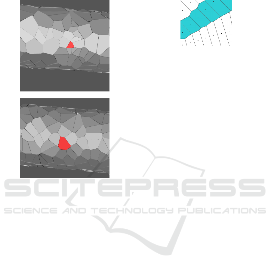
Figure 5: Tubular epithelium before (top) and after (bottom)
cell reconfiguration towards a lower energy state. Before
optimization the red cell has a volume of around 9, whereas
after reconfiguration it has a volume of 40, which is much
closer to the average cell volume of 44.
K and Λ are parameters that correspond to the elas-
tic modulus and the surface tension coefficient. The
tissue energy is simply the sum of the individual cell
energies: E(V D) :=
∑
n
i=1
E(C
i
). The function encap-
sulates that cells in an epithelium tend to have similar
volumes and compact shape, see Figure 5 for an illus-
tration. We remark that our model and the algorithm
we will present are compatible with a wide range of
energy functions, as long as the total tissue energy can
be expressed as the accumulated energy of the indi-
vidual cells.
To compute the energy of a given TφBS, we first
need to compute the 3D Voronoi diagram induced by
the cell backbones and then calculate for each individ-
ual cell its volume, its lateral area, and its perimeter
on the basal surface. In general, such a Voronoi di-
agram on n line segments has a combinatorial com-
plexity (that is, the number of vertices, edges, and
faces) in O(n
3+ε
) for ε > 0 (Koltun and Sharir, 2002).
The facets cannot simply be represented as half-space
intersections, but need to be described as an arrange-
ment of semi-algebraic functions. This also makes
area and volume computation of cells quite intricate
Figure 6: Cell (blue) represented as union of Voronoi cells
of its backbone samples.
and impractically slow already for small n. There-
fore, in practice, one usually approximates the 3D
line segment Voronoi diagrams by sampling the line
segments, computing a 3D Voronoi diagram on these
samples, and then combining the cells that are in-
duced by samples from the same backbone into one
cell. Figure 6 shows an example in 2D. A 3D Voronoi
diagram on m points has a combinatorial complexity
of O(m
2
) and its facets are convex subsets of two-
dimensional planes (Icking and Ha, 2001). Thus, cell
volumes and cell surface areas can also be computed
in O(m
2
). If we use s sample points for each of the
n cell backbones, we get m = ns and thus an overall
running time in O(n
2
s
2
). However, since we know
that a (super)cell has at most k neighbors, the number
of facets of this (super)cell decreases to O(s
2
k) and it
can be computed in O (s
2
k log(s
2
k)). As s ∈ O (1) is
a constant independent of the number of cells in the
tissue, we can compute each (super)cell in O(k log k)
or all cells in O(nk log k). Thus, especially if k is
small, the computation time is greatly reduced. Due
to Lemma 2, we know that k ∈ O(φ
2
) in a tubular
TφBS.
3.2 Metropolis–Hastings Algorithm
The Metropolis-Hastings algorithm (MH) is widely
used in cell tissue simulations, particularly for en-
ergy minimization. It provides a stochastic, itera-
tive approach to searching for lower-energy states. It
starts with some initial configuration, which can be
obtained, for example, by choosing random cell cen-
ters or backbone positions. The initial energy of this
configuration is denoted by E
0
. Then, a move is pro-
posed. Here, one selects a backbone and perturbs its
location on the apical or basal layer or both. Sub-
sequently, the energy E
′
of the resulting new con-
figuration is computed. The move might either be
accepted or rejected based on the energy difference
∆E = E
′
− E
0
. If ∆E < 0, the move decreases the en-
ergy of the tissue and is thus always accepted. How-
ever, it might also make sense to accept a move in
which ∆E ≥ 0 and the tissue energy is increased in or-
der to escape a local minimum. The acceptance prob-
ability p is usually set to p := min(1,e
−β∆E
) where
Efficient Modeling of 3D Epithelial Cell Structure Dynamics via Backbone Spreads
93

β =
1
k
B
T
with k
B
denoting the Boltzmann constant
(”energy per degree”) and T (”temperature”) being a
parameter that controls how often a system accepts
such a ”bad” move. The process is then iterated, ei-
ther with respect to the old energy state if the move
was rejected or with respect to the new energy state if
the move was accepted. The process is stopped either
after a fixed number of moves have been proposed or
if for many moves in a row now further improvement
could be found. The temperature T can be reduced
over the course of the algorithm to increase the chance
of settling in a global minimum instead of a local one
(also referred to as simulated annealing).
Oftentimes, the MH algorithm is executed in so
called steps, where in each step a move is proposed
for each backbone. The running time of a step is then
dominated by computing the tissue energy after each
proposed move. As discussed in the last subsection,
this amounts to O(nk log k) per computation, where n
is the number of backbones and k is an upper bound
on the number of neighbors per cell. Performing this
operation for each backbone, we get a running time
of O(n
2
k logk) per step, which is quite expensive.
Clearly, recomputing the tissue energy from scratch
every time a single backbone is moved is wasteful, as
only few surrounding cells might be affected. One
remedy is to use a dynamic Voronoi diagram data
structure which can be locally repaired after a change.
However, these data structures are quite intricate and
require numerically robust components, especially in
3D. Next, we discuss how to significantly decrease the
running time per step while avoiding the issues that
come with using a dynamic Voronoi data structure.
3.3 Move-Independent Set Sampling
The basic idea to improve the running time of a step is
to propose and assess multiple moves simultaneously.
Given this set of proposed moves, the new Voronoi
diagram is computed for all of them at once. Then,
instead of comparing the global tissue energy to the
previous one, we compute the local energy difference
of a move to the energy level of the surrounding cells
to adequately calculate its acceptance probability. For
this concept to work, we have to ensure that the en-
ergy of a cell is never influenced by two proposed
moves at the same time as this could distort the result.
Thus, the question is how many cells can be affected
by a single move and how one can efficiently identify
a set of moves that can be proposed simultaneously
without interference.
If backbones could move arbitrarily far, any other
cell in the tissue could be affected. But this is clearly
not possible from a biological perspective where the
tissue is expected to slowly reconfigure by small
backbone movements. Thus, we assume from now on
that backbone moves are restricted to a new position
that is still within the current cell. This implies a move
distance of at most d = 2φ in our TφBS model. For
tubular epithelia, this distance bound is evaluated on
the apical layer. Following our tubular TφBS model,
only cells fully contained in a circle of radius r =
d + 2φ = 4φ can be affected by such a move. We
now call two cells move-independent if their distance
is larger than 2r = 8φ and devise the following algo-
rithm for one MH step:
1. Partitioning. Partition the cells C
1
,. ..,C
n
into sets
S
1
,. ..,S
t
of pairwise move-independent cells.
2. Set Processing. Consider the sets one after the
other and perform the following operations:
• Compute the local energy E
L
(C
i
) for each cell
C
i
in the current set S.
• For each C
i
∈ S, propose a backbone move.
• Recompute the Voronoi diagram based on all
proposed moves.
• For each C
i
∈ S, compute its new local energy
E
′
L
(C
i
) and accept or reject the respective move
based on ∆E
L
= E
L
(C
i
) − E
′
L
(C
i
).
• Recompute the Voronoi diagram with accepted
moves only.
Clearly, if we look at one specific move of the back-
bone of cell C
i
, then the following equality should
hold: E(V D) − E
′
(V D) = E
L
(C
i
) − E
′
L
(C
i
). That
means, the global change in tissue energy induced by
the move needs to be captured by the local energy
computation. Based on our observation that only cells
within a radius of r from the original backbone posi-
tion might be affected, it suffices to compute the re-
spective node set before the move, and then evaluate
the energy of the cells in that set before the move to
get E
L
(C
i
) and after the move to get E
′
L
(C
i
). Based on
the same argument as used in the proof of Lemma 1,
we observe that there O (φ
2
) such cells in the set. Thus
the local energy computations amount to O(nφ
2
logφ)
for each step. Computing the Voronoi diagram, once
for all proposed moves and once for only accepted
moves also takes O(nφ
2
logφ) for tubular epithelia as
discussed in Section 3.1. The total running time of the
algorithm for each step is therefore in O(tnφ
2
logφ)
where t denotes the number of sets created in the par-
titioning phase.
To upper bound t, we make use of Brook’s the-
orem (Brooks, 1941). It states that a graph with n
nodes and maximum degree k has a chromatic num-
ber of at most k + 1, which means that its nodes can
be partitioned into at most k + 1 independent sets.
The partitioning can be computed in time O (nk). To
GRAPP 2025 - 20th International Conference on Computer Graphics Theory and Applications
94

use the theorem, we want to construct a graph where
the nodes represent the cells and an edge exists be-
tween any pair of cells that are not move-independent.
This can be accomplished by inducing an edge be-
tween two nodes with the respective cell backbones
having a distance of at most 2r between each other.
According to our tubular TφBS model, the maximum
degree in this graph is k ∈ O(φ
2
) and thus we can par-
tition the cells into t ∈ O(φ
2
) sets with pairwise move-
independent elements.
In total, the running time of a MH step is in
O(nφ
4
logφ) for tubular epithelia that adhere to our
model, which is essentially linear in the number of
cells. This is significantly better than the running time
of the classical implementation described in the last
subsection, where we would end up with a running
time of O(n
2
φ
2
logφ) in our tubular TφBS model. In
general TφBS model with a constant upper bound on
the maximum backbone length, the number of neigh-
bors is k ∈ O(φ
3
) and thus the total running time of
a MH step would be O (nφ
6
logφ) with our improved
algorithm.
4 SIMULATION & EVALUATION
To test the usefulness of our proposed (tubular)
TφBS model and to assess the efficiency of the
independent-set based Metropolis-Hastings (MH) al-
gorithm, called IS-MH from now on, over the classi-
cal MH algorithm for computing epithelia with low
tissue energy, we implemented the described meth-
ods in C++. Experiments were conducted on a In-
tel(R) Core(TM) i5-8250U CPU@1.60GHz with 4
cores and 32GB of RAM.
4.1 Voronoi Diagram Computation
Our model and the simulation algorithms rely on
Voronoi diagram computation for a given set of cell
backbones. As discussed in Section 3.1, we do not
compute the 3D line segment Voronoi diagram but
instead we construct a 3D point Voronoi diagram
on backbone samples and then merge the respective
Voronoi cells for each backbone. The Voronoi dia-
gram is computed via its dual, the Delaunay trian-
gulation. We use the Computational Geometry Al-
gorithms Library (The CGAL Project, 2024), in par-
ticular its robust implementation of 3D Delaunay tri-
angulations, to retrieve the cells and to compute the
properties that are important for energy minimization
(volume, area, perimeter). In all experiments, paral-
lelization is enabled.
Figure 7: Synthetically generated cell backbones.
4.2 Backbone Generator
We implemented a backbone generator for tubular ep-
ithelia. It takes the following input parameters: The
length of the tube L, the apical radius R
a
, the basal
radius R
b
, and the number of backbones n. The api-
cal and basal surface are centered around the x-axis
from x = 0 to x = L. For each backbone i = 1,... ,n,
we choose a random x-position in x
i
∈ (0,L) as well
as a random angle α
i
∈ [0, 2π) in radians. We then
construct a ray emerging from (x
i
,0, 0), which is or-
thogonal to the x-axis and has angle α to the y = 0
plane. The intersection points of the ray with the api-
cal surface and the basal surface constitute the start
and end point of the backbone segment. Figure 7
shows an example of such a backbone arrangement
with L = 80,R
a
= 10, R
b
= 20, n = 1000.
The resulting 3D Voronoi diagram when using
s = 50 samples per backbone is shown in Figure 8.
The basal and apical surface are illustrated in Figure
9. We remark that for biological simulation often-
times the number of cells n is determined based on the
choice of L, R
a
and R
b
by setting n such that the av-
erage cell volume is equal to 1. Of course, this could
be easily done in our approach as well. However, as
one of the goals of the paper is to study the running
time of the proposed energy minimization algorithm
depending on the number of cells, we keep n flexible
in our implementation.
Efficient Modeling of 3D Epithelial Cell Structure Dynamics via Backbone Spreads
95

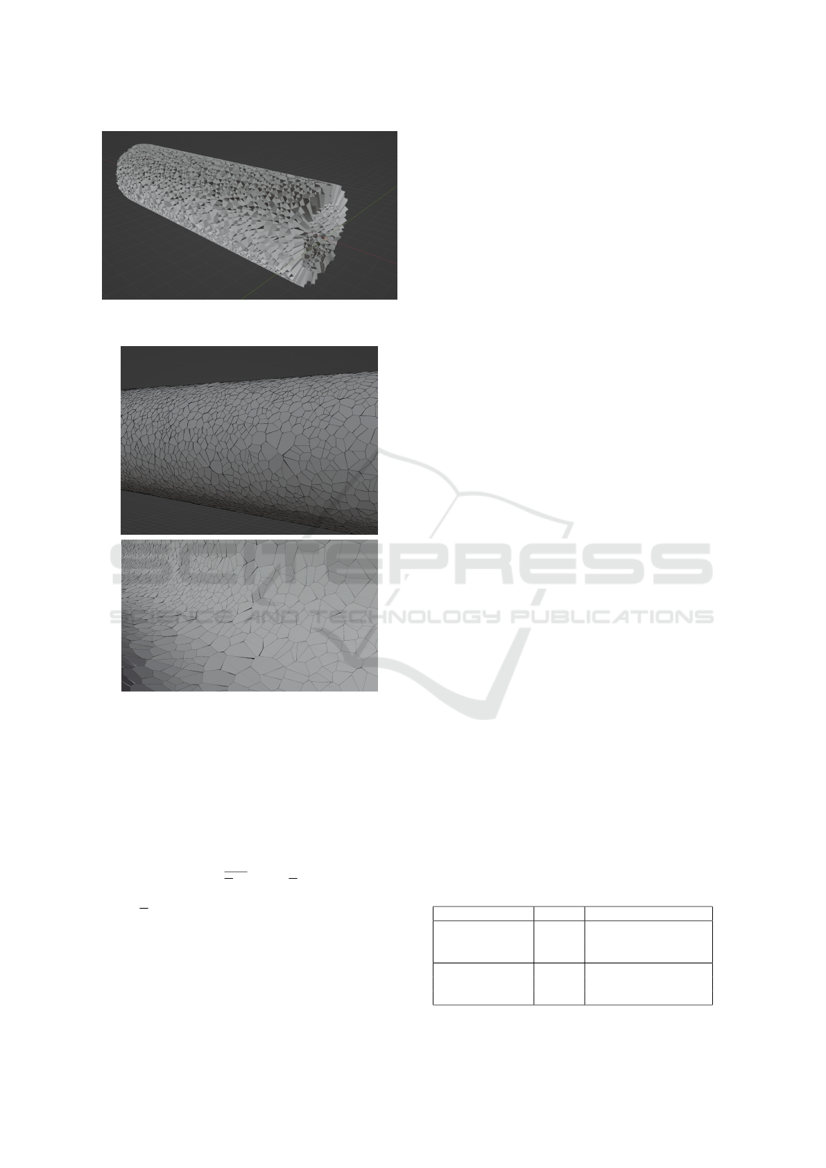
Figure 8: Voronoi cell structure for synthetically generated
cell backbones.
Figure 9: Basal surface (top) and apical surface (bottom)
of a Voronoi cell structure based on synthetically generated
cell backbones.
4.3 Energy Minimization
We use the following parameters for our implemen-
tation of the Metropolis-Hastings algorithm: For the
energy formula, we set K = 1 and Λ = 0.4. For back-
bone movements, we use an upper bound of disloca-
tion on the apical layer of
0.25
q
A/π ≈ 0.14A
1/2
where A denotes the average apical area of a cell. As
temperature value T , we use 2. If not specified other-
wise, we set L = 100,R
b
= 10,n = 500, and vary the
inner radius R
a
to study the influence of the so called
surface ratio R
b
/R
a
on the cell structure. Results are
always averaged over 10 runs.
We first investigate whether our newly proposed
IS-MH simulation algorithm is superior to the classi-
cal MH algorithm with respect to running time. Table
1 shows the running time per step for both algorithms
for different tubular configurations. In a step, a move
is proposed and evaluated for each of the n back-
bones. We observe that IS-MH is significantly faster
than MH (up to factor of 25), and the speed-up grows
for larger n. While MH has to reconstruct the whole
Voronoi diagram for each backbone individually, IS-
MH profits from processing independent sets at once.
As also shown in Table 1, the number of rounds that
IS-MH uses, which is the number of independent sets,
grows only very mildly with n. This makes sense a
larger number of cells usually also allows to identify
larger move-independent sets. It can also be seen that
for R
a
= 5 the running times and the number of rounds
are lower than for R
a
= 1. This can be explained by
the larger number of cells that are within the move-
dependent distance bound for R
a
= 1, as backbones
are longer than for R
a
= 5. However, for both R
a
and
R
b
we see an at most linear running time growth in n.
This complies with our analysis in the TφBS model
where we predicted a running time of O(nφ
4
logφ)
per step which is linear in n for constant φ. While the
initial φ-value was oftentimes large in the randomly
generated tissue (which is not expected to resemble a
real epithelium), it typically dropped quickly within
the first steps and stabilized at values between 1 and
5. For MH, we observe as expected from our analysis
a quadratic growth of the running time with increas-
ing n. It nearly quadruples when we double the num-
ber of cells from 500 to 1000 and already takes close
to an hour for the latter, while IS-MH takes less than
2 minutes. We verified that both algorithms produce
similar energy levels after the same number of steps.
We conclude that our IS-MH algorithm is preferable,
as it achieves the same result faster. In the remainder
of the paper, we always use IS-MH.
Next, we verify that our novel 3D Voronoi dia-
gram implementation of the IS-MH algorithm indeed
produces tissues of low energy and with other desired
Table 1: Running times t(MH) and t(IS-MH) for the MH
and IS-MH algorithm per step in seconds for varying R
a
and n. For IS-MH also the number of rounds r(IS-MH) is
stated, which is proportional to the number of Voronoi di-
agram computations. For MH the number of Voronoi dia-
gram computations is proportional to n.
R
a
R
b
n t(MH) t(IS-MH) r(IS-MH)
1 10 100 47.1 15.6 17
500 703.8 54.6 20
1000 2525.0 103.7 21
5 10 100 56.1 10.8 10
500 712.8 42.4 14
1000 2597.2 76.7 15
GRAPP 2025 - 20th International Conference on Computer Graphics Theory and Applications
96

0
50000
100000
150000
200000
250000
300000
350000
0 500 1000 1500 2000
tissueenergy
#rounds
R
a
=1,R
b
=10
R
a
=5,R
b
=10
Figure 10: Tissue energy over time using the IS-MH algo-
rithm on n = 500 cells.
0
20
40
60
80
100
120
140
160
180
0 50 100 150 200 250 300 350 400 450 500
cellvolume
step1
step5
step25
step50
step100
Figure 11: Cell volume distribution for R
a
= 1 in selected
steps. The x-axis reflects the cell ID after sorting them in-
creasingly by volume after the step was completed. A clear
convergence towards the average cell volume can be seen.
The final tissue has a φ value around 3.
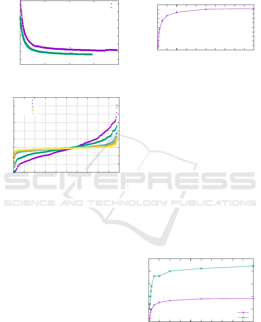
properties. Figure 10 shows the tissue energy over
time for 100 steps, for R
a
= 1 as well as R
a
= 5. We
see a steep decline in tissue energy for both setups,
especially in early rounds, followed by a slow conver-
gence towards smaller energy levels.
Figure 11 illustrates that the goal of producing
cells with roughly equal volume is also met, and
shows how the cell volume distribution changes over
time. Most cells that do not reach the equilibrium vol-
ume are close to the border of the tubular epithelium
(that is, their x-coordinates are close to 0 or L), where
it is more difficult to escape a local minimum based
on the limited move directions.
4.4 Cell Shapes & Connectivity
Finally, we want to gain insights into the connectivity
structure of the energy-minimized epithelia and study
which cell shapes emerge depending on the choice of
R
a
and R
b
. We start with an analysis of the 3D neigh-
borhoods of the cells. In (G
´
omez-G
´
alvez et al., 2021),
the so called Flintstones’ law was formulated, which
6
6.5
7
7.5
8
8.5
9
9.5
10
10.5
11
0 20 40 60 80 100 120 140 160 180 200
averagenumberof3Dneighbors
R
b
/R
a
Figure 12: Average number of neighbors for varying surface
ratios using R
b
= 10 and n = 500.
states that the average number of 3D neighbors of a
cell in a monolayer epithelium grows with the surface
ratio R
b
/R
a
following a logistic function. We con-
firmed this behavior in our implementation, as shown
in Figure 12 for a surface ratio between 1.25 and 200.
Even for a surface ratio of 1000, the average number
of neighbors stayed below 11.
Next, we take a closer look at the different types
of neighbors of a cell. With the detection of scu-
toids (G
´
omez-G
´
alvez et al., 2018), it became clear
that even in monolayer tubular epithelia with straight
backbones a cell can have different neighbors on the
apical and the basal surface. A cell is a scutoid if
at least one of its faces has a node between the api-
cal and the basal surface at which a neighbor transi-
tion occurs. It was already shown in (G
´
omez-G
´
alvez
et al., 2018) that the number of scutoids in epithelia
increases with the surface ratio. We confirmed this
result in our experiments. But we also go a step be-
yond and analyze the number of transition points per
cell that occur, see Figure 13. We observe a similar
logistic behavior for the average number of transition
points as for the average number of neighbors in Fig-
ure 12, but starting and ending at smaller values. Still,
the numbers are surprisingly large, implying that the
0
5
10
15
20
25
0 20 40 60 80 100 120 140 160 180 200
R
b
/R
a
avg.#transitionpoints
max.#transitionpoints
Figure 13: Average and maximum number of transition
points in dependency of the surface ratio. Having at least
one transition point on its faces makes a cell a scutoid. For
a surface ratio of at least 2, over 90% of cells are scutoids.
Efficient Modeling of 3D Epithelial Cell Structure Dynamics via Backbone Spreads
97

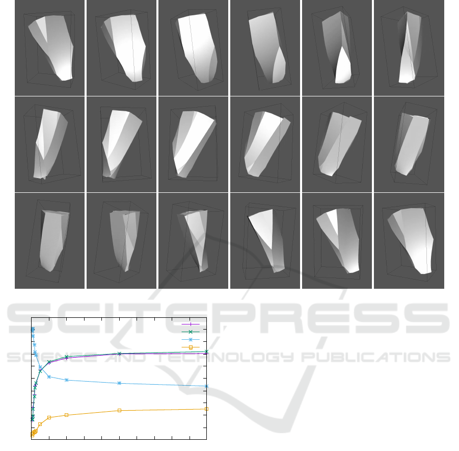
Figure 14: Complex cell structure with multiple transition points.
0
0.5
1
1.5
2
2.5
3
3.5
4
4.5
5
0 20 40 60 80 100 120 140 160 180 200
averagenumberofneighbors
R
b
/R
a
onlyapical
onlybasal
apicalandbasal
internal
Figure 15: Average number of different types of neighbors
depending on the surface ratio.
connectivity structure of cells is very complex even in
these simple tissues. Figure 14 shows an example of
a scutoid with multiple transition points.
Our study of neighborhood types revealed even
more surprising results. It has been observed that 3D
epithelium cells exhibit the following types of neigh-
bors, based on whether the cells touch:
1. On both, the apical and basal surface.
2. On the apical surface but not on the basal surface.
3. On the basal surface but not on the apical surface.
A non-scutoid can only have neighbors of type 1.
However, we discovered that scutoids might not only
have neighbors of the three types specified above, but
also neighbors that only have a common feature with
a cell between the apical and the basal surface but
not on either of the surfaces. We call this an inter-
nal neighbor. Figure 15 shows the distribution of the
different types of neighbors.
We observe an interesting trend. For small surface
ratio, almost all neighbors are neighbors on both the
apical and the basal surface, which complies with the
observation that there are few to no scutoids in these
tissues. However, for growing surface ratio, their
number shrinks drastically and is then overtaken by
the number of only apical and only basal neighbors,
respectively. The number of only apical or only basal
neighbors is almost identical on average. Both in-
crease similarly with growing surface ratio. But what
also increases, is the number of internal neighbors.
For a surface ratio of 10, already 65% of cells had at
least one internal neighbor. While the average number
of internal neighbors does not go substantially above
one, it was not clear before that the tubular epithelium
structure would even allow for such neighbors. Thus
it is interesting to observe their natural emergence in
our implementation. Figure 16 shows the 3D config-
uration of two cells that are internal neighbors.
GRAPP 2025 - 20th International Conference on Computer Graphics Theory and Applications
98

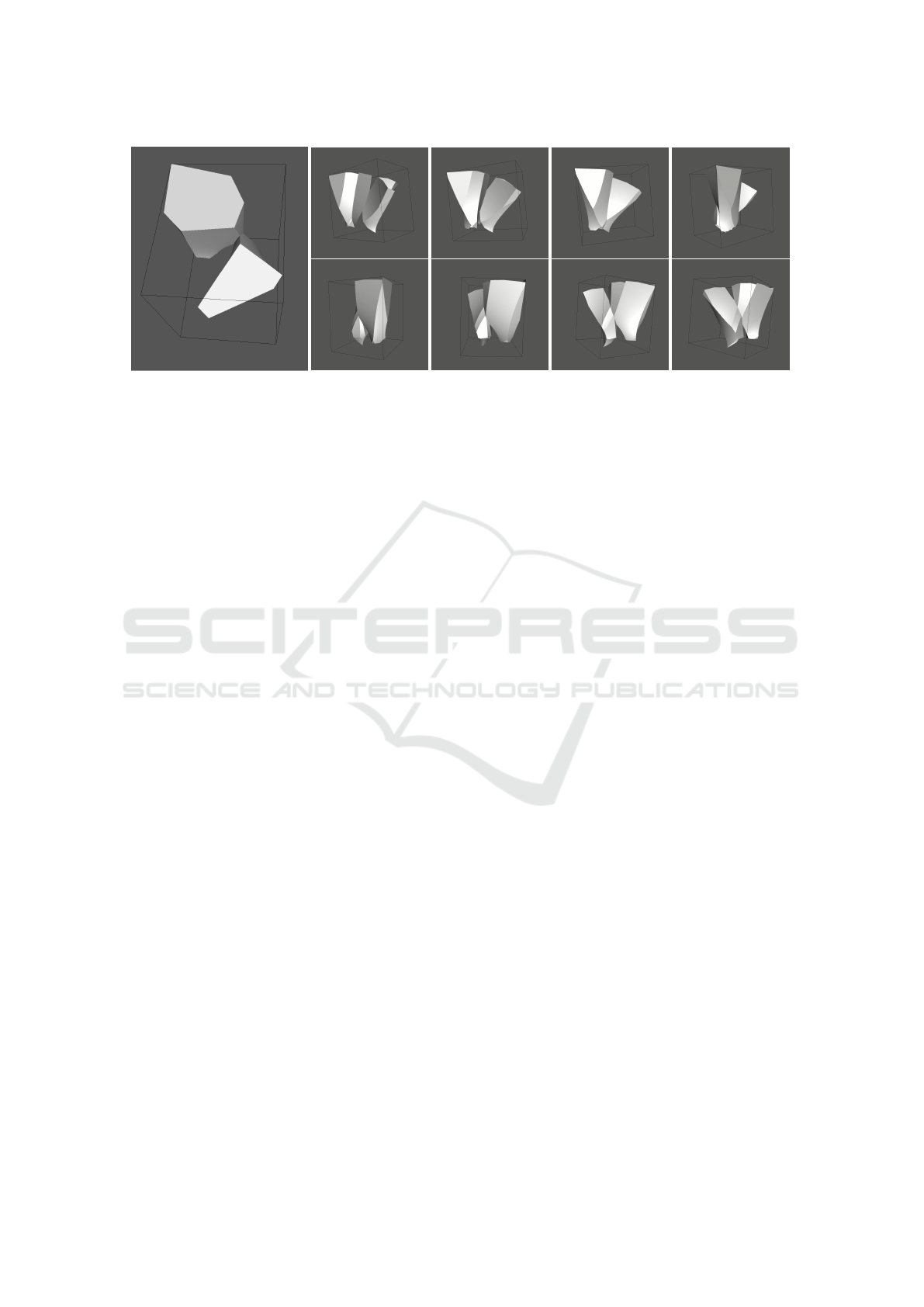
Figure 16: Two cells touching in the interior without being apical or basal neighbors. Left: view on the apical surface; Right:
different views of the two cells.
5 CONCLUSIONS AND FUTURE
WORK
We have proposed a new 3D cell-center model for
monolayer epithelia associated with geometric con-
straints modulated by a parameter φ, which is ex-
pected to be small in real tissues. We proved that in
tubular epithelia the maximum neighborhood size of
a cell can be upper bounded in terms of φ. This al-
lowed us to propose a new variant of the Metropolis-
Hastings algorithm for tissue energy minimization,
which is provably fast for small φ and also showed
superior performance compared to the classical ver-
sion in our experimental evaluation.
Furthermore, we studied the shape and connectiv-
ity of the cells and observed that surprisingly complex
structures emerge, as scutoids with a large number of
transition points as well as internal neighborhood re-
lations. It will be interesting to see whether similar
structures are formed in other types of epithelia, for
example in spheroidal epithelia as studied in (G
´
omez-
G
´
alvez et al., 2018).
It has been observed that in spite of smooth api-
cal and basal surfaces, in some settings, cells might
assume highly irregular shapes, which were named
punakoids (Iber and Vetter, 2022). If a cell’s vol-
ume is to be represented by a suitable Voronoi tesse-
lation of space with respect to a cell center, straight
cell backbones do not seem to be able to generate
such punakoids. Our approach of representing the
cell backbone by point samples in principle allows
for non-straight backbones. In future work, we aim
at identifying realistic constraints on the flexibility of
cell backbones in order to be able to model even more
cell shapes occurring in nature.
Our current implementation of the 3D Voronoi di-
agram is based on the exact geometric computation
paradigm, which – while providing immunity to ro-
bustness issues – is quite time consuming. Alterna-
tively one might consider GPU-based Voronoi con-
structions like (Ray et al., 2018) which promise faster
iterations for the (IS-)MH algorithm.
ACKNOWLEDGEMENTS
This work was initiated during the Leiden Workshop
”Beyond Abstract Measures: Geometry and Compu-
tation” which took place in 2022 at the Lorentz Cen-
ter in Leiden (Lorentz Center, 2022). Subsequently,
the research was supported by the DFG grants STO
1114/5-1 and FU 700/5-1.
J.B. furthermore acknowledges support
from the grant PID2022-137436NB-I00 and
the research network RED2022-134573-T
funded by ‘Ministerio de Ciencia e Innovacion’
(MCIN/AEI/10.13039/501100011033) and by ERDF
‘A way of making Europe’ by the E.U. Additional
support to J.B. was provided by the E.U. COST
action CA22153 ‘European Curvature and Biology
Network’ (EuroCurvoBioNet).
REFERENCES
Alt, H. and Schwarzkopf, O. (1995). The voronoi diagram
of curved objects. In Proceedings of the eleventh an-
nual symposium on Computational geometry, pages
89–97.
Alt, S., Ganguly, P., and Salbreux, G. (2017). Vertex mod-
els: from cell mechanics to tissue morphogenesis.
Philosophical Transactions of the Royal Society B: Bi-
ological Sciences, 372(1720):20150520.
Brooks, R. L. (1941). On colouring the nodes of a net-
work. In Mathematical Proceedings of the Cambridge
Efficient Modeling of 3D Epithelial Cell Structure Dynamics via Backbone Spreads
99

Philosophical Society, volume 37(2), pages 194–197.
Cambridge University Press.
Burnikel, C., Mehlhorn, K., and Schirra, S. (1994a). How to
compute the voronoi diagram of line segments: Theo-
retical and experimental results. In ESA, volume 855
of Lecture Notes in Computer Science, pages 227–
239. Springer.
Burnikel, C., Mehlhorn, K., and Schirra, S. (1994b).
How to compute the voronoi diagram of line seg-
ments: Theoretical and experimental results. In Al-
gorithms—ESA’94: Second Annual European Sym-
posium Utrecht, The Netherlands, September 26–28,
1994 Proceedings 2, pages 227–239. Springer.
Carpenter, L. C., P
´
erez-Verdugo, F., and Banerjee, S.
(2024). Mechanical control of cell proliferation pat-
terns in growing epithelial monolayers. Biophysical
Journal, 123(7):909–919.
G
´
omez-G
´
alvez, P., Vicente-Munuera, P., Anbari, S., Buc-
eta, J., and Escudero, L. M. (2021). The complex
three-dimensional organization of epithelial tissues.
Development, 148(1):dev195669.
G
´
omez-G
´
alvez, P., Vicente-Munuera, P., Anbari, S., Tagua,
A., Gordillo-V
´
azquez, C., Andr
´
es-San Rom
´
an, J. A.,
Franco-Barranco, D., Palacios, A. M., Velasco, A.,
Capit
´
an-Agudo, C., et al. (2022). A quantitative bio-
physical principle to explain the 3d cellular connectiv-
ity in curved epithelia. Cell Systems, 13(8):631–643.
G
´
omez-G
´
alvez, P., Vicente-Munuera, P., Tagua, A., Forja,
C., Castro, A. M., Letr
´
an, M., Valencia-Exp
´
osito, A.,
Grima, C., Berm
´
udez-Gallardo, M., Serrano-P
´
erez-
Higueras,
´
O., et al. (2018). Scutoids are a geometri-
cal solution to three-dimensional packing of epithelia.
Nature communications, 9(1):1–14.
Held, M. (2001). Vroni: An engineering approach to the re-
liable and efficient computation of voronoi diagrams
of points and line segments. Computational Geome-
try, 18(2):95–123.
Honda, H., Tanemura, M., and Nagai, T. (2004). A three-
dimensional vertex dynamics cell model of space-
filling polyhedra simulating cell behavior in a cell ag-
gregate. Journal of theoretical biology, 226(4):439–
453.
Iber, D. and Vetter, R. (2022). 3d organisation of cells
in pseudostratified epithelia. Frontiers in Physics,
10:898160.
Icking, C. and Ha, L. (2001). A tight bound for the com-
plexity of voroni diagrams under polyhedral convex
distance functions in 3d. In Proceedings of the thirty-
third annual ACM symposium on Theory of comput-
ing, pages 316–321.
Koltun, V. and Sharir, M. (2002). Three dimensional eu-
clidean voronoi diagrams of lines with a fixed number
of orientations. In Proceedings of the eighteenth an-
nual symposium on Computational geometry, pages
217–226.
Lau, C., Kalantari, B., Batts, K., Ferrell, L., Nyberg, S.,
Graham, R., and Moreira, R. K. (2021). The voronoi
theory of the normal liver lobular architecture and its
applicability in hepatic zonation. Scientific reports,
11(1):9343.
Ledoux, H. (2007). Computing the 3d voronoi diagram
robustly: An easy explanation. In 4th International
Symposium on Voronoi Diagrams in Science and En-
gineering (ISVD 2007), pages 117–129. IEEE.
Ledoux, H. (2008). The kinetic 3d voronoi diagram: A
tool for simulating environmental processes. In Ad-
vances in 3D Geoinformation Systems, pages 361–
380. Springer.
Lorentz Center (2022). Beyond abstract measures: geome-
try and computation. https://www.lorentzcenter.nl.
Man
´
ak, M. and Kolingerov
´
a, I. (2010). Fast discovery of
voronoi vertices in the construction of voronoi dia-
gram of 3d balls. In 2010 International Symposium on
Voronoi Diagrams in Science and Engineering, pages
95–104. IEEE.
Markovi
ˇ
c, R., Marhl, M., and Gosak, M. (2020). Mechani-
cal cell-to-cell interactions as a regulator of topologi-
cal defects in planar cell polarity patterns in epithelial
tissues. Frontiers in Materials, 7:264.
Mayya, N. and Rajan, V. (1996). Voronoi diagrams of poly-
gons: A framework for shape representation. Journal
of Mathematical Imaging and Vision, 6:355–378.
Mimura, T. and Inoue, Y. (2023). Cell-center-based
model for simulating three-dimensional monolayer
tissue deformation. Journal of Theoretical Biology,
571:111560.
Neagu, A., Mironov, V., Kosztin, I., Barz, B., Neagu,
M., Moreno-Rodriguez, R. A., Markwald, R. R.,
and Forgacs, G. (2010). Computational modeling of
epithelial–mesenchymal transformations. Biosystems,
100(1):23–30.
Okuda, S., Inoue, Y., Eiraku, M., Sasai, Y., and Adachi,
T. (2013). Reversible network reconnection model
for simulating large deformation in dynamic tis-
sue morphogenesis. Biomechanics and modeling in
mechanobiology, 12:627–644.
R. Noppe, A., Roberts, A. P., Yap, A. S., Gomez, G. A.,
and Neufeld, Z. (2015). Modelling wound closure in
an epithelial cell sheet using the cellular potts model.
Integrative Biology, 7(10):1253–1264.
Ray, N., Sokolov, D., Lefebvre, S., and L
´
evy, B. (2018).
Meshless voronoi on the gpu. ACM Trans. Graph.,
37(6).
Roos, T. (1993). Voronoi diagrams over dynamic scenes.
Discrete Applied Mathematics, 43(3):243–259.
The CGAL Project (2024). CGAL User and Reference Man-
ual. CGAL Editorial Board, 6.0 edition.
GRAPP 2025 - 20th International Conference on Computer Graphics Theory and Applications
100