
A Two-Phase Safe Reinforcement Learning Framework for Finding the
Safe Policy Space
A. J. Westley
a
and Gavin Rens
b
Computer Science Division, Stellenbosch University, Stellenbosch, South Africa
Keywords:
Safe Reinforcement Learning, Constrained Markov Decision Processes, Safe Policy Space, Violation Measure.
Abstract:
As reinforcement learning (RL) expands into safety-critical domains, ensuring agent adherence to safety con-
straints becomes crucial. This paper introduces a two-phase approach to safe RL, Violation-Guided Identifi-
cation of Safety(ViGIS), which firstidentifies a safe policy space and then performs standard RL within this
space. We present two variants: ViGIS-P, which precalculates the safe policy space given a known transition
function, and ViGIS-L, which learns the safe policy space through exploration. We evaluate ViGIS in three
environments: a multi-constraint taxi world, a deterministic bank robber game, and a continuous cart-pole
problem. Results show that both variants significantly reduce constraint violations compared to standard and
β-pessimistic Q-learning, sometimes at the cost of achieving a lower average reward. ViGIS-L consistently
outperforms ViGIS-P in the taxi world, especially as constraints increase. In the bank robber environment,
both achieve perfect safety. A Deep Q-Network (DQN) implementation of ViGIS-L in the cart-pole domain
reduces violations compared to a standard DQN. This research contributes to safe RL by providing a flexi-
ble framework for incorporating safety constraints into the RL process. The two-phase approach allows for
clear separation between safety consideration and task optimization, potentially easing application in various
safety-critical domains.
1 INTRODUCTION
Reinforcement learning (RL) is a subfield of ma-
chine learning wherein an autonomous agent explores
a given environment with the goal of learning how to
complete a task. RL has seen a large increase in pop-
ularity over the last decade due to its use in the fields
of robotics as well as video game and board game AI
(Silver et al., 2016). RL has a key advantage: pro-
grammers are not required to specify how the agent
completes its task (Kaelbling et al., 1996). Instead,
they need only design a system that rewards the agent
for good actions and punishes it for bad actions; a
punishment can be seen as a negative reward.
With RL being applied to an ever-increasing array
of problems, safety has become a growing concern.
Regular RL models seek only to maximise their re-
wards, and thus provide no guarantees that they will
take safety into account when learning or performing
tasks (Srinivasan et al., 2020). This is often not an
issue, but in environments where safety is paramount
the agent should also endeavour to stick within the
a
https://orcid.org/0009-0009-5497-1375
b
https://orcid.org/0000-0003-2950-9962
given safety constraints. For example, if you are
building a self-driving car, then crashing even once
could result in severe damage to the car. Under stan-
dard RL regimes, the only way for the car to know
how not to crash would be to receive negative rewards
for crashing, which requires the car to crash. On the
other hand, if the car seeks only to take the safest ac-
tion, then the safest action would likely be to remain
still and never leave its parking space. In this case, the
car will never complete its task. This underscores the
need for effective safe RL techniques.
Safe RL is a subtopic of RL wherein algorithms
endeavour to keep a balance between safety and per-
formance across a wide array of problem spaces
(Garc
´
ıa and Fern
´
andez, 2015). Designing algorithms
that can strike this balance is a difficult task, and the
necessary approach is often dependent on the problem
at hand. To approach these problems various tech-
niques have emerged, including constraint optimisa-
tion, model-based RL, providing predefined safety
rules, or modifying the reward by heavily penalising
unsafe actions.
This research proposes a two-phase RL approach
designed to ensure safety during both the learning
Westley, A. J. and Rens, G.
A Two-Phase Safe Reinforcement Learning Framework for Finding the Safe Policy Space.
DOI: 10.5220/0013151600003890
In Proceedings of the 17th International Conference on Agents and Artificial Intelligence (ICAART 2025) - Volume 2, pages 275-285
ISBN: 978-989-758-737-5; ISSN: 2184-433X
Copyright © 2025 by Paper published under CC license (CC BY-NC-ND 4.0)
275

and implementation phases. The algorithm, called
Violation-Guided Identification of Safety (ViGIS),
first learns a safe policy space, then performs stan-
dard RL within the predetermined safe policy space.
The process of learning the safe policy space is based
on Constrained Markov Decision Processes (Altman,
1999), using a violation measure (Nana, 2023) to
quantify each policy’s safety. There are two main
novelties to ViGIS: it is agnostic of the underlying RL
algorithm used during phase-two, and violation toler-
ances to be specified for each constraint, thus forming
a preferential order between the constraints. From
these constraints, the agent can precompute or learn
the safe policy space in silico, providing a safety boot-
strap for the goal-learning process. With this in mind,
we address the following questions: How can we an-
alytically determine the safe policy space when the
transition function and constraints are given? How
does analytically determining the safe policy space
perform compared to learning it empirically? How
does learning only within the safe policy space affect
an agent’s performance?
The rest of this paper is structured as follows: Sec-
tion 2 sets out the necessary theoretical background
for the paper by explaining Markov Decision Pro-
cesses and Constrained Markov Decision Processes,
then introducing the notion of policies and safe pol-
icy spaces. Section 3 provides an overview of re-
cent safe RL approaches, with a particular focus on
a Master’s thesis, which serves as inspiration to the
research presented in this paper (Nana, 2023). In Sec-
tion 4, the two-phase algorithm is introduced, its un-
derlying mathematics is explained, and a pseudocode
is provided. Section 5 describes the various testing
environments along with their respective safety con-
straints and success criteria, after which it evaluates
the algorithm in these testing environments. The two-
phase agent is compared to a regular RL agent to as-
sess its safety, as well as its overall performance and
efficiency. To end off, Section 6 summarises the work
done in this paper and provides some closing remarks
on potential extensions of the work.
2 BACKGROUND
2.1 Markov Decision Processes
A Markov Decision Process (MDP) is a framework
for modelling fully observable, stochastic, sequen-
tial decision problems. In reinforcement learning,
MDPs are used to model interactions between an
agent and its environment. MDPs have Markovian
state transitions, meaning the next state depends only
on the current state (and action). Constraints can be
added to a standard MDP, making it a constrained
MDP (CMDP). Throughout this paper, unless explic-
itly stated otherwise, MDP refers to an unconstrained
MDP.
2.1.1 Unconstrained MDPs
An MDP can be defined by the tuple ⟨S, A, T, R⟩
(Russell and Norvig, 2010):
• S is the set of all states which exist within the
MDP – the state space.
• A is the set of all actions which can be performed
in each state – the action space.
• T : S × A → Distr(S) is the transition function
which gives the probabilities of transitioning from
some state s to another state s
′
when an action a is
performed. For a particular s, s
′
and a, this func-
tion is defined as:
P
a
(s, s
′
) = P(s
t+1
= s
′
|s
t
= s, a
t
= a) (2.1)
• R : S × A → R is the reward function that cal-
culates the value of each state-action pair. This
expresses the instantaneous benefit of performing
action a in state s. The reward gained at a partic-
ular time t is notated as R
t
.
The goal of solving an MDP is to find a sequence of
actions which maximise the total reward gained ac-
cording to R.
2.1.2 Constrained MDPs
In environments where some states are undesirable,
we can extend the MDP framework by adding con-
straints, leading to a CMDP. In this case, the tuple be-
comes ⟨S, A, T, R, C⟩ (Altman, 1999). All elements
of the tuple remain the same, but for the addition of
C, which is expressed as
{c
i
: S × A → R|i = 1, . . . , k} (2.2)
where k is the number of constraints in the system
(Ge et al., 2019). C specifies which states in the state
space are not safe. It can reduce the state and action
spaces that may be explored in the MDP or it can al-
ter the reward function directly. With C added to the
MDP framework the objective is no longer to only
maximise the reward gained according to R, but to
also abide by the constraints specified by C. These
constraints can be set for various reasons, but in this
study they will mostly be safety constraints. Fig. 1
shows how CMPDs fit into the context of RL.
2.2 Policy and Safe Policy Space
The goal of any RL algorithm is for the agent to find
the best actions in order to reach a given objective.
ICAART 2025 - 17th International Conference on Agents and Artificial Intelligence
276
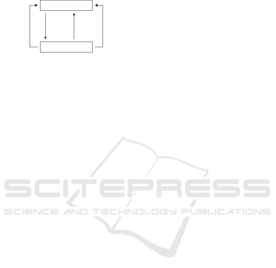
Agent
Environment
(1)
Feasible
actions
(according
to constraints)
(2)
Action a
t
(3)
Reward r
t
(4)
State s
t+1
(according to
transition
function)
Figure 1: An abstract representation of a CMDP through
the lens of reinforcement learning.
These actions are usually expressed in the form of a
policy. A policy is a set of state-action pairs which
indicates the best action to perform from any given
state.
The set of all possible policies for a particular
problem is called the policy space of the problem. The
policy space grows exponentially in size with the ac-
tion and state spaces, and thus can become enormous
for discrete problems, and even infinite for continu-
ous problems (Mutti et al., 2022). All policies, even
those which do not complete the goal are included in
the policy space. In safe RL, we are not interested
in policies which would violate the safety constraints,
so we can rather look at the subset of policies which
adhere to these constraints. This policy subspace is
called the safe policy space.
3 RELATED WORKS
3.1 Safe Reinforcement Learning
Safe RL has existed as a topic for over a decade and
thus there has been a significant amount of research
done in the field (Garc
´
ıa and Fern
´
andez, 2012; Gas-
kett, 2003; Driessens and D
ˇ
zeroski, 2004; Gerami-
fard et al., 2011). In this part, we summarise and
discuss different safe RL approaches with reference
to a taxonomy proposed by Garc
´
ıa and Fern
´
andez
(2015). According to this taxonomy, there are two
overarching categories of Safe RL techniques, which
entail modifying either the optimization criterion or
the exploration process. We end off the section by
discussing where ViGIS fits into the field of safe RL.
3.1.1 Optimization Criterion
One over-arching approach to safe RL is to directly
modify the optimization criterion. The three most
common modifications are: worst case, risk-sensitive,
and constrained criterion.
A worst case criterion is one which aims to find
a policy which maximizes the expected reward in the
worst-case scenario, when there is uncertainty in the
environment. Gaskett (2003) addressed the stochas-
tic environment problem by proposing a modified Q-
Learning algorithm, called β-pessimistic Q-Learning.
β-pessimistic Q-Learning aims to strike a balance be-
tween maximising the reward of the worst case and
the best case. It does this using the following update
equation:
Q
β
(s, a) ← (1 − α)Q
β
(s, a) + α
h
R
t+1
+ γ
(1 − β
p
)max
a
′
∈A
Q(s
′
, a
′
) + β
p
min
a
′
∈A
Q(s
′
, a
′
)
i
,
(3.1)
where β
p
∈ [0, 1] is the hyperparameter which tunes
the agent’s consideration of risk. Larger β
p
values
make the agent more averse to risk.
Risk-sensitive criteria contain a hyperparameter
which tunes the agent’s consideration of risk. This
hyperparameter can be tuned by the programmer to
specify a subjective balance between risk and reward.
Inside the criterion, the hyperparameter is usually in-
corporated into an exponential function, or a weighted
sum of risk and reward.
A constrained criterion is similar to a typical con-
strained optimization problem, as the goal is to find
the optimal solution which satisfies a given set of con-
straints. As per the name, these criteria usually take
the form of a CMDP.
3.1.2 Exploration Process
The other approach is to modify the exploration pro-
cess directly. This is usually done by providing the
agent with external knowledge in the form of: initial
knowledge, or teacher advice.
Providing the agent with initial knowledge gives
it a leg-up at the beginning of the learning process.
The agent can use this knowledge to avoid some un-
desirable parts of the state space completely, which
reduces the size of the state space which needs to be
explored.
An agent can also be provided with teacher advice
during the learning process. This approach requires
the presence of some form of teacher: human or oth-
erwise. The teacher can then provide the agent with
advice whenever the agent asks or the teacher deems
it necessary. An advantage of this approach is that it
allows the teacher to manually prevent the agent from
making choices which could have dangerous conse-
quences.
3.1.3 Model-Based Look-Ahead Approaches
In addition to the approaches discussed above, there
have been some promising model-based algorithms to
A Two-Phase Safe Reinforcement Learning Framework for Finding the Safe Policy Space
277

preempt any constraint violations. These approaches
are the most similar to ViGIS, but ViGIS differs from
these because it functions as a framework wherein
other RL methods can be used, and it finds the safe
policy space of a problem domain, rather than em-
ploying a direct look-ahead strategy. One example
that has shown promise is the notion of probabilistic
shields (Yang et al., 2023). This method involves log-
ically modeling the environment and its constraints,
then using this model to determine the respective
probabilities of violating these constraints. An al-
ternative to shielding is to use model-based rollouts
to predict future violations. This approach, called
Safe Model-Based Policy Optimization (SMBPO),
was presented by (Thomas et al., 2024) SMBPO uses
Gaussian dynamics models during rollouts to assess
the safety of each trajectory, then heavily penalises
trajectories that are deemed unsafe. In addition to the
reasons already discussed, SMBPO also differs from
ViGIS in that ViGIS does not make use of any roll-
out scheme. One last notable approach is Safe Upper
Confidence Bound Value Iteration (SUCBVI), pro-
posed by (Xiong et al., 2023). SUCBVI is an exten-
sion of UCBVI to incorporate step-wise constraints.
SUCBVI is similar to ViGIS in its use of step-wise
constraint avoidance as opposed to long-term viola-
tion minimisation. It also bears similarity to ViGIS
due to it operating as a framework, rather than a stand-
alone algorithm.
3.2 Violation Measure
ViGIS makes use of the violation measure that was
formulated by Nana (2023). This violation measure
is centred around the idea that, in many problems, it
may not be possible to know with certainty whether
some state-action pairs will lead to a safety violation.
To deal with these problems it makes sense to model
risk as the probability that performing action a in state
s will lead to a dangerous situation. In the violation
measure formulation, a tolerance is specified for each
constraint of how high this probability can be, which
allows the weight of each constraint to be carefully
tuned. The violation measure function is expressed as
V
C
(s, a) =
1
|C|
∑
(c
i
,p
i
)∈C
max{0,
ˆ
P(c
i
|s, a) − p
i
} (3.2)
where V
C
refers to the violation measure as per con-
straint set C, |C| is the cardinality of that set,
ˆ
P(c
i
|s, a)
is the probability that constraint c
i
will be violated by
performing action a in state s, and p
i
is the tolerance
threshold for constraint c
i
. For example, if the taxi-
routing system might be more willing to route the taxi
through a storm than an area with a high crime rate,
in which case the constraint set would be:
C = {(c
crime
, 0.1), (c
storm
, 0.5)}. (3.3)
Since V
C
is essentially the average of a set of
probabilities, it will always produce a real number
between zero and one. The violation measure, it-
self, is a constrained criterion that expresses the aver-
age violation probability across all states that can be
reached from the current state. Nana applies the viola-
tion function in two different ways: inside the reward
function to modify the reward function, and outside
the reward function as a risk-sensitive criterion. The
risk sensitive criterion leads to the following expres-
sion for the optimal policy:
π
∗
(s) = argmax
a∈A
[Q(s, a) − βU (s, a)] (3.4)
where β is the tuning hyperparameter and U(s, a) is
the U-function, which is formulated similarly to the
Q-function. The only difference with the U-function
is that instead of maximising the reward function, it
aims to minimize the violation measure according to
the following update equation.
U(s, a) ← (1 − α)U (s, a)
+ α(V
C
(s, a) + γ · min
a
′
∈A
U(s
′
, a
′
)).
(3.5)
4 THE TWO-PHASE
ALGORITHM
In Section 3.2, the violation measure is used to modify
the optimization criterion, but this is not the only way
it can be used. Here we propose a two-phase algo-
rithm, ViGIS, that uses the violation measure to mod-
ify the exploration process by providing initial knowl-
edge. ViGIS works as follows:
1. The violation function is used to find the prob-
lem’s safe policy space.
2. RL is performed within the safe policy space.
We also describe some variants of ViGIS and end off
the section by summarising the base algorithm and
these variants.
4.1 Setup
Before we derive the algorithm, it is important to lay
out any necessary assumptions, and prior knowledge.
ViGIS assumes the existence of a violation delta func-
tion which is expressed as follows:
δ(c, s) =
(
1, s violates constraint c
0, otherwise
(4.1)
ICAART 2025 - 17th International Conference on Agents and Artificial Intelligence
278

This violation delta function expresses whether or not
a state s violates a particular constraint c.
ViGIS also assumes that the following compo-
nents of a CMDP are present and known: the state
space S, the action space A, a reward function R, and
a set of constraints C. There are two different ap-
proaches to this algorithm, one of which assumes that
the transition function T = P(s
′
|s, a) is known. If T is
unknown in this case, it can be learnt using RL tech-
niques or estimated by Monte Carlo simulation.
4.2 Phase One: Finding the Safe Policy
Space
To find the safe policy space, we will explore two dif-
ferent approaches: we can precalculate the safety of
every state-action pair in the policy space, or we can
learn it using RL itself.
4.2.1 ViGIS-P: Precalculating the Safe Policy
Space
ViGIS-P is the base form of the ViGIS algorithm,
wherein the agent precalculates the violation measure
for every possible state-action pair. This algorithm
defines the safe policy space in terms of the viola-
tion function discussed in Section 3.2. If Π is the pol-
icy space of a particular problem, then the safe policy
space is the set of all policies, π ∈ Π, in which all
state-action pairs have a violation measure that falls
below some predefined violation threshold β. This
threshold functions as a hyperparameter that can be
used to tune the agent’s overall aversion to risk. For-
mally, the safe policy space can be defined as:
Π
safe
={π ∈ Π|s ∈ S, a ∈ A,
(s, a) ∈ π,V
C
(s, a) ≤ β}
(4.2)
where Π
safe
is the safe policy space, (s, a) is a state-
action pair in policy π, and β ∈ [0, 1] is the violation
threshold. This is not the full picture, however, as V
C
must still be calculated.
There are three main parameters in the violation
function
1
: C, p
i
, and
ˆ
P(c
i
|s, a). Since C and p
i
are both assumed to be known, the only unknown is
ˆ
P(c
i
|s, a). Let us then redefine
ˆ
P(c
i
|s, a) in terms of
what is already known.
Theorem 1. Let S be the state space of an MDP,
δ(c, s) = P(c|s) be a violation delta function, and
P(s
′
|s, a) be the transition function, then the proba-
bility of violating constraint c by performing action a
in state s,
ˆ
P(c|s, a), can be expressed as
ˆ
P(c|s, a) =
∑
s
′
∈S
P(s
′
|s, a)δ(c, s
′
). (4.3)
1
see Equation 3.2
Proof.
ˆ
P(c|s, a) =
∑
s
′
∈S
P(c, s
′
|s, a)
=
∑
s
′
∈S
P(c|s
′
, s, a)P(s
′
|s, a)
c is independent of s and a given s
′
.
∴
ˆ
P(c|s, a) =
∑
s
′
∈S
P(c|s
′
)P(s
′
|s, a)
=
∑
s
′
∈S
P(s
′
|s, a)δ(c, s
′
)
Algorithm 1: Determine whether or not the state-action pair
(s, a) is safe.
Function IS SAFE(s, a, C, β):
c ← set of constraints in C
p ← set of tolerance thresholds in C
V
C
← 0
for i = 1 to |C| do
ˆ
P ← 0
forall s
′
in S do
ˆ
P ←
ˆ
P + P(s
′
|s, a) · δ(c[i], s
′
)
end
V
C
← V
C
+ max (0,
ˆ
P − p[i])
end
V
C
←
1
|C|
·V
C
if V
C
≤ β then
return true
else
return false
end
end
Algorithm 2: Determine the safe policy space.
Function POLICY SPACE(S, A, C, β):
Π
safe
← |S| × |A| boolean matrix
forall s in S do
forall a in A do
Π
safe
[s][a] ← IS SAFE(s, a, C, β)
end
end
return Π
safe
end
Algorithm 1 shows how a single state-action pair
can be evaluated as either safe or unsafe, using The-
orem 1. Using this, Algorithm 2 determines the safe
policy space by evaluating every possible state-action
pair. As shown in Algorithm 2, a Boolean matrix is
used to store whether a state-action pair is safe or not,
but it may also be useful to store the violation mea-
sures themselves instead. If we store a V
C
table, its
values can still be compared to our β parameter on
A Two-Phase Safe Reinforcement Learning Framework for Finding the Safe Policy Space
279

the fly to determine a state’s safety, while also allow-
ing the potential for comparing or updating these val-
ues during the agent’s learning phase. This will be
explored further in Section 4.3.
4.2.2 ViGIS-L: Learning the Safe Policy Space
ViGIS-L is an alternative approach to finding the safe
policy space, where the safe policy space is found us-
ing RL, rather than a full precalculation. This would
be akin to training an agent in a safety simulation be-
fore transfering it to a physical robot to learn its task.
In this regime, we learn the safe policy space using a
recursive policy space update function which resem-
bles that of Q-Learning:
ˆ
V
C
(s, a) ← (1 − α)
ˆ
V
C
(s, a)
+ α(V
C
(s, a) + η · min
a
′
∈A
ˆ
V
C
(s
′
, a
′
)),
(4.4)
where η is a discount factor. Instead of maximising
rewards like typical Q-Learning, this method learns
the
ˆ
V (s, a) values by minimising violations. Since Q-
Learning is model-free, this method does not require
a transition function to operate. This is advantageous,
because in most stochastic environments the transi-
tion function is not known beforehand. To exclude the
transition function from V
C
(s, a), we replace it with
the following:
W (s
′
) =
1
|C|
∑
(c
i
,p
i
)∈C
max
0, δ(c, s
′
) − p
i
. (4.5)
This formulation expresses the violation measure of a
single given state s
′
. The resulting update equation,
using W(s
′
), is
ˆ
V
C
(s, a) ← (1 − α)
ˆ
V
C
(s, a)
+ α(W (s
′
) + η · min
a
′
∈A
ˆ
V
C
(s
′
, a
′
)).
(4.6)
In this approach, an agent in state s takes an ac-
tion a and arrives at subsequent state s
′
, then updates
ˆ
V
C
(s, a) based on the perceived level of violation in
state s
′
. This formulation is valid because, in the
limit of infinite exploration, the agent will make all
state transitions with their relative frequencies. This
approach still requires violations on the part of the
agent. This being said, this phase can be performed
in silico before the agent is transferred to the target
environment where learning the task is likely to be
more accurate. Just like with reward-based RL, this
approach should not only learn if a state-action pair
will cause an immediate safety violation, but also if
it may cause a violation further into the future. This
will result in the RL approach learning different vi-
olation values to the precalculation method. More
specifically, the
ˆ
V
C
values could exceed one. In this
case,
ˆ
V
C
can no longer be treated like probabilities.
This means that either beta may need to be tuned to a
value greater than one, or
ˆ
V
C
must be normalised. In
this paper, we normalise
ˆ
V
C
empirically for all tabu-
lar Q-Learning agents, and leave it unnormalised for
the Deep Q-Network agent. There is likely an analyt-
ical approach to normalising
ˆ
V
C
, but we leave this for
future work.
There is one last aspect of this approach which is
important to discuss. Since this phase of the algorithm
is only interested in learning the environment’s safe
policy space, we do not take rewards into account yet.
This introduces a practical issue: if the agent is not
learning how to complete the goal, allowing it to ex-
plore until it reaches an end state is not very effective.
In this investigation, the issue is addressed by ending
each trial after the agent has performed a set number
of actions. To ensure that the agent explores the state
space relatively evenly, it also begins each trial in a
random state. There are likely alternative solutions to
this problem which can be explored in future work.
4.3 Phase Two: Maximising Reward
Once the safe policy space has been computed or
learnt, the agent enters the learning phase. During the
learning phase, the agent explores its environment as
per regular RL methods except it remains within the
safe policy space as much as possible. This change
only affects how the agent selects its next action, and
thus can be implemented for a variety of standard
RL algorithms. Algorithm 3 shows an example of
how this change can be implemented for ε-greedy Q-
Learning.
Algorithm 3: Q-Learning within the safe policy space.
Function ACT(s, ε, Q, A):
r ← random number ∈ [0, 1]
A
safe
← {a ∈ A|(s,a) ∈ Π
safe
}
if r < ε then
return random a ∈ A
safe
else
return argmax
a∈A
safe
Q
s
(a)
end
end
The flexibility of this learning phase also allows
for the use of safe RL algorithms as an additional
layer of safety. If a table of violation measures is
maintained instead of a Boolean table, as discussed
earlier, then those violation measures can be used to
form a risk sensitive criterion (Garc
´
ıa and Fern
´
andez,
2015). Using a weighted sum approach, the criterion
would take the same form as Equation 3.4.
ICAART 2025 - 17th International Conference on Agents and Artificial Intelligence
280

4.4 Time Complexity
Now that the basic structure of ViGIS has been laid
out, we can discuss its time complexity. ViGIS-P, as
is, must precompute the safety of every single state-
action pair. By inspecting Algorithm 1, one can see
that it has a time complexity of O(|S| · |C|). Since Al-
gorithm 2 uses Algorithm 1 internally, it has a time
complexity of O(|S|
2
· |A| · |C|). This means that for
large state and action spaces, the algorithm can be-
come computationally expensive. Even a 20-by-20
maze with two constraints and four actions (up, down,
left, right), will require roughly 1280000 calculations
to compute the safe policy space. An empirical anal-
ysis of the runtime is shown in Figure 2, which cor-
responds to the analytical analysis. The time com-
plexity of ViGIS-L is not directly dependent on the
state-space, action-space or constraints, but rather by
the number of trials and number of steps per trial.
These two parameters are highly environment depen-
dent, which makes a formal time complexity analysis
quite difficult.
Figure 2: The empirical runtime for phase one of the ViGIS-
P algorithm for different numbers of states (left) and con-
straints (right). Both plots show the best fit polynomials,
which are quadratic and linear respectively.
4.5 Safe Policy Space Dead Ends
A problem that could rear its head in some environ-
ments is: What does the agent do when it has no safe
actions to choose from? If safety were of no concern,
then the agent would just haphazardly choose the ac-
tion of highest reward. An example situation where
this could arise might be if a physical robot only has
enough battery power to perform one action, but no
recharge stations are nearby. If a depleted battery is
deemed as a safety constraint, then none of the avail-
able actions would be within the safe policy space.
Since we restrict the agent’s action choices to those
that fall within the safe policy space, there would then
be no actions to choose from. One solution to this
issue would be for the agent to take no action. In
this case, there would need to be an external means
of assistance. If the agent is digital, for example, then
the agent can restart or begin the next trial, but if the
agent is physical then it might need to be manually
re-positioned. Alternatively, the agent could attempt
to make the best choice with the options it has. In
this case, the means of choosing the best unsafe ac-
tion could be explicitly specified, or the agent could
resume its regular RL process while ignoring the rela-
tive danger of each action. Which of these approaches
is best would depend on the environment at hand. For
example, if safety is a higher priority than completing
the task, then it might be more beneficial for the agent
to take no action.
5 EVALUATION
We applied ViGIS to three environments: (1) a taxi
grid world with up to four constraints, (2) a bank
robber game, (3) a cart balancing a pole. To evalu-
ate the performance of each method, each experiment
was conducted 30 times and the average performance
over all these runs is reported. ViGIS-P and ViGIS-L
are compared to a regular Q-Learning agent and a β-
pessimistic Q-Learning agent, except in the cart pole
environment where ViGIS-L is compared to a Deep
Q-Network agent. The evaluation metrics are the total
reward gained and number of violations each episode.
5.1 Taxi World
We performed four experiments, all of which take
place in a 10x10 grid with up to four constraints. The
experiments resemble an autonomous taxi choosing a
route to its destination. The goal of the agent is to
find its way to the exit, while remaining within the
safe regions of road. Once the agent reaches the des-
tination it receives a large positive reward, and when-
ever a safety constraint is violated the agent receives
a penalty (negative reward). The agent receives a de-
fault reward of −1 for all other actions, to encourage
the agent to learn the quickest route. Whenever the
agent chooses a direction to move, it has a 0.8 chance
of actually moving in that direction, and a 0.1 chance
of moving 90
◦
clockwise or anticlockwise from the
desired direction, respectively. In the first environ-
ment there is only one constraint, and each subse-
quent environment includes one more constraint than
the last. In order, the constraints are cliffs, crime, pot-
holes, and storms, all with tolerance thresholds of 0.
Each episode ends when the agent either falls off a
cliff or reaches the goal destination. All agents in
this environment make use of a tabular ε-greedy Q-
Learning algorithm. The ViGIS-L agent also uses
this algorithm to learn the safe policy space. Both
the ViGIS-P and ViGIS-L methods were tested for
β ∈ {0, 0.2, 0.5, 0.8}. The β-pessimistic agent has its
A Two-Phase Safe Reinforcement Learning Framework for Finding the Safe Policy Space
281
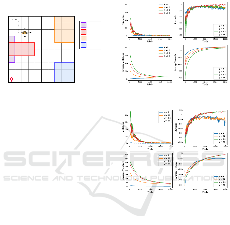
β
p
value set to 0.5. A diagram of the environment
with all constraints is shown in Fig. 3.
Cliff
Crime
Potholes
Storm
0.8
0.1
0.1
Figure 3: The taxi world environment with all constraints.
Figures 4 and 5 show the performance of the
ViGIS-P and ViGIS-L agents, respectively, in the 4-
constraint taxi world environment. As would be ex-
pected, the agents with higher β values generally
commit more violations. Interestingly, the β = 0.5
agents commit more violations early-on than the β =
0.8 agents. It is not clear what exactly causes this
behaviour, but it suggests that the choice of β should
be carefully tuned. The β = 0 agents are able to make
relatively few violations compared to the other agents,
but still does violate the safety constraints in spite of
β = 0 indicating zero tolerance of danger. Upon closer
investigation, it was found that all of these violations
occur at positions (1, 3) and (1, 6) on the grid: the
corner where the pit and crime constraints overlap. In
this case the agent’s safest actions are to move up-
wards or right, both of which incur a 10% probabil-
ity of violating a safety constraint. The agent is then
caught in a safe policy dead end, as described earlier.
The agents in Figures 4 and 5 are programmed to take
the action which corresponds to the highest reward
when in one of these dead ends, but other methods
are assessed in Figure 8. Comparing the violation and
reward rates, it is evident that the agents which com-
mit fewer violations also acquire fewer rewards. This
can be expected, because an agent would likely need
to take a sub-optimal path in order to avoid the con-
straints.
Figure 6 shows the performance of the ViGIS-P
and ViGIS-L agents compared to a regular RL agent.
Both ViGIS agents have their β values set to zero,
since this is the β value where both agents commit the
fewest violations. The ViGIS-P agent commits an av-
erage of 0.71 violations per trial, whereas the ViGIS-
L agent commits 0.20, which is ≈ 71% fewer viola-
tions. If we compare these agents to the β-pessimistic
Q-Learning agent, which makes ≈ 1.51 violations per
trial, the ViGIS algorithm makes ≈ 53% fewer viola-
Figure 4: The number of violations (left) and rewards (right)
per trial of ViGIS-P agent in the taxi world with all 4 con-
straints, and their respective running averages underneath.
Figure 5: The number of violations (left) and rewards (right)
per trial of ViGIS-L agent in the taxi world with all 4 con-
straints, and their respective running averages underneath.
tions, albeit at the cost of having a much less stable
reward curve. It is also worth noting that the regu-
lar Q-Learning agent vastly outperforms all three safe
algorithms in terms of rewards.
Figure 7 illustrates how both ViGIS algorithms
perform in the taxi world environment for all num-
bers of constraints. As would be expected, both
agents tend to violate the constraints more frequently
as more constraints are added. The number of vio-
lations committed by ViGIS-P increases significantly
when the number of constraints is increased from 1 to
2, but further increases only increase the number of
violations slightly. As was discussed earlier, all vio-
lations made by the ViGIS-P agent are in those two
safe policy dead end locations. Adding more con-
straints to the taxi world does not add any more dead
ends, but the state space that the agent explores be-
ICAART 2025 - 17th International Conference on Agents and Artificial Intelligence
282
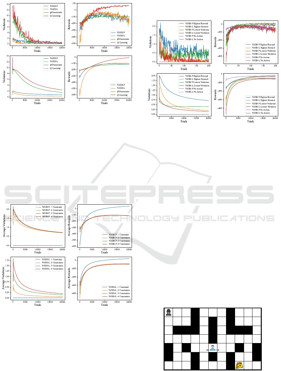
Figure 6: The number of violations (left) and rewards (right)
per trial of ViGIS-P and ViGIS-L compared to β-pessimistic
Q-Learning and regular Q-Learning. Results are from the
taxi world with all 4 constraints, and their respective run-
ning averages are beneath.
comes effectively smaller. This causes the agent to be
slightly more likely to commit enter these two dead
ends, which causes the slight further increase in vio-
lations when there are 3 or 4 constraints. On the other
hand, ViGIS-L shows an increase in violations that
is directly proportional to the number of constraints.
The ViGIS-L agent commits fewer violations than the
ViGIS-P agent for all constraint configurations.
Figure 7: A performance comparison between ViGIS-P
(top) and ViGIS-L (bottom) for different numbers of con-
straints. The average number of violations (left) and re-
wards (right) per trial in the taxi world are shown.
Figure 8 compares three different methods of han-
dling the safe policy dead end issue: choosing the ac-
tion with the highest expected reward, choosing the
action with the lowest expected violation, and choos-
ing no action. For both ViGIS agents, the lowest vi-
olation method performs causes fewer violations than
the highest reward method. The no action method is
able to avoid all violations, which shows promise for
this algorithm in safety-critical environments.
Figure 8: A comparison between different methods of han-
dling safe policy dead ends. The number of violations (left)
and rewards (right) per trial in the taxi world with all 4 con-
straints are shown, with their respective running averages
underneath.
5.2 Bank Robber
In this domain, the agent’s goal is to find the bank
vault, take the money, then return to the entrance -
avoiding the security guard as it does so. The agent’s
actions are completely deterministic but the security
guard patrols stochastically. After the agent chooses
a direction to move in, the security guard chooses a
random adjacent open square, with uniform proba-
bility, and moves to it. When the agent reaches the
exit with the money it receives a large reward, when it
takes the money it receives a small reward, and when
it is caught it receives a large penalty. Like in the taxi
world, the agent receives a default reward of −1 for
all other actions. Figure 9 shows an illustration of the
environment. The agents applied to this environment
are the same as for the taxi world environment. The
tolerance threshold for being caught and β are both
set to zero. The β-pessimistic agent has its β
p
value
set to 0.5.
Figure 9: The Bank Robber environment.
A Two-Phase Safe Reinforcement Learning Framework for Finding the Safe Policy Space
283
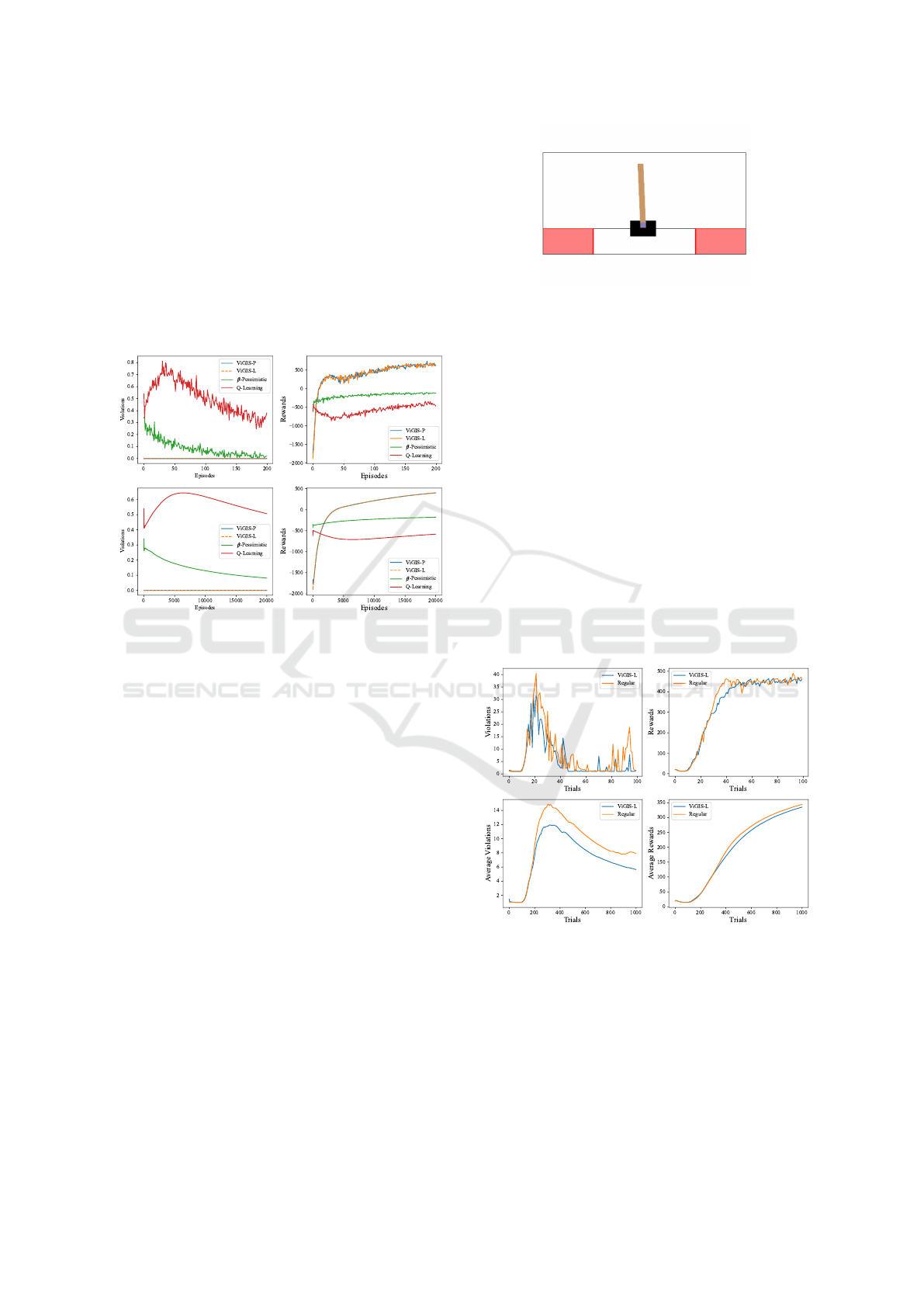
The performance of ViGIS in the bank robber en-
vironment compared to Q-Learning and β-pessimistic
Q-Learning is shown in Figure 10. Evidently, both
ViGIS-P and ViGIS-L make no violations at all, and
achieve a very high average reward by the end of
training. This shows the potential of ViGIS for envi-
ronments where the agent has complete deterministic
control over its own actions. ViGIS-P and ViGIS-L
produce almost identical reward curves, which shows
that both algorithms perform equally as well when
they find the same safe policy space.
Figure 10: The number of violations (left) and rewards
(right) per trial of ViGIS-P and ViGIS-L compared to β-
pessimistic Q-Learning and regular Q-Learning. Results are
from the bank robber environment with, and their respective
running averages are beneath.
5.3 Cart Pole
For the final problem domain, we make use of the
OpenAI Gym’s Cart Pole environment (Brockman
et al., 2016) with an added constraint: the agent’s po-
sition must remain between -0.5 and 0.5. In this envi-
ronment, the agent operates a cart with an attached
pole and must keep the pole upright by only mov-
ing the cart left or right. The agent receives a reward
at the end of each trial proportional to how long the
pole remained upright. At each step, the agent re-
ceives a reward of -1 if it is outside the bounds of
-0.5 and 0.5, otherwise it receives a reward of zero.
Figure 11 shows an illustration of the cart pole envi-
ronment. In this environment, we only test ViGIS-
L against a regular agent. Each agent uses a Dou-
ble Deep Q-Network (DDQN); ViGIS-L also uses a
DDQN to learn the safe policy space. These DDQNs
are comprised of 4 input neurons, 3 hidden layers with
128 neurons each, and 2 output neurons. The ViGIS-
L agent’s β value is set to zero: minimal tolerance for
violations.
Figure 11: The cart pole environment with the added con-
straint indicated in red.
Figure 12 shows the performance of a DDQN-
based ViGIS-L agent in the cart pole environment
compared to a regular DDQN agent. The violation
plot shows that after about 10 trials, both agents be-
gin to learn how to keep the pole up for long enough
to leave the boundaries specified by the constraints.
ViGIS-L commits significantly fewer violations than
the regular agent during this phase, which is more
clear from the running average. By the end of train-
ing, the regular agent has committed 7.92 violations
per trial on average, whereas the ViGIS-L agent has
committed 5.65. This shows a violation reduction of
more than 28%. Both agents achieve similar perfor-
mance reward-wise, however the regular agent does
outperform the ViGIS-L agent on average after about
350 trials. These results suggest that the ViGIS-L al-
gorithm was able to better avoid constraint violations,
albeit at a slight cost to performance. These results
show promise for ViGIS-L in deep RL.
Figure 12: The violations (left) and rewards (right) per trial
in the cart pole environment, as well as their respective run-
ning averages beneath.
6 CONCLUSION
This report presented a two-phase approach to safe
RL, ViGIS, which focuses on first finding the safe pol-
icy space, then performing RL within the safe policy
space. We described two implementations of ViGIS,
ICAART 2025 - 17th International Conference on Agents and Artificial Intelligence
284

named ViGIS-P and ViGIS-L. ViGIS-P requires prior
knowledge of the transition function but does not need
to simulate constraint violations, whereas ViGIS-L
needs violations to be performed in silico, but does
not require prior knowledge of the transition func-
tion. The fact that violations should be simulated for
ViGIS-L brings into question why we would not per-
form both phases in simulation. This is of course pos-
sible, but by separating the safety learning from re-
ward learning the agent is able to learn the reward
on-site, where the rewards would be more accurate.
Both ViGIS approaches were tested in two discrete
environments and ViGIS-L was also tested in a con-
tinuous environment.
Both ViGIS-P and ViGIS-L showed fewer con-
straint violations than the regular and β-pessimistic
Q-Learning agents across all environments. Often,
the better safety adherence lead the ViGIS agents to
achieve a lower average reward. ViGIS does en-
counter the problem of safe policy dead ends, but var-
ious methods of dealing with these dead ends were
assessed and it was found that choosing the safest
action significantly reduces the number of commit-
ted violations. It is also possible, in some environ-
ments and configurations, for ViGIS to avoid viola-
tions, which was shown for the bank robber environ-
ment and the taxi world environment for the No Ac-
tion ViGIS agents. ViGIS-L was able to make 28%
fewer constraint violations than the regular DDQN
agent in the cart pole environment, which shows its
potential in the realm of deep RL.
There are multiple avenues where the research in
this paper can be extended in future work:
• Scalability: investigate methods to optimize
ViGIS-P for larger state spaces, potentially
through approximation or parallelism.
• Deep RL: assess the performance of ViGIS with a
broader range of deep RL architectures.
• Normalising
ˆ
V
C
: develop analytical methods for
normalizing ViGIS-L’s violation measure.
• Hybrid Approaches: explore combinations of
ViGIS with other safe RL techniques to further
enhance safety and performance.
• Environments: Assess the performance of ViGIS
in more environments.
• Benchmarking: Compare ViGIS to additional
state-of-the-art safe RL algorithms.
REFERENCES
Altman, E. (1999). Constrained Markov Decision Pro-
cesses. Chapman and Hall.
Brockman, G., Cheung, V., Pettersson, L., Schneider, J.,
Schulman, J., Tang, J., and Zaremba, W. (2016). Ope-
nAI gym. arXiv preprint arXiv:1606.01540.
Driessens, K. and D
ˇ
zeroski, S. (2004). Integrating guid-
ance into relational reinforcement learning. Machine
Learning, 57:271–304.
Garc
´
ıa, J. and Fern
´
andez, F. (2012). Safe exploration of
state and action spaces in reinforcement learning. J.
Artif. Int. Res., 45(1):515–564.
Garc
´
ıa, J. and Fern
´
andez, F. (2015). A comprehensive sur-
vey on safe reinforcement learning. Journal of Ma-
chine Learning Research, 16(42):1437–1480.
Gaskett, C. (2003). Reinforcement learning under circum-
stances beyond its control.
Ge, Y., Zhu, F., Ling, X., and Liu, Q. (2019). Safe Q-
Learning method based on constrained Markov deci-
sion processes. IEEE Access, 7:165007–165017.
Geramifard, A., Redding, J., Roy, N., and How, J. (2011).
UAV cooperative control with stochastic risk models.
Kaelbling, L. P., Littman, M. L., and Moore, A. W. (1996).
Reinforcement learning: A survey. Journal of Artifi-
cial Intelligence Research, 4:237–285.
Mutti, M., Del Col, S., and Restelli, M. (2022). Reward-free
policy space compression for reinforcement learning.
In Camps-Valls, G., Ruiz, F. J. R., and Valera, I., ed-
itors, Proceedings of The 25th International Confer-
ence on Artificial Intelligence and Statistics, volume
151 of Proceedings of Machine Learning Research,
pages 3187–3203. PMLR.
Nana, H. P. Y. (2023). Reinforcement learning by minimiz-
ing constraint violation.
Russell, S. and Norvig, P. (2010). Artificial Intelligence: A
Modern Approach. Prentice Hall, 3rd edition.
Silver, D., Huang, A., Maddison, C. J., Guez, A., Sifre, L.,
van den Driessche, G., Schrittwieser, J., Antonoglou,
I., Panneershelvam, V., Lanctot, M., Dieleman, S.,
Grewe, D., Nham, J., Kalchbrenner, N., Sutskever, I.,
Lillicrap, T., Leach, M., Kavukcuoglu, K., Graepel,
T., and Hassabis, D. (2016). Mastering the game of
Go with deep neural networks and tree search. Na-
ture, 529(7587):484–489.
Srinivasan, K., Eysenbach, B., Ha, S., Tan, J., and Finn, C.
(2020). Learning to be safe: Deep RL with a safety
critic.
Thomas, G., Luo, Y., and Ma, T. (2024). Safe reinforcement
learning by imagining the near future. In Proceedings
of the 35th International Conference on Neural Infor-
mation Processing Systems, NIPS ’21, Red Hook, NY,
USA. Curran Associates Inc.
Xiong, N., Du, Y., and Huang, L. (2023). Provably safe
reinforcement learning with step-wise violation con-
straints. In Oh, A., Naumann, T., Globerson, A.,
Saenko, K., Hardt, M., and Levine, S., editors, Ad-
vances in Neural Information Processing Systems,
volume 36, pages 54341–54353. Curran Associates,
Inc.
Yang, W.-C., Marra, G., Rens, G., and De Raedt, L. (2023).
Safe reinforcement learning via probabilistic logic
shields. In Elkind, E., editor, Proceedings of the
Thirty-Second International Joint Conference on Arti-
ficial Intelligence, IJCAI-23, pages 5739–5749. Inter-
national Joint Conferences on Artificial Intelligence
Organization. Main Track.
A Two-Phase Safe Reinforcement Learning Framework for Finding the Safe Policy Space
285
