Revisit the Algorithm Selection Problem for TSP with Spatial
Information Enhanced Graph Neural Networks
Ya Song
a
, Laurens Bliek
b
and Yingqian Zhang
c
Eindhoven University of Technology, Eindhoven, Netherlands
Keywords:
Traveling Salesperson Problem, Algorithm Selection, Instance Hardness, Graph Neural Network, Graph
Classification.
Abstract:
Algorithm selection is a well-known problem where researchers investigate how to construct useful features
representing the problem instances and then apply feature-based machine learning models to predict the best
algorithm for each instance. However, even for simple optimization problems like Euclidean Traveling Sales-
man Problem (TSP), there lacks a general and effective feature representation for problem instances. The
important features of TSP are relatively well understood in the literature, based on extensive domain knowl-
edge and post-analysis of the solutions. In recent years, Convolutional Neural Network (CNN) has gained
popularity for TSP algorithm selection. Compared to traditional feature-based models, CNN has an automatic
feature-learning ability and demands less domain expertise. However, it is still required to generate interme-
diate representations, i.e., multiple images to represent TSP instances first. In this paper, we revisit algorithm
selection for TSP and propose GINES, a new Graph Neural Network (GNN) that uses city coordinates and
distances as input. GINES introduces a novel message-passing mechanism and local feature extractor to learn
TSP’s spatial information. Evaluation of two benchmarks shows GINES outperforms CNN and GINE mod-
els and surpasses traditional feature-based methods on one dataset. Our codes and datasets are available at
https://github.com/lurenyi233/GINES TSP.
1 INTRODUCTION
The Euclidean Traveling Salesman Problem (TSP) is
a widely studied NP-hard combinatorial optimization
problem with real-world applications and significant
theoretical value. It involves finding the shortest route
that visits a list of cities with known positions and re-
turns to the starting point. To solve this, researchers
have developed exact, heuristic, and learning-based
algorithms (Zhao et al., 2021b). Since algorithm per-
formance varies with problem instance characteris-
tics, selecting the right algorithm for each instance
can improve efficiency (Kerschke et al., 2018). Al-
gorithm selection for optimization problems is of-
ten treated as a classification task, where problem
instances are mapped to algorithms based on their
characteristics (Pereira et al., 2024). Typically, do-
main experts craft features (Bossek, 2017) to capture
TSP instance characteristics, which are then used to
train a machine learning classifier. However, This
a
https://orcid.org/0000-0001-6378-2212
b
https://orcid.org/0000-0002-3853-4708
c
https://orcid.org/0000-0002-5073-0787
feature-based method has several limitations: it re-
quires extensive domain knowledge, features may
lack expressiveness, and a feature selection process is
needed (Seiler et al., 2020). Handcrafted features do
not transfer well to other optimization problems, and
designing effective features for less-studied problems
than TSP is challenging.
Deep learning models, notably Convolutional
Neural Networks (CNN), are used to select TSP al-
gorithms by converting TSP instances into images,
making it a computer vision task. CNNs’ feature
learning eliminates the need for handcrafted fea-
tures. In (Seiler et al., 2020), a point image, a Mini-
mum Spanning Tree (MST) image, and a k-Nearest-
Neighbor-Graph (kNNG) image are generated for
each TSP instance, and an 8-layer CNN predicts the
best algorithm. In (Zhao et al., 2021b), TSP instances
are converted into density maps for classification us-
ing ResNet. A similar gridding method in (Huerta
et al., 2022) generates images to predict algorithm
performance over time with a 3-layer CNN.
Although CNNs outperform traditional models in
selecting algorithms for TSP (Huerta et al., 2022;
472
Song, Y., Bliek, L. and Zhang, Y.
Revisit the Algorithm Selection Problem for TSP with Spatial Information Enhanced Graph Neural Networks.
DOI: 10.5220/0013153400003890
Paper published under CC license (CC BY-NC-ND 4.0)
In Proceedings of the 17th International Conference on Agents and Artificial Intelligence (ICAART 2025) - Volume 3, pages 472-479
ISBN: 978-989-758-737-5; ISSN: 2184-433X
Proceedings Copyright © 2025 by SCITEPRESS – Science and Technology Publications, Lda.

Seiler et al., 2020; Zhao et al., 2021b), they have
notable drawbacks: (1) Need to generate intermedi-
ate representations. Like feature-based methods, gen-
erating image representations for CNN input is te-
dious. Generating MST and kNNG images involves
time-consuming calculations (Seiler et al., 2020), and
gridding with up-scaling is required for better resolu-
tion (Zhao et al., 2021b). Data augmentation like rota-
tion/flipping is widely used (Huerta et al., 2022), lead-
ing to the need for multiple images per instance. (2)
Introduce problem-irrelevant parameters. In (Seiler
et al., 2020), cities and connections in MST and
kNNG images are shown as solid dots and lines, but
these do not represent TSP properties. Setting image
size or grid number in gridding methods (Zhao et al.,
2021b) also adds complexity and needs extra param-
eter tuning. (3) Potentially lose problem-relevant in-
formation. The gridding process divides a TSP in-
stance into grids, with values denoting city counts.
This results in the loss of local structure. Addition-
ally, (Huerta et al., 2022) limits grid values, causing
further distortion. (4) Hard to generalize to other
routing problems. While gridding methods can turn
TSP instances into images due to their 2D nature,
they struggle with TSP variants like the Asymmet-
ric TSP (ATSP) and Vehicle Routing Problem (VRP).
Graphs with node/edge features may be more suitable
for these cases.
To address these issues, we introduce GINES, an
enhanced Graph Neural Network (GNN) for selecting
algorithms for TSP. Our key contributions are:
• We are the first to successfully design a GNN
to learn the representation of TSP instances for
algorithm selection, outperforming the existing
feature-based or CNN-based approaches.
• The proposed model merely takes the coordinates
of cities and the distance between them as inputs.
We show there is no need to design and generate
intermediate representations, such as handcrafted
features or images, for TSP instances.
• The adopted graph representation methodology
has few parameter settings, and the experimen-
tal results show it can retain accurate information
about the original TSP instances.
• The proposed model is able to capture local fea-
tures with multiple scales by aggregating infor-
mation from the neighborhood nodes. Its ro-
bust performance is demonstrated on two public
TSP datasets, compared with several existing ap-
proaches.
• The proposed model can easily generalize to other
complex routing problems by adding node fea-
tures or modifying distance metrics.
The paper is structured as follows: Section 2 cov-
ers background and related works, Section 3 presents
GINES, Section 4 details its experimental results, and
Section 5 concludes.
2 BACKGROUND AND RELATED
WORK
2.1 Algorithm Selection and Hardness
Prediction for Optimization
Problems
The No Free Lunch (NFL) theorem states that no
algorithm is universally optimal for all optimization
problems. Algorithm selection aims to improve over-
all solving performance by predicting the best al-
gorithm for each instance. Traditional approaches
rely on handcrafted features for specific problems
like TSP, VRP, and Knapsack Problem (Zhao et al.,
2021b). However, these features are often problem-
specific and require significant effort to design. Deep
learning models eliminate the need for tedious feature
engineering by automatically learning instance fea-
tures. For TSP, CNN-based models have been used
to generate intermediate representations such as im-
ages (Seiler et al., 2020; Zhao et al., 2021b). In
addition to the TSP, CNNs have also been utilized
for algorithm selection in various fields like Black-
Box Optimization (He and Yuen, 2020), commonly
by transforming instances into images or sequences.
However, graph-based representations remain under-
explored in this context.
Hardness prediction is a research topic closely
related to algorithm selection; it involves assessing
whether an instance is easy or difficult to solve us-
ing a specific algorithm (Jooken et al., 2022). Re-
searchers have identified attributes correlated with in-
stance hardness, such as clustering features, and edge
features (Mersmann et al., 2012). These features
are often used to evaluate TSP hardness for algo-
rithms like Ant Colony Optimization (ACO) and Lin-
Kernighan (LK) (Cris¸an et al., 2021). However, the
relevance of features can vary across algorithms, and
traditional feature-based machine learning models re-
main the primary approach in this field. To our knowl-
edge, deep learning models have not been explored
for hardness prediction.
2.2 Leveraging GNN for TSP
TSP instances can be effectively represented as
graphs, making GNNs a suitable tool for solving re-
Revisit the Algorithm Selection Problem for TSP with Spatial Information Enhanced Graph Neural Networks
473

lated problems. Current research on GNNs for TSP
focuses on three main areas:
GNN for TSP Solving. GNNs have been success-
fully applied in learning-based TSP solvers using re-
inforcement or supervised learning (Luo et al., 2023).
In reinforcement learning, models like Graph Pointer
Networks (Ma et al., 2019) is combined with Deep
Q-Learning to optimize policies. Supervised learn-
ing approaches often use GNNs as encoders, paired
with sequence-to-sequence architectures like Pointer
Networks (Vinyals et al., 2015). Hybrid models fur-
ther enhance efficiency by integrating GNNs with
heuristics. For example, Graph Convolutional Net-
work (GCN) predicts edge probabilities for optimal
tours (Joshi et al., 2019), while Graph Attention Net-
works (GAT) guide local search strategies (Hudson
et al., 2021). Recent work also highlights the impor-
tance of spatial distribution for improving generaliza-
tion (Jiang et al., 2022).
GNN for TSP Search Space Reduction. Search
space reduction transforms TSP into an edge classi-
fication problem, where GNNs predict edges likely
to be part of the optimal solution. For instance,
a kNNG represents TSP instances with node coor-
dinates and edge distances (Dwivedi et al., 2023).
This approach helps benchmark GNN architectures
for tasks like edge classification (Zhang et al., 2022)
and improves computational efficiency by narrowing
the search space.
GNN for TSP Algorithm Selection. Applying
GNNs for algorithm selection is still an emerging
field. Existing studies show CNNs outperform GCNs
for TSP algorithm selection due to GCN’s limita-
tions, such as the lack of node-level features and over-
smoothing (Zhao et al., 2021b). Current GNN re-
search in TSP solving and search space reduction of-
ten overlooks the spatial distribution of cities, which
is crucial for instance characterization. To address
this, we propose a tailored GNN architecture that in-
corporates spatial information to enhance algorithm
selection for TSP.
3 TSP ALGORITHM SELECTION
WITH GINES
3.1 Problem Statement
The TSP algorithm selection problem can be defined
as follows: given a TSP instance set I = {I
1
, I
2
, ..., I
l
},
a TSP algorithm set A = {A
1
, A
2
, ..., A
m
}, and a cer-
tain algorithm performance metric, the goal is to iden-
tify a per-instance mapping from I to A that maxi-
mizes its performance on I based on the given metric.
As discussed in previous sections, the TSP instances
can be represented by handcrafted features or images,
which are inputs to supervised learning models such
as SVM and CNN to learn this mapping.
In this work, we treat a TSP instance I
i
as a graph
G
i
= (V, E), where the node features X
v
for v ∈ V
is a vector of its (x
v
, y
v
) coordinate, the edge fea-
ture e
u,v
for (u, v) ∈ E is the Euclidean distance be-
tween two nodes. Here we use kNNG to represent
TSP instances. We set the number of nearest nodes
k to 10, which is relatively small compared to other
papers (Dwivedi et al., 2023) to reduce the compu-
tational burden. Let N be the number of cities. The
node feature is a [N, 2] matrix, and the matrix size of
the edge feature is [N × 10, 1]. Given a set of TSP
graphs {G
1
, G
2
, ..., G
l
} and their algorithm perfor-
mance labels {y
1
, y
2
, ..., y
l
}, the task of selecting TSP
algorithms can be converted to a graph-level classi-
fication task. We develop a GNN model for routing
problems, called GINES, which directly takes TSP
graphs as inputs for classification. Next, we will de-
scribe the architecture of this model in detail.
3.2 GINES
Graph Isomorphism Network (GIN) is one of the
most expressive GNN architectures for the graph-
level classification task. Researchers have shown
that the representational power of GIN is equal to
the power of the Weisfeiler Lehman graph isomor-
phism test, and GIN can obtain state-of-the-art per-
formance on several graph classification benchmark
datasets (Xu et al., 2018). GIN uses the following for-
mula for its neighborhood aggregation and message-
passing:
x
′
i
= MLP


(1 + ε) · x
i
+
∑
j∈N (i)
x
j


(1)
where x
i
is the target node’s features, N (i) denotes
the neighborhood for node i, and x
j
is the neighbor-
hood nodes’ features. ε indicates the significance of
the target node relative to its neighborhood, with a de-
fault value of zero. x
′
i
is the representation of node i
we get after applying one GIN layer. The function
MLP is a Multi-Layer Perceptron, which is used to
learn complex transformations of aggregated features.
Here, often the SUM aggregator is used to aggregate
information from the neighborhood, as it can better
distinguish different graph structures than MEAN and
ICAART 2025 - 17th International Conference on Agents and Artificial Intelligence
474

MAX aggregators (Xu et al., 2018). A drawback of
the original GIN is that the edge features are not taken
into account. Thus, the authors of (Hu et al., 2019)
proposed GINE that can incorporate edge features in
the aggregation procedure:
x
′
i
= MLP


(1 + ε) · x
i
+
∑
j∈N (i)
ReLU(x
j
+ e
j,i
)


(2)
where e
j,i
are edge features. In GINE, the neighbor-
hood nodes’ features and edge features are added to-
gether and make a ReLU transform before the SUM
aggregation. With a TSP graph, the dimensions of
these two features do not match. Therefore, we per-
form a linear transform to edge features.
To better tackle the TSP algorithm selection prob-
lem, we make several modifications on GINE and pro-
pose a GINES (GINE with Spatial information) archi-
tecture as follows.
Adopting a Suitable Aggregator. Aggregators in
GNNs play a crucial role in incorporating neighbor-
hood information and significantly impact represen-
tational capacity (Xu et al., 2018). Common aggre-
gators include MEAN, MAX, and SUM, each suited
for specific tasks. For instance, MEAN captures
node distribution and works well for distributional
tasks (Xu et al., 2018), while MAX highlights rep-
resentative nodes and is effective in vision tasks like
point cloud classification (Qi et al., 2017). SUM, used
by GIN, is ideal for learning structural graph proper-
ties. With post-analysis, researchers have shown that
the standard deviation (SD) or Coefficient of Varia-
tion (CV) of the distance matrix is one of the most
significant features (Cris¸an et al., 2021) in algorithm
selection or hardness prediction for TSP. Intuitively,
when the SD of the TSP distance matrix is very high,
it is easy to tell the difference between candidate so-
lutions, and the TSP is easy to solve. At the opposite
end of the spectrum, when the SD of the TSP distance
matrix is very small, there are many routes with the
same minimum cost, and finding one of them is not
difficult. So as the SD increases, an easy-hard-easy
transition can be observed. Based on the above anal-
ysis, we add the SD aggregator, along with the MAX
aggregator and SUM aggregator, as the three aggre-
gators in our GINES to aggregate useful information
for TSP algorithm selection.
Extracting Local Spatial Information. In a TSP
instance, cities are distributed in a 2D Euclidean
Space. The main characteristic to distinguish TSP
instances is the spatial distributions of cities. There
exists a research topic that also focuses on learning
the spatial distribution of points, namely, point cloud
classification. The point cloud is a type of practical
3D geometric data. Identifying point clouds is an ob-
ject recognition task with many real-world applica-
tions, such as remote sensing, autonomous driving,
and robotics (Qi et al., 2017). Unlike image data made
up of regular grids, the point cloud is unstructured
data as the distance between neighboring points is not
fixed. As a result, applying the classic convolutional
operations on point clouds is difficult. To tackle this,
researchers have designed several GNN architectures,
such as PointNet++ (Qi et al., 2017) and Point Trans-
former (Zhao et al., 2021a). In the message-passing
formulation of these GNNs for point clouds, a com-
mon component is (p
j
− p
i
), here p
i
and p
j
indicate
the positions of the current point and neighborhood
points, respectively. Through this calculation, local
neighborhood information, such as distance and an-
gles between points, can be extracted. As the TSP
instances can be viewed as 2D point clouds, extract-
ing more local spatial information may help identify
the TSP instances’ class. We add this component to
the message-passing formulation of GINES, as shown
follows:
x
′
i
=MLP (1 + ε) · x
i
+
M
j∈N (i)
ReLU

h
Θ
(x
j
− x
i
) + e
j,i

!
(3)
where
L
indicates the selected aggregator, it can be
either SD aggregator, MAX aggregator, or SUM ag-
gregator. h
Θ
is a neural network and defaults to be
one linear layer to transform the local spatial infor-
mation. The whole neural network architecture of our
GINES is shown in Figure 1. We adopt three GINES
layers to extract the salient spatial information from
TSP graphs and apply graph-level Sum pooling for
each GINES layer to obtain the entire graph’s repre-
sentation in all depths of the model. Then we con-
catenate these representations together and feed them
into the following two linear layers. We make full use
of the learned representation in the first two GINES
layers as they may have better feature generalization
ability (Xu et al., 2018).
4 EXPERIMENTS
4.1 Dataset
We evaluate the proposed GINES on two public TSP
algorithm selection datasets. The first dataset is gen-
Revisit the Algorithm Selection Problem for TSP with Spatial Information Enhanced Graph Neural Networks
475

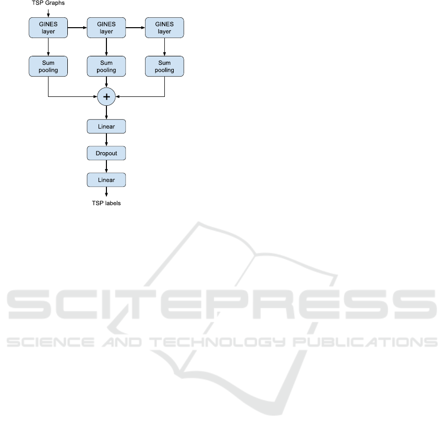
Figure 1: The GINES neural network architecture for TSP
algorithm selection.
erated to assess the Instance Space Analysis (ISA)
framework (Smith-Miles and van Hemert, 2011), and
the second is for evaluating the proposed CNN-based
selector (Seiler et al., 2020). The main difference be-
tween the two datasets is the size of the instances.
The TSP instances in the first dataset all contain 100
cities, while instances in the second dataset are rel-
atively larger and contain 1000 cities. Applying the
proposed model to two different datasets helps us ex-
amine its adaptability and compare it with other mod-
els. The following part is a detailed description of the
two datasets.
TSP-ISA Dataset. This dataset contains 1330
instances, each with 100 cities, divided into
seven groups based on characteristics: RAN-
DOM, CLKeasy, CLKhard, LKCCeasy, LKCChard,
easyCLK-hardLKCC, and hardCLK-easyLKCC. The
goal is to classify whether Chained Lin-Kernighan
(CLK) or Lin-Kernighan with Cluster Compensation
(LKCC) performs better. LKCC is the Single-Best-
Solver with an accuracy of 71.43% if applied to all
instances. To address class imbalance, random over-
sampling is used for training.
TSP-CNN Dataset. This dataset consists of 1000
instances, each with 1000 cities, and focuses on se-
lecting between two algorithms: Edge-Assembly-
Crossover (EAX) and Lin-Kernighan Heuristic
(LKH). The dataset is balanced, and EAX, as the
Single-Best-Solver, achieves 49% accuracy. In-
stances are specifically designed to favor one algo-
rithm over the other. A 10-fold cross-validation setup,
as used in (Seiler et al., 2020), ensures fair compar-
isons.
4.2 Baseline Model
To evaluate the performance of GINES, we com-
pare it with baseline models, which include traditional
feature-based methods and GNNs. For feature-based
models, we use Random Forest (RF) as the classi-
fier due to its effectiveness in TSP algorithm selec-
tion (Seiler et al., 2020). We evaluate four groups of
handcrafted TSP features:
• All140: All 140 TSP features defined by R pack-
age named salesperson (Bossek, 2017). These
features can be divided into 10 groups, including
Minimum Spanning Tree (MST) features, kNNG
features, Angle features, etc.
• Top15: after the feature selection procedure,
(Seiler et al., 2020) propose the best 15 TSP fea-
tures for the TSP-CNN dataset. Most of those
features are statistical values of strong connected
components of kNNG, and others are MST fea-
tures and Angle features.
• MST19: all the 19 MST features defined by
salesperson, are multiple statistical values of
MST distance and depth. Here we study the MST
features as MST is strongly related to TSP and
can be used to solve TSP approximately. Besides,
MST features are essential features for algorithm
selection according to the previous studies (Seiler
et al., 2020).
• kNNG51: all the 51 kNNG features defined by
salesperson, including statistical values of kNNG
distances, as well as the weak/strong connected
components of the kNNG.
For GNN baseline models, we include GCN and
GINE. Previous studies have shown that GCN per-
forms worse than CNN for TSP algorithm selec-
tion (Zhao et al., 2021b), while GINE offers stronger
representation learning capabilities and outperforms
GCN on graph-level tasks. This study is the first to ap-
ply GINE to algorithm selection. The baseline GNN
models share the same architecture and parameters
as GINES, except for replacing the three GINES lay-
ers with GCN or GINE. Additionally, we test GINES
with different aggregators: MAX (GINES-MAX),
SUM (GINES-SUM), and SD (GINES-SD). For con-
sistency, datasets are processed following (Seiler
et al., 2020), with 10-fold cross-validation on both the
TSP-ISA and TSP-CNN datasets. GNN models use
a hidden dimension of 32, and an Adam optimizer
with a learning rate of 0.01. Models are trained for
up to 100 epochs with early stopping (patience = 20).
ICAART 2025 - 17th International Conference on Agents and Artificial Intelligence
476

All experiments were conducted on a laptop with Intel
Core i7-9750H, and the code was implemented using
PyTorch Geometric.
4.3 Result and Analysis
Table 1 shows the average classification accuracy on
the TSP-ISA dataset, with the best and second-best re-
sults highlighted. Among feature-based approaches,
RF with all 140 features achieves the highest ac-
curacy, while using fewer features significantly re-
duces performance. MST features prove more ef-
fective than kNNG features in this task. GNNs out-
perform traditional feature-based models by automat-
ically extracting valuable features from kNNG. GINE
and GINES perform significantly better than GCN,
highlighting the importance of tailored GNN archi-
tectures for this application. By incorporating a spa-
tial information extractor, GINES achieves higher ac-
curacy than GINE. Tests with different aggregators
(MAX, SUM, SD) show comparable results, making
GINES a promising approach due to its high accu-
racy and independence from domain-specific feature
design.
Table 1: Algorithm selection performance comparison on
the TSP-ISA dataset.
Models Input data Accuracy
RF
All140 features 95.79 ± 2.26
Top15 features 87.37 ± 2.42
MST19 features 87.82 ± 2.73
kNNG51 features 74.36 ± 3.60
GCN kNNG 93.38 ± 1.71
GINE kNNG 97.52 ± 1.17
GINES-MAX kNNG 98.87 ± 0.91
GINES-SUM kNNG 98.87 ± 0.61
GINES-SD kNNG 98.42 ± 0.98
The experiment results on the TSP-CNN dataset
are shown in Table 2. Firstly, We apply the feature-
based models and find that RF with MST features
can achieve the best performance. Again, we can
observe that MST features are more valuable than
kNNG features in the TSP algorithm selection task.
Then we load the trained CNN model files and test
them to get CNNs’ performance. It shows that CNN
with Points+MST images is better than CNN with
other image inputs. At last, we test the proposed
GINES and baseline GNN models. GINES can out-
perform CNN models but is still worse than feature-
based models. The main reason may be the hand-
crafted features fed into RF are heavily engineered,
while the GNN models fail to extract some crucial
Table 2: Algorithm selection performance comparison on
the TSP-CNN dataset.
Models Input data Accuracy
RF
All140 features 73.30 ±5.10
Top15 features 73.40 ± 5.66
MST19 features 73.90 ± 4.81
kNNG51 features 72.80 ± 5.86
CNN
(Seiler et al., 2020)
Three images 70.50 ±7.55
Two images 72.00 ± 4.96
Points images 71.80 ± 6.63
GCN kNNG 62.80 ±5.86
GINE kNNG 66.30 ±3.93
GINES-MAX kNNG 70.20 ±5.19
GINES-SUM kNNG 70.00 ±4.47
GINES-SD kNNG 72.60 ±4.76
features, such as MST and clustering features. Be-
sides, there are much more nodes in this dataset,
leading to less salient spatial information that can be
learned. In GINES, selecting the SD aggregator for
message-passing is advantageous as it relates closely
to TSP problem hardness. Tests on GINES-MAX and
GINES-SUM confirm that using an SD aggregator
yields better predictions for the TSP-CNN dataset.
Table 3 summarizes the properties of the feature-
based model, CNN, and GINES on the TSP algo-
rithm selection task. Compared to deep learning mod-
els such as CNN and the proposed GINES, the tradi-
tional feature-based method suffers from the follow-
ing shortcomings. Firstly, substantial domain exper-
tise is required to design features. Secondly, as shown
in Figure 2, the important features of the TSP-ISA
dataset and the TSP-CNN dataset are significantly dif-
ferent, indicating that tedious feature engineering is
required to choose valuable features. Finally, these
selected features are probably inapplicable to other
routing problems. The experiment results in Table
2 show that the proposed GINES is a competitive
method, and it can slightly outperform CNN in pre-
diction accuracy. GINES has several other advan-
tages compared to CNN. Firstly, CNN takes multi-
ple images as inputs, i.e., Points image, MST image,
and kNNG image. Generating these images might
be burdensome work, and it is unclear which image
can better represent TSP instances. Contrary to CNN,
GINES directly takes cities’ coordinate and distance
matrices as inputs, and we do not need to prepare
intermediate representations like images. Secondly,
when generating images for CNN, several problem-
irrelevant parameters must be set, such as image size,
dot size, and line width in MST and kNNG images.
Tuning these parameters can be a heavy workload,
Revisit the Algorithm Selection Problem for TSP with Spatial Information Enhanced Graph Neural Networks
477

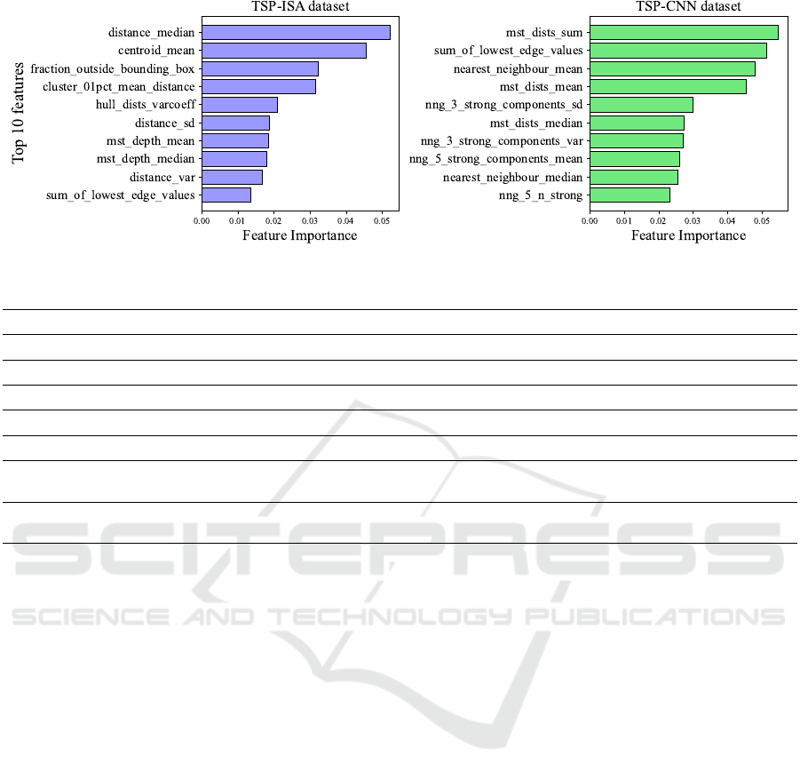
Figure 2: The Top 10 importance features for TSP-ISA dataset and TSP-CNN dataset.
Table 3: Properties comparison between Feature-based model, CNN, and GINES for algorithm selection.
Properties
Feature-based CNN (Seiler et al., 2020)
GINES
Intermediate representations Handcrafted features Points/MST/kNNG images
None
Feature Engineering
Yes No No
Problem-irrelevant parameters
None
Image size, Dot size, Line width
None
Data Augmentation
None
Random rotation/flipping
None
Problem-relevant information loss Domain dependent Resolution dependent
None
Generalize to VRP
(Distinguish different points)
Hard Hard
Easy to add
node features
Generalize to ATSP
(To Non-Euclidean Metric Space)
Hard Hard
Easy to add
edge features
although theoretically, these parameters should not
affect the learned mapping from instances to algo-
rithms. In GINES, on the other hand, the TSP in-
stances are treated as graphs, and there are not many
instance representation parameters to be designed or
adjusted. Besides, when setting the image resolution
in the CNN method, we should consider the city num-
ber in the TSP instance. Otherwise, the representation
ability of the image is inadequate, and problem in-
stance information is lost. At last, generating images
for TSP instances and applying CNN to select algo-
rithms is not very difficult because cities in TSP are
homogeneous and distributed in 2D Euclidean space.
If we look into some complex routing problems, we
will find that applying the CNN-based method is chal-
lenging. For VRP algorithm selection, it is hard to
differentiate the depot and customer with image rep-
resentations. While in GINES, we can simply add the
point features to tell them apart. Considering the rout-
ing problem in Non-Euclidean space such as ATSP,
drawing the problem instance on a 2D plane is nearly
impossible. While GINES can naturally recognize
the neighborhood in ATSP, we can also modify the
message-passing formulation in GINES to aggregate
more valuable edge features.
5 CONCLUSION
In this work, we propose a novel GNN named GINES
to select algorithms for TSP. By adopting a suit-
able aggregator and local neighborhood feature ex-
tractor, this model can learn useful spatial information
of TSP instances and outperform traditional feature-
based models and CNNs on public algorithm selec-
tion datasets. GINES handles TSP instances as graphs
and only takes cities’ coordinates and distances be-
tween them as inputs. Thus no intermediate represen-
tations for problem instances, such as features or im-
ages, need to be designed and generated before model
training. In contrast to converting TSP instances to
images, the graph representation is more natural and
efficient, as it neither introduces problem-irrelevant
parameters nor loses problem-relevant information.
The proposed GINES is promising as it is easy to
generalize to other routing problems. For example,
we can distinguish nodes and routes in the problem
instances by adding node features and edge features.
This work can be a good starting point for selecting
algorithms or predicting instance hardness for combi-
natorial optimization problems defined on graphs. In
the future, we will explore GINES architectures for
ICAART 2025 - 17th International Conference on Agents and Artificial Intelligence
478

more complex problems like ATSP, VRP, and real-
world problems.
REFERENCES
Bossek, J. (2017). Salesperson: computation of instance
features and r interface to the state-of-the-art exact and
inexact solvers for the traveling salesperson problem.
Cris¸an, G. C., Nechita, E., and Simian, D. (2021). On ran-
domness and structure in euclidean tsp instances: A
study with heuristic methods. IEEE Access, 9:5312–
5331.
Dwivedi, V. P., Joshi, C. K., Luu, A. T., Laurent, T., Bengio,
Y., and Bresson, X. (2023). Benchmarking graph neu-
ral networks. Journal of Machine Learning Research,
24(43):1–48.
He, Y. and Yuen, S. Y. (2020). Black box algorithm se-
lection by convolutional neural network. In Machine
Learning, Optimization, and Data Science: 6th Inter-
national Conference, LOD 2020, Siena, Italy, July 19–
23, 2020, Revised Selected Papers, Part II 6, pages
264–280. Springer.
Hu, W., Liu, B., Gomes, J., Zitnik, M., Liang, P.,
Pande, V., and Leskovec, J. (2019). Strategies for
pre-training graph neural networks. arXiv preprint
arXiv:1905.12265.
Hudson, B., Li, Q., Malencia, M., and Prorok, A.
(2021). Graph neural network guided local search
for the traveling salesperson problem. arXiv preprint
arXiv:2110.05291.
Huerta, I. I., Neira, D. A., Ortega, D. A., Varas, V., Godoy,
J., and As
´
ın-Ach
´
a, R. (2022). Improving the state-of-
the-art in the traveling salesman problem: an anytime
automatic algorithm selection. Expert Systems with
Applications, 187:115948.
Jiang, Y., Wu, Y., Cao, Z., and Zhang, J. (2022). Learning to
solve routing problems via distributionally robust op-
timization. In Proceedings of the AAAI Conference on
Artificial Intelligence, volume 36, pages 9786–9794.
Jooken, J., Leyman, P., and De Causmaecker, P. (2022). A
new class of hard problem instances for the 0–1 knap-
sack problem. European Journal of Operational Re-
search, 301(3):841–854.
Joshi, C. K., Laurent, T., and Bresson, X. (2019). An
efficient graph convolutional network technique for
the travelling salesman problem. arXiv preprint
arXiv:1906.01227.
Kerschke, P., Kotthoff, L., Bossek, J., Hoos, H. H., and
Trautmann, H. (2018). Leveraging tsp solver com-
plementarity through machine learning. Evolutionary
computation, 26(4):597–620.
Luo, F., Lin, X., Liu, F., Zhang, Q., and Wang, Z. (2023).
Neural combinatorial optimization with heavy de-
coder: Toward large scale generalization. Advances
in Neural Information Processing Systems, 36:8845–
8864.
Ma, Q., Ge, S., He, D., Thaker, D., and Drori, I. (2019).
Combinatorial optimization by graph pointer net-
works and hierarchical reinforcement learning. arXiv
preprint arXiv:1911.04936.
Mersmann, O., Bischl, B., Bossek, J., Trautmann, H., Wag-
ner, M., and Neumann, F. (2012). Local search and the
traveling salesman problem: A feature-based charac-
terization of problem hardness. In Learning and In-
telligent Optimization: 6th International Conference,
LION 6, Paris, France, January 16-20, 2012, Revised
Selected Papers, pages 115–129. Springer.
Pereira, J. L. J., Smith-Miles, K., Mu
˜
noz, M. A., and
Lorena, A. C. (2024). Optimal selection of bench-
marking datasets for unbiased machine learning algo-
rithm evaluation. Data Mining and Knowledge Dis-
covery, 38(2):461–500.
Qi, C. R., Yi, L., Su, H., and Guibas, L. J. (2017). Point-
net++: Deep hierarchical feature learning on point sets
in a metric space. Advances in neural information pro-
cessing systems, 30.
Seiler, M., Pohl, J., Bossek, J., Kerschke, P., and Traut-
mann, H. (2020). Deep learning as a competitive
feature-free approach for automated algorithm selec-
tion on the traveling salesperson problem. In Par-
allel Problem Solving from Nature–PPSN XVI: 16th
International Conference, PPSN 2020, Leiden, The
Netherlands, September 5-9, 2020, Proceedings, Part
I, pages 48–64. Springer.
Smith-Miles, K. and van Hemert, J. (2011). Discovering
the suitability of optimisation algorithms by learning
from evolved instances. Annals of Mathematics and
Artificial Intelligence, 61:87–104.
Vinyals, O., Fortunato, M., and Jaitly, N. (2015). Pointer
networks. Advances in neural information processing
systems, 28.
Xu, K., Hu, W., Leskovec, J., and Jegelka, S. (2018). How
powerful are graph neural networks? arXiv preprint
arXiv:1810.00826.
Zhang, H., Xu, M., Zhang, G., and Niwa, K. (2022). Ssfg:
Stochastically scaling features and gradients for reg-
ularizing graph convolutional networks. IEEE Trans-
actions on Neural Networks and Learning Systems.
Zhao, H., Jiang, L., Jia, J., Torr, P. H., and Koltun, V.
(2021a). Point transformer. In Proceedings of the
IEEE/CVF international conference on computer vi-
sion, pages 16259–16268.
Zhao, K., Liu, S., Yu, J. X., and Rong, Y. (2021b). To-
wards feature-free tsp solver selection: A deep learn-
ing approach. In 2021 International Joint Conference
on Neural Networks (IJCNN), pages 1–8. IEEE.
Revisit the Algorithm Selection Problem for TSP with Spatial Information Enhanced Graph Neural Networks
479