Impact of Biased Data Injection on Model Integrity in Federated

Learning

Manuel Lengl

1∗ a

, Marc Benesch

1∗ b

, Stefan R

ohrl

1 c

, Simon Schumann

1 d

, Martin Knopp

1,2 e

Oliver Hayden

2 f

and Klaus Diepold

1 g

Chair of Data Processing, Technical University of Munich, Germany

Heinz-Nixdorf Chair of Biomedical Electronics, Technical University of Munich, Germany

Keywords:

Federated Learning, Data Bias, Privacy Violation, Membership Inference Attack, Blood Cell Analysis,

Quantitative Phase Imaging, Microﬂuidics, Flow Cytometry.

Abstract:

Federated Learning (FL) has emerged as a promising solution in the medical domain to overcome challenges

related to data privacy and learning efﬁciency. However, its federated nature exposes it to privacy attacks and

model degradation risks posed by individual clients. The primary objective of this work is to analyze how

different data biases (introduced by a single client) inﬂuence the overall model’s performance in a Cross-Silo

FL environment and whether these biases can be exploited to extract information about other clients. We

demonstrate, using two datasets, that bias injection can signiﬁcantly affect model integrity, with the impact

varying considerably across different datasets. Furthermore, we show that minimal effort is sufﬁcient to infer

the number of training samples contributed by other clients. Our ﬁndings highlight the critical need for robust

data security mechanisms in FL, as even a single compromised client can pose serious risks to the entire

system.

1 INTRODUCTION

In recent years, Federated Learning (FL) has shown

promising results across various machine learning

ﬁelds, offering solutions to some key challenges. FL

successfully addresses critical issues such as insufﬁ-

cient training data, centralizing sensitive data, and low

training efﬁciency (Xu et al., 2022). However, every

type of collaborative training also introduces poten-

tial risks. As more parties become involved in the

training process, the likelihood of someone introduc-

ing ﬂawed data increases (Xu et al., 2022). While this

can occur unintentionally, for example, due to differ-

ing measurement setups, it can also be exploited in-

tentionally to disrupt the training process. Addition-

ally, Jegorova et al. (2022) showcase several scenarios

of privacy attacks against FL environments, demon-

strating their effects on data privacy.

https://orcid.org/0000-0001-8763-6201

https://orcid.org/0009-0005-6004-9644

https://orcid.org/0000-0001-6277-3816

https://orcid.org/0000-0002-7074-473X

https://orcid.org/0000-0002-1136-2950

https://orcid.org/0000-0002-2678-8663

https://orcid.org/0000-0003-0439-7511

These authors contributed equally to this work.

A ﬁeld where these concerns are particularly criti-

cal is the medical sector. The General Data Protection

Regulation (Voigt and von dem Bussche, 2017) in Eu-

rope imposes stringent requirements on patient data

privacy, making FL an attractive option for collabora-

tion between hospitals (Sohan and Basalamah, 2023).

However, any disturbances in the collaborative pre-

diction models are intolerable, as they could directly

impact patient safety. Therefore, it is crucial to inves-

tigate the potential risks posed by clients introducing

unintended or malicious changes to the training pro-

cess.

Quantitative Phase Imaging (QPI) is an emerging

technology in biology that generates complex image-

based data. It was already successfully applied in

several ﬁelds, including oncology (Lam et al., 2019)

and hematology (Fresacher et al., 2023; Klenk et al.,

2023). To harness its potential for solving medical

challenges with machine learning, it requires (like

many image classiﬁcation tasks) large datasets to de-

velop accurate classiﬁcation models. This depen-

dence on extensive data makes QPI an ideal use case

for exploring potential threats posed by injected bias,

which can severely affect model accuracy and relia-

bility.

This work aims to address key challenges in FL by

exploring two critical scenarios. First, we analyze the

432

Lengl, M., Benesch, M., Röhrl, S., Schumann, S., Knopp, M., Hayden, O. and Diepold, K.

Impact of Biased Data Injection on Model Integrity in Federated Learning.

DOI: 10.5220/0013153800003911

Paper published under CC license (CC BY-NC-ND 4.0)

In Proceedings of the 18th International Joint Conference on Biomedical Engineering Systems and Technologies (BIOSTEC 2025) - Volume 1, pages 432-443

ISBN: 978-989-758-731-3; ISSN: 2184-4305

impact of artiﬁcially inducing biases by one client to

intentionally degrade the model’s generalization ca-

pability and overall performance. The primary objec-

tive is to assess the extent to which injected biases

affect a model trained within a FL setup. Second,

we examine a speciﬁc white-box attack resembling

a Membership Inference Attack (Salem et al., 2019),

where the adversary seeks to reconstruct partial infor-

mation from other clients’ datasets, raising signiﬁcant

privacy concerns. In this scenario, we consider a ma-

licious actor with access to a single client’s data pool.

We analyze both scenarios on two distinct datasets

and explore whether systematically designing these

biases could successfully disturb the model and/or

extract insights into other clients’ data. Addition-

ally, we perform a statistical evaluation to determine

whether inherent dataset characteristics provide re-

silience against these attacks, i.e., whether one dataset

shows greater robustness compared to the other.

2 DATA

2.1 Image Acquisition

To show the impact of biased data on real-world ex-

amples, we used a Quantitative Phase Imaging (QPI)

setup to measure human blood samples.

2.1.1 Quantitative Phase Imaging

In general, microscopes based on QPI operate us-

ing the principle of interference between an object

beam and a reference beam to capture the phase shift

of light ∆φ. The shift provides information about

the optical density of the sample interrupting the

object beam. By combining QPI with a microﬂu-

idic channel and focusing system, this setup allows

for high-throughput sample measurement. Therefore,

this technology is particularly valuable for biomedi-

cal applications (Jo et al., 2019), as it addresses the

key challenge of traditional bright-ﬁeld microscopy.

In bright-ﬁeld microscopy, the transparent nature of

biological cells often results in low-contrast images,

making it necessary to apply molecular staining (Bar-

cia, 2007; Klenk et al., 2019). This staining step is

not only time-consuming but can also introduce addi-

tional errors in the processing pipeline. Phase imag-

ing, on the other hand, provides far more detailed in-

sights into cellular structures than intensity images,

without requiring prior labeling.

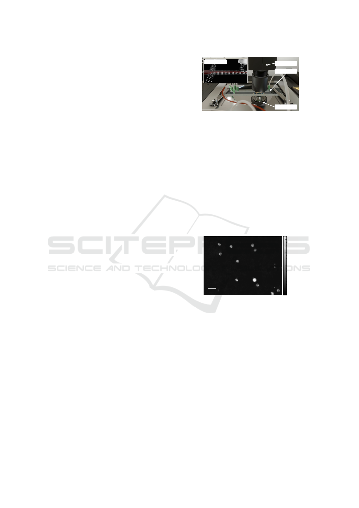
In this work, we used a customized differential

holographic microscope from Ovizio Imaging Sys-

tems, as illustrated in Figure 1. This system enables

Light Source

Fluidics Chip

Objective

Sheath Flows

Figure 1: Microscope setup.

label-free imaging of untreated blood cells in sus-

pension. Our approach is closely related to off-axis

diffraction phase microscopy (Dubois and Youras-

sowsky, 2008), but it uses a low-coherence light

source and does not require a reference beam. Cells

are precisely focused within a 50×500 µm polymethyl

methacrylate microﬂuidic channel. Four sheath ﬂows

are used to center the blood cells within the chan-

nel, preventing contact with the channel walls. This

setup allows for measuring 105 frames per second

with an average of 5 cells per frame. The resulting

frames have a size of 384×512 pixels, with an exam-

ple shown in Figure 2. Further details about this mi-

croscope are available in Dubois and Yourassowsky

(2011) and Ugele et al. (2018).

20 µm

∆φ in rad

Figure 2: Sample frame.

2.1.2 Pre-Processing

To prepare the image frames for further analysis, sev-

eral additional steps are necessary.

Background Cleaning. The output frames of the

microscope setup may contain background artifacts

and noise originating from the microﬂuidic channel or

camera lens. Due to the ﬁxed orientation of the lens,

camera, light, and microﬂuidics, these disturbances

tend to remain consistent during individual measure-

ments and, therefore, can be effectively approximated

by calculating the median of all images. By subtract-

ing this background approximation from each frame

individually, the resulting images are much cleaner

and ready for further processing.

Impact of Biased Data Injection on Model Integrity in Federated Learning

433

Segmentation. To identify individual cells in the

frames, we apply binary thresholding with a threshold

of 0.3 rad and extract patches with a size of 48 × 48

pixels around each detected cell. From these patches,

we extract binary masks that cover the areas of the in-

dividual cells. To further reﬁne the obtained masks,

we apply a Gaussian ﬁlter with a standard deviation

of σ = 0.5 (Gonzalez and Woods, 2002), smoothing

the mask transitions.

Filtering. Although the necessary biological pre-

processing steps are minimal, the high-throughput, to-

gether with the isolation process that is required to

isolate the different subtypes, can still result in the de-

struction of some cells. To ﬁlter out these damaged or

fragmented cells, we calculate the 2D area each cell

covers and discard any cell with an area smaller than

357 µm² (equivalent to 30 pixels). Cells or particles

below this threshold are typically remnants from the

isolation process.

2.2 Datasets

In this study, we use both a publicly available bench-

mark dataset and a curated, domain-speciﬁc dataset

from the medical ﬁeld to provide comprehensive in-

sights.

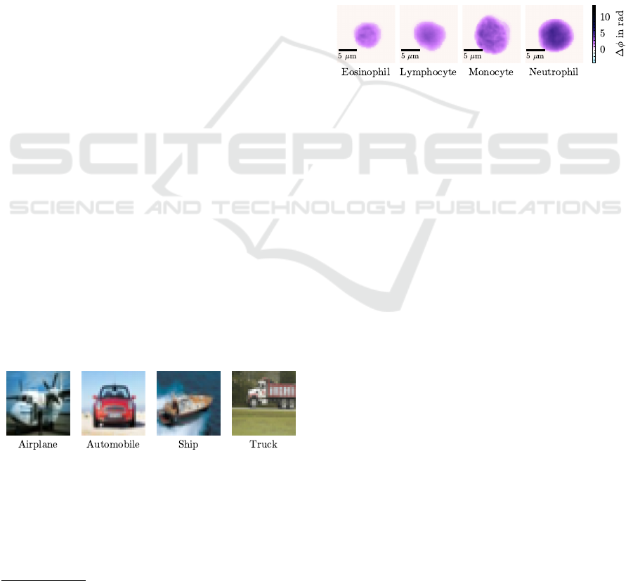
CIFAR-4. The ﬁrst dataset is derived from CIFAR-

10 (Krizhevsky, 2009), a well-known benchmark in

machine learning research, which we use as a refer-

ence for comparing results obtained from the Leuko-

cyte dataset. CIFAR-10 comprises 60,000 images,

each 32 × 32 pixels, evenly distributed across 10

classes. To facilitate a more realistic comparison, we

reduced this dataset to include only four classes —

airplane, automobile, ship, and truck — resulting in

the CIFAR-4 dataset, which aligns with the four-class

classiﬁcation structure of the Leukocyte dataset.

Figure 3: CIFAR-4 examples.

Leukocyte. The second dataset, acquired using our

setup described in Section 2.1, contains samples from

various leukocyte subtypes, with the goal of per-

forming a four-part differential

. This classiﬁcation

Basophils are excluded due to their low occurrence.

distinguishes between monocytes, lymphocytes, neu-

trophils, and eosinophils. We obtained the sepa-

rated cell types from whole blood samples by apply-

ing the isolation protocol according to Ugele (2019)

and Klenk et al. (2019). The complete dataset in-

cludes 447,541 images of white blood cells from

three healthy donors, each paired with a correspond-

ing segmentation mask. To align with our reference

dataset, CIFAR-4, which contains only 24,000 im-

ages, we reduced the Leukocyte dataset to the same

size. The sample distribution across the four classes

is balanced, and we applied a Min-Max scaling with

min = −1 and max = 7, normalizing the data to the

range [0, 1] (Bishop, 2006). It is important to note that

this dataset contains single-channel images, in con-

trast to the CIFAR-4 dataset with three-channel im-

ages.

Figure 4: Leukocyte examples. (Phase shift of the single-

channel images is color mapped to imitate the appearance

of a Giemsa stain (Barcia, 2007)).

3 METHODOLOGY

3.1 Classiﬁcation Model

For our experiments, we used a Convolutional Neu-

ral Network based on the AlexNet architecture

(Krizhevsky et al., 2017), which is well-established

in image classiﬁcation tasks. Our objective in this

work is not to further enhance the already high perfor-

mance of state-of-the-art models but rather to evaluate

the impact of data perturbations. Therefore, AlexNet

is an ideal choice for this purpose, as it offers strong

accuracy while maintaining a relatively low network

complexity, helping to minimize potential confound-

ing factors.

We retained the original AlexNet architecture,

only adapting the ﬁrst fully connected layer to accom-

modate the different numbers of input channels.

3.2 Federated Learning

As opposed to traditional machine learning, Feder-

ated Learning (FL) enables the cooperation of several

clients to train a common model; without needing to

exchange, share, and store data centrally (McMahan

et al., 2017). Instead of sharing data, the participat-

BIOINFORMATICS 2025 - 16th International Conference on Bioinformatics Models, Methods and Algorithms

434

ing clients exchange only weight updates from their

locally trained models. In this work, we focus on a

setup with an aggregation server that serves as a cen-

tral orchestrating entity. The server updates its global

model by applying the exchanged weight updates and

returns them to the clients. Each cycle of this process

can be described as one training round.

The overall FL setting can be categorized based

on the topology and data partitioning (Rieke, 2020).

A Cross-Device topology is characterized by a scal-

able and often large number of clients, which may not

always be available. In contrast, a Cross-Silo topol-

ogy involves a smaller number of clients that typi-

cally have identical setups and are always reachable

(Kholod et al., 2020). Data partitioning is typically

classiﬁed into two primary types. In horizontal par-

titioning, each client holds a different subset of data

that shares the same features. Converseley, in vertical

data partitioning, the data is split based on features

rather than samples.

In this work, we focused on a horizontal Cross-

Silo setup, which ﬁts well with our clinical context

and imaging data. For this setting, we can describe

the problem of training a machine learning model in

a federated manner as minimizing the objective func-

tion

f(w

,..., w

) =

∑

k=1

), w

∈ R

, (1)

where K is the number of clients and f

) is the

local objective function of one client with model

weights w

corresponding to that speciﬁc client’s

dataset. We assume a theoretical dataset D =

{(x

),..., (x

)} with N being the total num-

ber of samples, partitioned across the K clients.

The dataset is partitioned such that D =

and

= {}, hence each client holds n

= |D

| sam-

ples. The local optimization problem can be formu-

lated as

min

ℓ(x,y;w

) = min

∑

i∈D

ℓ(x

), (2)

where ℓ(·) is some loss function.

For the aggregation of the weights on the cen-

tral server, we use the Federated Average approach

ing session starts with the central server distributing

a random set of initial weights w

(t)

(with t = 0) to

the clients. Note that w

(t)

denotes the global model

weights, while w

(t)

represents the local model weights

for client k. A local update is then performed using,

for example, gradient descent

(t+1)

← w

(t)

− η∇ℓ(·;w

(t)

), (3)

where η is the learning rate.

The server aggregates the updated local weights

using a weighted average to compute the global model

for the next time step

(t+1)

← w

(t)

− η

∑

k=1

∇ℓ(·;w

(t)

), (4)

where

∑

k=1

∇ℓ(·;w

(t)

) = ∇ℓ(·;w

(t)

). Multiple local

updates using Equation 3 can be performed before the

central aggregation continues with the next time step

t + 1 (McMahan et al., 2017).

In our experiments, we used an independent and

identically distributed data split to avoid additional

complexity or noise. Our implementation is based on

the Flower

Python framework, designed for simulat-

ing FL procedures.

3.3 Bias Types

To investigate the impact of a single client contribut-

ing biased images, we applied various types of biases.

Each bias has a variable that controls the severity of

the bias, we later refer to this as bias strength. Note

that if the application of a bias results in pixel values

outside the normalized range [0,1], these values are

clipped.

Brightness. The brightness of an image refers to the

overall lightness or luminance of the image. It is a

perceptional term that describes how light or dark an

image appears to a viewer. Brightness is generally

associated with the intensity of light that the viewer

perceives from the image (Gianfrancesco et al., 2018).

Technically, brightness in an image can be quantiﬁed

by the average intensity of the pixels in the image.

Each pixel has a brightness value, which is typically

represented on a scale from 0 to 255 for all three

color channels, where 0 represents black (no bright-

ness) and 255 represents white (full brightness). By

adding a constant value to the pixel values, one can

artiﬁcially let the image be perceived as brighter or

darker. In this work we added different values in the

range of [−1,1] to achieve this.

Contrast. Contrast refers to the spread of the pixel

intensities of an image. High contrast images dis-

play a large difference between light and dark areas,

whereas low contrast images might appear ﬂat or dull

due to the closer range of tones. Contrast manipula-

tion is a common technique extensively described by

Gonzalez and Woods (2002). In 8-bit images normal-

ized to pixel values in the range [0, 1], we can deﬁne

https://ﬂower.ai/

Impact of Biased Data Injection on Model Integrity in Federated Learning

435

a neutral value, called midpoint in our implementa-

tion, around which contrast adjustments are centered.

Given the pixel range of the images, this value is typ-

ically 0.5. We can manipulate the contrast by scaling

the difference from the midpoint by a contrast fac-

tor α, and then adding the midpoint back to the pixel

value.

new

= α· (X

old

− 0.5) + 0.5. (5)

The transformation in Equation 5 scales the pixel val-

ues of image X

old

around the midpoint based on the

contrast factor α, where the operations are applied

element-wise.

Gaussian. Adding Gaussian noise to a clear im-

age can be viewed as simulating real-world condi-

tions for testing image processing algorithms since

almost no imaging technology is free of noise (Gon-

zalez and Woods, 2002). Using it as artiﬁcial and sys-

tematic bias requires drawing from the same distribu-

tion z ∼ N(µ,σ

), but varying a parameter ε such that

a pixel value x

i, j

is transformed as

new,i, j

= x

old,i, j

+ ε· z. (6)

We used Equation 6 with z ∼ N(0,1) in our imple-

mentation.

Edge. Convolving an image with special kernel ma-

trices ω

ω, which are well-known from image process-

ing, apply some effect to the image depending on the

kernel. This can be used to amplify or decrease the

extracted features from the original image X. A gen-

eral approach can be mathematically formulated as

new

= X

old

+ b· M, (7)

where M is a binary mask to identify the entries of the

matrix that are greater than a threshold T

M = ω

ω∗ X

old

> T =

(

0, x

i j

≤ T

1, x

i j

> T

. (8)

The entries of M are ampliﬁed by a scalar bias value

b, which can be negative or positive. For the sake

of simplicity, Equations 7 and 8 take only gray-scale

images into consideration. But the same can be ap-

plied to multi-channel images, too. We mainly used

an edge-detection kernel with

ω =





−1 −1 −1

−1 8 −1

−1 −1 −1





(9)

to emphasize the edges within the image, enhancing

their visibility.

Box Blur. We can introduce a Box Blur bias to sim-

ulate the effect of some imperfections by smoothing

out the image details (Gonzalez and Woods, 2002),

which mimics the loss of ﬁne detail often seen in real-

world data acquisition. One can also use this to build

a more robust model with higher generalization ca-

pability. We will examine this effect to see to what

extent this type of bias leads to more robustness and

when it results in performance degradation.

Similar to the edge detection, we convolve an im-

age with a kernel ω

ω:

ω =





1 1 1





, (10)

which averages a pixel value based on the neighbor-

ing pixels. The size of the kernel determines the blur

effect. We stick to one blur effect, but instead adjust

the strength of it by using Alpha Blending (Hughes,

2014). Essentially, we interpolate between the origi-

nal image and the blurred image to control how much

of the blurred image is mixed with the original image

based on the parameter ρ. Mathematically, we per-

form the following transforming steps:

filtered

= ω

ω∗ X

old

, (11)

new

= (1 − ρ) · X

old

+ ρ· X

filtered

. (12)

Adversarial. Adversarial attacks involve intention-

ally adding malicious perturbations to a model’s input

to deceive it. While there are different types of attacks

(Alhajjar et al., 2021), this work focuses on extraction

attacks in a white-box scenario, as they align with our

second goal of gaining knowledge from other clients.

Before diving further into the details of our approach,

we will provide a linear explanation of why adversar-

ial examples are effective.

Due to limited input feature precision and quanti-

zation in digital images, for instance, a pixel intensity

below the threshold of

255

(for 8-bit representation,

= 256) cannot be captured and is effectively dis-

carded. If we add a perturbation z smaller than the

feature precision to the original signal x, we obtain

x = x + z. A model will not be able to distinguish be-

tween x and

x, as long as the perturbation is bounded

by {z :∥ z ∥

∞

= max

| ≤ ε}. Now, consider a ma-

chine learning model with a weight vector w. Ap-

plying this weight vector to the adversarial example

gives:

⊤

x = w

⊤

x + w

⊤

z. (13)

This implies two things. First, w

⊤

z inﬂuences the

activation. Second, since ∥ z ∥

∞

is independent of

the dimension of z, but w

⊤

z increases (or decreases)

BIOINFORMATICS 2025 - 16th International Conference on Bioinformatics Models, Methods and Algorithms

436

with the dimension of w, this causes a compound ef-

fect, leading to a signiﬁcant change in the output for

high dimensional spaces (which is particularly rele-

vant for deep learning models). We can amplify this

effect by selecting z = sign(w) while ensuring the

constraint on z holds. Note that this does not mean

z exceeds the ε-bound; instead, we choose ε such that

∥ ε · sign(w) ∥

∞

= ε (Madry et al., 2017). Also, note

that the sign function is applied element-wise (Good-

fellow et al., 2014).

Goodfellow et al. (2014) introduced a computa-

tionally efﬁcient technique to approximate these per-

turbations: the Fast Gradient Sign Method (FGSM).

This method assumes a loss function ℓ(w,x, y), where

w are the parameters of a neural network. We can then

obtain an optimal max-norm constrained perturbation

(Goodfellow et al., 2014)

z = ε· sign(∇

ℓ(w,x, y)). (14)

Varying ε controls the magnitude of the perturba-

tion added to the image, and its optimal value ranges

heavily depend on the dataset and domain.

3.4 Inverse Problem Solving

For the goal of inferring information about the

datasets of other clients, we formulate the challenge

as an inverse problem since the malicious client does

not have direct access to the sample counts of other

clients. Mathematically, we assume a ﬁxed dataset

D, where subsets of this dataset represent the data

shares of different clients in a FL framework. D

de-

notes the dataset of a compromised client, whereas

represent the dataset of all other clients, such that

D = D

∪ D

and D

= D \D

. Our goal is to esti-

mate |D

|, when only D

is known. We have access

to the results of a forward map f (D

), which we

observe as

y = f (D

) + z, (15)

where y are vectors of metrics from FL training pro-

cesses for all biases and z represents uncertainty in the

forward model, accounting for ﬂuctuations observed

during training. These ﬂuctuations arise from the ran-

domness introduced during bias injection and train-

ing

, even with a ﬁxed seed.

Consequently, we employed three different super-

vised machine learning models - Linear Regression

(LR) (James et al., 2013), Support Vector Regression

(SVR) (Vapnik et al., 1996), and Random Forest Re-

gression (RFR) (Breiman, 2001) - as inverse problem

solvers to estimate the number of traning samples the

for example due to mini-batch sampling differences and stochastic op-

timization techniques

other clients have contributed D

. Figure 5 provides

a visualization of this approach.

Figure 5: Overview of the pipeline setup for solving the

inverse problem.

For simplicity, we assume that the total number of

training examples across all clients remains constant.

A more complex version of this problem could be for-

mulated without this assumption.

We conduct multiple simulations with varying ra-

tios between D

and D

. In each simulation, we apply

the biases described in Section 3.3 and perform sev-

eral FL trainings. The resulting metric vector is saved

as one observation for each ratio, respectively. This

process is summarized in the following algorithm:

Algorithm 1: Dataset Size Variation Analysis in Federated

Learning with Bias Injection.

1: Fix dataset D

2: for each ratio in set of ratios do

3: Split dataset D into D

and D

4: for each bias in grid do

5: Apply bias to D

6: Perform FL training with D

and D

7: Calculate metrics as observation y

8: end for

9: end for

After analyzing the loadings of a Principal Com-

ponent Analysis (Bishop, 2006) performed on the ob-

servations, we discard features with redundant infor-

mation. The input to the regression models then in-

clude Bias Type, Strength, Kullback-Leibler Diver-

gence, and Accuracy. Exemplary samples are shown

in Table 1.

Table 1: Exemplary inputs for the regression models.

Bias Type Strength KL-D Accuracy

Gaussian 0.05 0.02 0.95

Edge 0.4 0.07 0.88

...

Impact of Biased Data Injection on Model Integrity in Federated Learning

437

3.5 Evaluation Metrics

For evaluating the performance of the classiﬁcation,

we calculate Accuracy as a general performance met-

ric and the F1 score to have a balanced metric be-

tween false positives and false negatives (Bishop,

2006). Additionally, we calculate the Kullback-

Leibler Divergence (KL-D) to quantify how the distri-

bution of the predictions of the biased models deviates

from that of the unbiased model (Bishop, 2006). KL-

D is particularly sensitive to small changes, making it

useful for capturing subtle effects of bias variations.

However, it assumes a probability distribution, so it is

necessary to normalize the prediction frequencies by

the total number of predictions. This process is illus-

trated in Figure 6.

Figure 6: Using KL-D in a four-class classiﬁcation task.

The evaluation of the inverse problem solver

is performed using the Root Mean Squared Error

(RMSE) between the predicted and the actual dataset

size.

3.6 Training Setup

For training AlexNet, we use the Adam optimizer

with a ﬁxed learning rate of 0.001. The model is

trained with a batch size of 32, and we use Cross En-

tropy as the loss function (Goodfellow et al., 2016).

Training is conducted over 4 FL rounds with 3 epochs

each, and 4 participating clients. For the RFR we use

100 trees with a maximum depth of 10. The minimum

number of samples per leaf is set to 2, and the mini-

mum number of samples required to split an internal

node is 5. The SVR is implemented using the radial

basis function kernel, a regularization parameter of 1

and an ε value of 0.1. These parameters were experi-

mentally determined after performing a grid search.

All experiments are run for 5 different random

seeds. For the AlexNet, we always use 4,000 sam-

ples as test set, and the remaining ones are split into

training and validation with a ratio of 75:25.

4 RESULTS

4.1 Bias Injection Impact on Federated

Learning Performance

In the ﬁrst experiment, we analyze the impact of a sin-

gle client applying various bias types and strengths to

their share of data on the performance of our two dis-

tinct datasets. Even with identical training procedures

and bias strengths, the impact is expected to vary sig-

niﬁcantly depending on the dataset.

4.1.1 Results on Single Dataset

Initially, we visually assess how different strengths of

biases affect the model performances. For easier vi-

sual comparability, we normalized the bias strengths

to either [−1,1] or [0, 1], depending on the possible

signs of their strength variable. For the analysis, we

focus on Accuracy as the primary performance met-

ric, but the tendencies remain the same across all met-

rics. The resulting curves are expected to show a re-

versed U-shape or V-shape for biases that can have

both positive and negative strengths, indicating that

with stronger absolute bias, performance decreases.

For biases with only positive strengths, the curve will

show a one-sided shape.

To then statistically evaluate the signiﬁcance of

these effects, we apply a One-Sample t-Test

(James

et al., 2013), which compares the mean performance

under a certain bias with a hypothetical mean (i.e., the

performance without bias). Since we ran our simula-

tions with different random seeds, we can calculate

the mean and variance of a speciﬁc metric (e.g., Ac-

curacy) for each bias and strength. The hypotheses

for the t-Test are formulated as follows:

• Null Hypotheses (H

): There is no signiﬁcant dif-

ference in performance when a speciﬁc bias and

strength is applied.

We assume normal distribution due to various sources

of randomness during training (e.g., weight initialization,

optimization, data shufﬂing). Each model prediction can be

considered a random variable, and according to the Central

Limit Theorem (Moore et al., 2017), the sum or average of

many such random variables tends to follow a normal dis-

tribution. A Shapiro-Wilk test (Moore et al., 2017) further

supports this assumption, although it has lower power for

small sample sizes.

BIOINFORMATICS 2025 - 16th International Conference on Bioinformatics Models, Methods and Algorithms

438

• Alternative Hypotheses (H

): The change in per-

formance due to the speciﬁc bias and strength is

signiﬁcant.

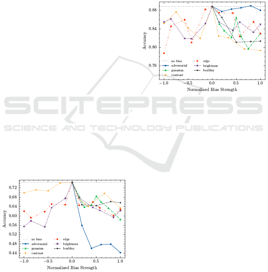
CIFAR-4. For the CIFAR-4 dataset, Figure 7 shows

the Accuracy across different bias types as a function

of bias strength. The corresponding p-values are pre-

sented in Table 5.

Starting with Brightness and Edge biases, the

curves exhibit the expected inverse U-shape. Low

bias has minimal effect on the model’s performances

across all metrics. However, as the absolute bias

strength increases, performance drops signiﬁcantly,

which is supported by the statistical test showing sig-

niﬁcant impact for almost all strength levels. Inter-

estingly, for Brightness, there is a slight skew notice-

able: negative strength values cause a larger decline

than equivalent positive values, a result that is further

conﬁrmed by the t-Test.

The effect of Contrast bias diverges from expec-

tations. While positive strength results in the ex-

pected performance decreases, negative values do not

show this tendency. They appear to have little in-

ﬂuence, with performance decreasing only slightly

with stronger negative values. Consequently, negative

strengths do not show a signiﬁcant impact.

Gaussian noise almost consistently degrades per-

formance as strength increases, with a counter-

intuitive outlier for a normalized strength of 0.5. This

anomaly is likely due to experimental errors.

The Box Blur bias shows a steep initial decrease

in performance, which then quickly saturates. Even

at maximum blur (normalized bias strength = 1.0), the

performance drop remains mostly unchanged. Addi-

tionally, this bias has high standard deviations, mak-

ing it difﬁcult to draw deﬁnitive conclusions about its

impact.

Figure 7: Accuracy across different bias types and strengths

for the CIFAR-4 dataset. All data points show the mean of

5 runs, standard deviation is not shown for clarity.

Finally, following the theoretical explanation in

Section 3.3, we successfully create Adversarial at-

tacks that highly impact the model’s performance.

Even with small perturbations (e.g., normalized

strength = 0.2), imperceptible to the human eye, the

metrics show a substantial drop with high conﬁdence

(i.e., low standard deviation). Max-norm perturba-

tions above 0.4 induced by the FGSM algorithm dras-

tically reduce Accuracy to between 0.4 and 0.5, which

is quite poor for a four-class classiﬁcation task. These

ﬁndings are further supported by very low p-values.

Figure 8: Accuracy across different bias types and strengths

for the Leukocyte dataset. All data points show the mean of

5 runs, standard deviation is not shown for clarity.

Leukocyte. In the Leukocyte dataset, as shown in

Figure 8, the effects of biases are generally less pro-

nounced, which is supported by the higher p-values in

Table 5 in the appendix.

For Brightness and Edge bias, the decline in per-

formance is minimal. However, a subtle U-shape is

apparent, suggesting that higher bias values have a

slightly greater impact on the model than lower ones.

Brightness shows again a slight skewness, both visu-

ally and statistically, but overall, the impact remains

surprisingly low (especially given that this bias could

alter the apparent size of the cells).

The behavior of Contrast shows again a skewed

U-shape, with a tendency for less impact when Con-

trast is decreased. However, the effect of negative

strengths is more noticeable than in the CIFAR-4

dataset. Overall, no bias strength yields a signiﬁcant

impact.

For Gaussian noise, we observe a gradually in-

creasing decline in performance. While the impact is

not drastic, each noise level still results in a measur-

able performance drop. The curve looks quite similar

to the pattern seen for CIFAR-4, with a similar peak at

0.5, making it worthwile to investigate further.

With Box Blur, added to the cell images, the

Impact of Biased Data Injection on Model Integrity in Federated Learning

439

model’s performance degrades, but the impact satu-

rates once the normalized strength exceeds 0.5. Fur-

ther increases do not cause any noticeable changes in

performance drop. All impacts are again statistically

signiﬁcant.

Adversarial attacks show a much smaller effect

than anticipated. While we would expect stronger

adversarial perturbations to severely degrade the

model’s performance, the actual impact is minimal.

The model’s Accuracy remains largely unaffected

across the range of adversarial strengths, indicating

that the dataset is relatively robust to these attacks.

4.1.2 Comparison

The p-values in Table 5 together with the visual in-

spection in the previous sections already suggest that

the CIFAR-4 dataset is generally more sensitive to the

introduced biases compared to the Leukocyte dataset.

To statistically evaluate whether one dataset is inher-

ently more robust against different types of biases, we

conducted a two-way ANOVA (Moore et al., 2017),

assessing the effect of the dataset. This allows us

to test whether the differences in robustness between

the two datasets are statistically signiﬁcant. While

ANOVA traditionally compares group means, we for-

mulate hypotheses to interpret whether one dataset is

signiﬁcantly more robust to the biases than the other:

• Null Hypothesis (H

): There is no signiﬁcant

difference in robustness between Leukocyte and

CIFAR-4 when a speciﬁc bias is applied, imply-

ing similar performance changes.

• Alternative Hypothesis 1 (H

): There is a signif-

icant difference in robustness between Leukocyte

and CIFAR-4 when a speciﬁc bias is applied, im-

plying that performance for one dataset is signiﬁ-

cantly more impacted.

The null hypotheses H

can be rejected for a given

bias type if the p-value is below 0.05.

Table 2 summarizes the outcome of the analysis.

The results show, that for several bias types, there is

a signiﬁcant difference in robustness. Four out of six

types have a p-value below 0.05, with extremely low

values in some cases. Conﬁrming with Table 5 to see

which dataset is impacted more heavily shows that the

Leukocyte dataset is more robust in all four cases of

Adversarial, Brightness, Edge, and Gaussian Bias, al-

though the signiﬁcance for the latter is not as strong

as for the others.

For the Box Blur, both datasets are impacted sig-

niﬁcantly, with no inherent difference, even though

the p-value is relatively small at p = 0.076. Interest-

ingly, in the case of the Contrast bias, there is no dif-

ference at all, suggesting that both datasets are simi-

larly affected (or not affected) by changes in strength.

Table 2: Results of a two-way ANOVA to assess whether

one dataset is inherently more robust against different bias

types. p-values below 0.05 are marked in bold.

Bias Type df(D,R) F-value p-value

Adversarial (1,48) 218.53 1.71 × 10

−19

Box Blur (1,38) 3.33 0.07601

Brightness (1,97) 63.95 2.72 × 10

−12

Contrast (1,78) 0.13 0.72458

Edge (1,97) 31.73 1.73 × 10

−7

Gaussian (1,67) 10.49 0.00187

4.2 Systematic Knowledge Extraction

from Other Clients

In the second experiment, we aim to infer informa-

tion about the datasets of other clients. As an initial

approach, we attempt to estimate the ratio of data con-

tributed by each client - speciﬁcally, how many sam-

ples other clients contribute to the training process.

We vary the ratio by adjusting the number of samples

contributed by the compromised client. As input for

the prediction, we use the observations of the metrics

y derived from various FL training runs under differ-

ent ratios and induced biases.

4.2.1 Results on Single Dataset

We ﬁrst evaluate the success of the attack on individ-

ual datasets. For this purpose, we train regression

models to predict the amount of training data con-

tributed by the other client. Additionally, to support

the general assumption of a correlation between the

malicious clients’ share of data and the resulting drop

in performance, we visually examine whether a trend

is present.

CIFAR-4. Table 3 presents the outcomes for the

three regression models. When considering all bias

types and strengths, RFR performs best with a RMSE

of 3,812. Given that the maximum number of train-

ing samples is 20,000 images, a RMSE of 3,812 is

rather underwhelming. However, further ﬁne-tuning

the training by using only biases that showed to have

a high impact drastically improves the results.

By applying only Brightness bias with strengths

greater than 0, the RMSE for RFR drops to 2,204,

even though we use only a fraction of the original

training samples. For the LR model, the RMSE ac-

tually drops to 1,948. Filtering the input further by

using samples with strengths greater than or equal to

BIOINFORMATICS 2025 - 16th International Conference on Bioinformatics Models, Methods and Algorithms

440

0.4 improves the results even more. This notable im-

provement suggests that carefully crafting and induc-

ing bias can provide insights into the other clients’

dataset sizes. Knowing which bias type and strength

signiﬁcantly impacts model performance appears to

aid in this process.

Table 3: RMSEs on the CIFAR-4 dataset. # is the amount of

training data, RMSE is on the test data with 120 samples.

Applied Bias # RMSE

LR SVR RFR

All Bias Types 481 4094 4153 3812

Only Brightness (> 0) 70 1948 3534 2204

Only Brightness (≥ 0.4) 34 1302 2191 1636

The visual examination of the correlation between

the malicious clients’ share and the overall perfor-

mance, as shown in Figure 9, aligns perfectly with

our expectations; a higher contribution of biased data

results in decreased performance.

Figure 9: Model Accuracy for strong Brightness biases

(strength ≥ 0.4) as function of the proportion of data the

malicious client contributed. Results shown for CIFAR-4.

Leukocyte. Using the same approach as in the pre-

vious section, we perform training on the Leukocyte

dataset with all biases, as well as with selected Bright-

ness biases. The results for all models are shown in

Table 4. This time, the RFR model outperforms the

others in all runs. With a RMSE of 1,430 when us-

ing all biases and a RMSE of 688 when only using

strong Brightness biases, the RFR demonstrates ex-

cellent performance. An error of 688 samples when

predicting a dataset size of 20,000 corresponds to a

relative error of 3.44%.

Table 4: RMSEs on the Leukocyte dataset. # is the amount

of training data, RMSE is on the test data with 120 samples.

Applied Bias # RMSE

LR SVR RFR

All Bias Types 481 1729 2481 1430

Only Brightness (> 0) 70 1621 2749 1314

Only Brightness (≥ 0.4) 34 1181 1688 688

4.2.2 Comparison

Comparing Tables 3 and 4, this experiment shows a

clear trend: the Leukocyte dataset is more vulnera-

ble to this attack. Across all runs and for each model

tested, the RMSE values are consistently lower than

for the CIFAR-4 dataset. Given the clear pattern of

these results, we decided not to pursue further statis-

tical analyses, as the observed trend is both strong and

conclusive for the scope of this experiment.

5 CONCLUSION

Summarizing the ﬁndings from the experiments, this

work provides valuable insights into how bias types,

strengths, and dataset characteristics inﬂuence the

performance of models in Federated Learning (FL)

environments. Additionally, we demonstrated how

these factors can be exploited by a malicious adver-

sary in a white-box scenario, revealing vulnerabilities

in FL systems under adversarial conditions.

In the ﬁrst experiment, we systematically ana-

lyzed the effect of six bias types across two datasets,

revealing that the performance drop due to bias varies

signiﬁcantly depending on the dataset and the bias

type. The CIFAR-4 dataset was generally more sensi-

tive to most biases compared to the Leukocyte dataset,

with Adversarial, Brightness, Edge, and Gaussian bi-

ases showing particularly strong effects. This sug-

gests that the Leukocyte dataset is inherently more ro-

bust to these types of perturbations, possibly due to

the nature of the images.

The statistical analyses, including the One-

Sample t-Tests and two-way ANOVA, supported

these ﬁndings by conﬁrming signiﬁcant differences

between the datasets, particularly for Adversarial and

Brightness biases. However, contrast bias showed

minimal impact on both datasets, indicating that the

model is relatively unaffected by this type of bias.

In the second experiment, we explored the pos-

sibility of estimating the number of samples other

clients contributed by inducing bias and evaluating

the regression models’ performance. Here, the Leuko-

cyte dataset demonstrated more vulnerability, with

Impact of Biased Data Injection on Model Integrity in Federated Learning

441

consistently lower RMSE values across all models,

particularly when Brightness bias was selectively ap-

plied. This suggests that biases can be exploited to

infer client data contributions, though the effective-

ness varies between datasets. Although the strategy

employed in this work is from a more theoretical na-

ture, we empirically proved that the Leukocyte dataset

is highly vulnerable to such threats. Only a few

collected data points were sufﬁcient for a successful

knowledge retrieval.

In conclusion, the results highlight the importance

of understanding how bias type and dataset character-

istics interact to affect FL model performance. These

insights can help designing more robust and secure

FL systems, particularly in settings where data hetero-

geneity and malicious clients may pose risks. Overall,

one cannot draw general conclusions across different

datasets. Experiments must be carefully planned and

executed when it comes to data manipulation, such as

the injection of biases. Given the highly sensitive na-

ture of human health data, we recommend conducting

even more nuanced research regarding these datasets.

Especially in FL, where each client constitutes a vul-

nerability, one compromised client can cause serious

trouble, making it essential to pursue state-of-the-art

data security mechanisms.

For future work, it would be interesting to exam-

ine additional bias types to strategically extract dif-

ferent information from honest clients. Additionally,

none of the models presented in this work were op-

timized, and we used the same architectures to en-

sure a fair comparison. However, given that different

datasets can yield completely different conclusions

even with the same architecture and circumstances,

optimizing models for speciﬁc datasets and rerunning

the same attacks could be beneﬁcial. Considering the

promising results, we believe this approach could lead

to a signiﬁcant performance boost and would be worth

further investigation.

ACKNOWLEDGEMENTS

The authors would like to especially thank their colleagues

from the Heinz-Nixdorf Chair of Biomedical Electronics -

D. Heim and C. Klenk - for performing sample preparation

and measurements.

REFERENCES

Alhajjar, E., Maxwell, P., and Bastian, N. (2021). Ad-

versarial machine learning in Network Intrusion De-

tection Systems. Expert Systems with Applications,

186:115782.

Barcia, J. J. (2007). The Giemsa Stain: Its History and Ap-

plications. International Journal of Surgical Pathol-

ogy, 15(3):292–296.

Bishop, C. M. (2006). Pattern Recognition and Ma-

chine Learning. Information Science and Statistics.

Springer, New York.

Breiman, L. (2001). Random Forests. Machine Learning,

45(1):5–32.

Dubois, F. and Yourassowsky, C. (2008). Digital holo-

graphic microscope for 3D imaging and process using

it.

Dubois, F. and Yourassowsky, C. (2011). Off-axis interfer-

ometer.

Fresacher, D., R

ohrl, S., Klenk, C., Erber, J., Irl, H.,

Heim, D., Lengl, M., Schumann, S., Knopp, M.,

Schlegel, M., Rasch, S., Hayden, O., and Diepold,

K. (2023). Composition counts: A machine learning

view on immunothrombosis using quantitative phase

imaging. Proceedings of Machine Learning Research,

219:208–229.

Gianfrancesco, M. A., Tamang, S., Yazdany, J., and Schma-

juk, G. (2018). Potential Biases in Machine Learn-

ing Algorithms Using Electronic Health Record Data.

JAMA Internal Medicine, 178(11):1544.

Gonzalez, R. C. and Woods, R. E. (2002). Digital Image

Processing. Prentice Hall, Upper Saddle River, N.J,

2nd ed edition.

Goodfellow, I., Bengio, Y., and Courville, A. (2016). Deep

Learning. Adaptive Computation and Machine Learn-

ing. The MIT Press, Cambridge.

Goodfellow, I. J., Shlens, J., and Szegedy, C. (2014). Ex-

plaining and harnessing adversarial examples. CoRR,

abs/1412.6572.

Hughes, J. F. (2014). Computer Graphics: Principles and

Practice. Addison-Wesley, Upper Saddle River, New

Jersey, third edition edition.

James, G., Witten, D., Hastie, T., and Tibshirani, R. (2013).

An Introduction to Statistical Learning, volume 103

of Springer Texts in Statistics. Springer, New York.

Jegorova, M., Kaul, C., Mayor, C., O’Neil, A. Q., Weir, A.,

Murray-Smith, R., and Tsaftaris, S. A. (2022). Sur-

vey: Leakage and Privacy at Inference Time. IEEE

Transactions on Pattern Analysis and Machine Intel-

ligence, pages 1–20.

Jo, Y., Cho, H., Lee, S. Y., Choi, G., Kim, G., Min, H.-s.,

and Park, Y. (2019). Quantitative Phase Imaging and

Artiﬁcial Intelligence: A Review. IEEE Journal of

Selected Topics in Quantum Electronics, 25(1):1–14.

Kholod, I., Yanaki, E., Fomichev, D., Shalugin, E.,

Novikova, E., Filippov, E., and Nordlund, M. (2020).

Open-Source Federated Learning Frameworks for

IoT: A Comparative Review and Analysis. Sensors,

21(1):167.

Klenk, C., Erber, J., Fresacher, D., R

ohrl, S., Lengl, M.,

Heim, D., Irl, H., Schlegel, M., Haller, B., Lahmer,

T., Diepold, K., Rasch, S., and Hayden, O. (2023).

Platelet aggregates detected using quantitative phase

imaging associate with COVID-19 severity. Commu-

nications Medicine, 3(1):161.

BIOINFORMATICS 2025 - 16th International Conference on Bioinformatics Models, Methods and Algorithms

442

Klenk, C., Heim, D., Ugele, M., and Hayden, O. (2019).

Impact of sample preparation on holographic imaging

of leukocytes. Optical Engineering, 59(10):1.

Krizhevsky, A. (2009). Learning multiple layers of features

from tiny images.

Krizhevsky, A., Sutskever, I., and Hinton, G. E. (2017). Im-

ageNet classiﬁcation with deep convolutional neural

networks. Communications of the ACM, 60(6):84–90.

Lam, V. K., Nguyen, T., Phan, T., Chung, B.-M., Nehmetal-

lah, G., and Raub, C. B. (2019). Machine Learning

with Optical Phase Signatures for Phenotypic Proﬁl-

ing of Cell Lines. Cytometry Part A, 95(7):757–768.

Madry, A., Makelov, A., Schmidt, L., Tsipras, D., and

Vladu, A. (2017). Towards Deep Learning Models

Resistant to Adversarial Attacks.

McMahan, H. B., Moore, E., Ramage, D., Hampson, S.,

and y Arcas, B. A. (2017). Communication-Efﬁcient

Learning of Deep Networks from Decentralized Data.

Moore, D. S., McCabe, G. P., and Craig, B. A. (2017). In-

troduction to the Practice of Statistics. W.H. Freeman,

Macmillan Learning, New York, ninth edition edition.

Rieke, N. (2020). The future of digital health with federated

learning. page 7.

Salem, A., Zhang, Y., Humbert, M., Berrang, P., Fritz, M.,

and Backes, M. (2019). ML-Leaks: Model and Data

Independent Membership Inference Attacks and De-

fenses on Machine Learning Models. In Proceedings

2019 Network and Distributed System Security Sym-

posium, San Diego. Internet Society.

Sohan, M. F. and Basalamah, A. (2023). A Systematic Re-

view on Federated Learning in Medical Image Analy-

sis. IEEE Access, 11:28628–28644.

Ugele, M. (2019). High-Throughput Hematology Analy-

sis with Digital Holographic Microscopy. PhD thesis,

Friedrich-Alexander-Universit

at, Erlangen-N

urnberg.

Ugele, M., Weniger, M., Stanzel, M., Bassler, M., Krause,

S. W., Friedrich, O., Hayden, O., and Richter, L.

(2018). Label-Free High-Throughput Leukemia De-

tection by Holographic Microscopy. Advanced Sci-

ence, 5(12):1800761.

Vapnik, V., Golowich, S., and Smola, A. (1996). Support

vector method for function approximation, regression

estimation and signal processing. In Mozer, M., Jor-

dan, M., and Petsche, T., editors, Advances in Neu-

ral Information Processing Systems, volume 9. MIT

Press.

Voigt, P. and von dem Bussche, A. (2017). The EU Gen-

eral Data Protection Regulation (GDPR): A Practical

Guide. Springer, Cham, Switzerland.

Xu, A., Li, W., Guo, P., Yang, D., Roth, H., Hatamizadeh,

A., Zhao, C., Xu, D., Huang, H., and Xu, Z.

(2022). Closing the Generalization Gap of Cross-

silo Federated Medical Image Segmentation. In 2022

IEEE/CVF Conference on Computer Vision and Pat-

tern Recognition (CVPR), pages 20834–20843, New

Orleans. IEEE.

APPENDIX

Table 5: p-values of One-Sample t-Test for different bias

types and strengths. Values below 0.05 are marked in bold.

Bias Type Strength Normalized p-value

Strength Leukocyte CIFAR-4

adversarial 0.05 0.2 0.10049 0.00013

adversarial 0.1 0.4 0.26677 0.00005

adversarial 0.15 0.6 0.76482 0.00033

adversarial 0.2 0.8 0.59898 0.01023

adversarial 0.25 1 0.18156 0.00366

boxblur 0.2 0.2 0.04639 0.00657

boxblur 0.5 0.5 0.04319 0.01250

boxblur 0.8 0.8 0.04700 0.03888

boxblur 1.0 1 0.03407 0.01082

brightness -0.7 -1 0.00390 0.00025

brightness -0.6 -0.86 0.07892 0.00003

brightness -0.4 -0.57 0.07115 0.00068

brightness -0.3 -0.43 0.09971 0.01009

brightness -0.1 -0.14 0.08177 0.05862

brightness 0.1 0.14 0.24948 0.01797

brightness 0.3 0.43 0.01723 0.01976

brightness 0.4 0.57 0.02486 0.01203

brightness 0.6 0.86 0.01637 0.00450

brightness 0.7 1 0.06022 0.00134

contrast 0.2 -1 0.04463 0.00147

contrast 0.4 -0.75 0.17572 0.17743

contrast 0.6 -0.5 0.12090 0.08683

contrast 0.8 -0.25 0.09401 0.74708

contrast 1.2 0.13 0.06418 0.05162

contrast 1.5 0.33 0.06123 0.02293

contrast 2.0 0.67 0.11998 0.04025

contrast 2.5 1 0.11422 0.03791

edge -0.7 -1 0.20720 0.00096

edge -0.6 -0.86 0.22619 0.02740

edge -0.4 -0.57 0.10591 0.00995

edge -0.3 -0.43 0.16661 0.00417

edge -0.1 -0.14 0.65725 0.01054

edge 0.1 0.14 0.04556 0.00284

edge 0.3 0.43 0.29284 0.03785

edge 0.4 0.57 0.00126 0.02180

edge 0.6 0.86 0.08363 0.00108

edge 0.7 1 0.06179 0.00508

gaussian 0.03 0.15 0.07305 0.01742

gaussian 0.05 0.25 0.15497 0.00826

gaussian 0.08 0.4 0.03487 0.00389

gaussian 0.1 0.5 0.00217 0.00698

gaussian 0.12 0.6 0.01362 0.00556

gaussian 0.15 0.75 0.05628 0.00454

gaussian 0.2 1 0.16167 0.00021

Impact of Biased Data Injection on Model Integrity in Federated Learning

443