Transferability of Labels Between Multilens Cameras

Ignacio de Loyola P

aez-Ubieta

, Daniel Frau-Alfaro

and Santiago T. Puente

AUtomatics, RObotics, and Artiﬁcial Vision (AUROVA) Lab, University Institute for Computer Research (IUII), University

of Alicante, Crta. San Vicente s/n, San Vicente del Raspeig, E-03690, Alicante, Spain

Keywords:

Multispectral Imagery, Labeling, Phase Correlation, Label Transfer, Pills.

Abstract:

In this work, a novel approach for the automated transfer of Bounding Box (BB) and mask labels across

different channels on multilens cameras is presented. For that purpose, the proposed method combines the

well-known phase correlation method with a reﬁnement process. In the initial step, images are aligned by

localising the peak of intensity obtained in the spatial domain after performing the cross-correlation process in

the frequency domain. The second step consists of obtaining the optimal transformation through an iterative

process that maximises the IoU (Intersection over Union) metric. The results show that the proposed method

enables the transfer of labels across different lenses on a camera with an accuracy of over 90% in the majority

of cases, with a processing time of just 65 ms. Once the transformations have been obtained, artiﬁcial RGB

images are generated for labelling purposes, with the objective of transferring this information into each of the

other lenses. This work will facilitate the use of this type of camera in a wider range of ﬁelds, beyond those of

satellite or medical imagery, thereby enabling the labelling of even invisible objects in the visible spectrum.

1 INTRODUCTION

The training of a detection (Wang et al., 2023) or seg-

mentation (Wang et al., 2020) Neural Network (NN)

requires a large amount of data to adapt an already

trained model to a speciﬁc task. This is exempliﬁed

by the training of a NN to detect or segment house-

hold waste (P

aez-Ubieta et al., 2023) (P

aez-Ubieta

et al., 2023).

However, recent developments have witnessed the

advent of automated labeling models for objects in

RGB images. Notably, the Segment Anything Model

(SAM) model (Kirillov et al., 2023) has rapidly as-

cended to become a standard reference in this ﬁeld.

Multi-Spectral Imaging (MSI) is a technique that

employs sensors capable of generating images at dif-

ferent frequency ranges compared to those produced

by traditional RGB cameras. In a multitude of dis-

ciplines, including agriculture (Hoffer et al., 1966)

(Mia et al., 2023), medicine (Andersson et al., 1987)

(Ma et al., 2023) and remote sensing (Maxwell, 1976)

(Yuan et al., 2021), these cameras have demonstrated

considerable potential over the past few decades.

However, traditional computer vision techniques

https://orcid.org/0000-0001-9901-7264

https://orcid.org/0009-0000-4098-3783

https://orcid.org/0000-0002-6175-600X

for detecting and segmenting objects have relied on

RGB images, excluding other perception sensors such

as Light Detection And Ranging (LiDAR) or multi-

lens cameras. Nevertheless, an increasing number of

articles utilising sensors other than RGB cameras for

labeling purposes are being published (O

sep et al.,

2024) (Gallagher et al., 2024).

For instance, (G

omez and Meoni, 2021) intro-

duced a semi-supervised learning approach for the au-

tomatic classiﬁcation of multispectral scenes derived

from land datasets, including EuroSAT (Helber et al.,

2019) and the aerial UC Merced land use (UCM)

(Yang and Newsam, 2010). For that purpose, they

label between 5 and 300 images per class, which are

then fed into a Graphics Processing Unit (GPU) for

training in order to obtain a model that is capable of

generalization. In our case, a training phase is not

required, as the transformation between the camera

lenses is directly obtained. In this way, more detailed

object recognition is possible, rather than just scene

classiﬁcation. Furthermore, 15 images were used dur-

ing the transformation phase; nonetheless, the pro-

posed method is also able to make use of a smaller

number of images.

Another example is provided by (Ulku et al.,

2022), in which the authors seek to segment trees

semantically using satellite and aerial images from

410

Páez-Ubieta, I. L., Frau-Alfaro, D. and Puente, S. T.

Transferability of Labels Between Multilens Cameras.

DOI: 10.5220/0013154100003912

In Proceedings of the 20th International Joint Conference on Computer Vision, Imaging and Computer Graphics Theory and Applications (VISIGRAPP 2025) - Volume 3: VISAPP, pages

410-417

ISBN: 978-989-758-728-3; ISSN: 2184-4321

the DSTL Satellite Imagery Feature Detection Im-

age (Benjamin et al., 2016) and RIT-18 (The Hamlin

State Beach Park) Aerial Image (Kemker et al., 2018)

datasets. To this end, the authors use several segmen-

tation NNs to perform the task of labeling trees on the

images. In constrast, our approach does not require

any kind of semantic segmentation NNs to label our

images. Additionally, the trees in the images used by

the authors cover a signiﬁcant portion of the image,

which facilitates the NN’s task of identifying and la-

beling them. In comparison, the objects in our case

are much smaller, making it more challenging.

Other works, such as (Park et al., 2021), use mul-

tispectral and RGB cameras to detect sick pine trees

through the analysis of aerial photographs. In order to

align the images for subsequent labeling, the Scale-

Invariant Feature Transform (SIFT) method (Lowe,

1999) is employed. However, this aforementioned

method is only viable when keypoints and descriptors

can be extracted from the images. It is therefore not

applicable to uniform objects, which can be addressed

by our method. Furthermore, the NN analyses both

RGB and 6 channel multispectral images, which is an

inefﬁcient process given that some of the 9 channels

may contain no information at all.

The following work aims to obtain the transfor-

mation between images captured from a multispectral

multilens camera. The ﬁnal objective is to facilitate

the transfer of Bounding Box (BB) or mask labels

from one image to the others. Additionally, the sys-

tem enables users to label objects with minimal effort

in RGB images, thereby reducing the time required

for this task. The generation of these RGB images

requires the combination of the appropriate frequen-

cies from the multispectral camera in the correct se-

quence. In order to obtain the transformation, it is

requisite to calculate the displacement using the fre-

quency domain and reﬁne it progressively in order to

obtain the optimal result using just Central Processing

Unit (CPU) resources. The exclusion of GPUs will

enable the utilisation of more economical computing

devices, while simultaneously reducing energy con-

sumption.

The main contributions of this work are:

• A new method for obtaining the transformation

between the lens of a multispectral camera, which

has been demonstrated to be highly accurate.

• The possibility of generating fake RGB images

from combining its components by applying the

aforementioned transform.

• Transforming labels in both BB and mask formats

across images is conducted in order to label ob-

jects that disappear in certain frequencies.

This work is organised as follows: Section 2 in-

troduces the proposed method, which is divided into

two steps, Section 3 presents the setup that is used for

experiments, as well as the transformations between

the lens and the fake RGB labeling process and Sec-

tion 4 summarises the article and further work using

this method as a core project.

2 METHODOLOGY

This Section details the method for obtaining the

transformation between different lenses on the cam-

era. It is composed of two steps: ﬁrstly, the displace-

ment is calculated using the phase correlation method;

secondly, the result is reﬁned using a sliding window

across several scales.

2.1 Displacement Calculation

The lenses of a multilens multispectral camera are

not aligned, resulting in images that are not aligned.

Given that the lenses are at the same height, it can be

reasonably assumed that a two-dimensional transfor-

mation (rotation, translation, scale and/or skew) is the

most probable conversion to relate them. The afore-

mentioned assumption, positing a mere displacement

between the captured images by the disparate lenses,

was made. However, should the results prove oth-

erwise, an alternative transformation would be uti-

lized. This could include the log-polar transform for

addressing rotations and scale estimation, or an afﬁne

parameter estimation in instances where skew trans-

formations are to be dealt with.

The images obtained are in the space domain,

wherein each pixel represents the intensity. However,

we move to the frequency domain, in which images

are reorganised according to frequency, with the dis-

tribution of frequencies determined by their periodic-

ity. High periodicity is represented in the centre of the

image, while low periodicity is represented far from

it.

By taking advantage of the distribution of images

in the frequency domain, the displacement between

two images can be expressed as a linear phase change.

This is the fundamental concept underlying the phase

correlation algorithm.

The algorithm receives two images, i

and i

, as

input. The ﬁrst step is to remove sharp discontinuities

at the image borders, as their presence results in the

generation of a high-frequency component, thereby

reducing the accuracy of the method. This issue is

known as spectral leakage. However, the use of a

Hanning window (Eq. 1) effectively addresses this

Transferability of Labels Between Multilens Cameras

411

problem, resulting in a smoother image with the re-

moval of undesirable artifacts and edges.

w(x, y) =



0.5



1 − cos



2πx

M − 1





0.5



1 − cos



2πy

N − 1



(1)

where M and N represent the dimensions of the

image, while x and y represent the pixel coordinates.

Upon application to the previously referenced images,

the resulting values are i

(x, y) and i

(x, y), respec-

tively. The second step involves transforming the pre-

viously obtained spectral leakage-free images into the

frequency domain. This is achieved through by use of

the Discrete Fourier Transform (DFT), as illustrated

by Eq. 2, which yields I

(u, v) and I

(u, v), respec-

tively.

(u, v) =

M−1

∑

x=0

N−1

∑

y=0

(x, y) · e

−2πi

(

)

(2)

Once the images have been transformed into the

frequency domain, the phase shift between them rep-

resents the translational shift in the space domain that

corresponds to the searched parameter. In order to

achieve this, the third step is to isolate the phase in-

formation by utilising the cross-power spectrum (Eq.

3), normalising the magnitude and retaining the phase

information.

CP (u, v) =

(u, v) ·I

∗

(u, v)



(u, v) ·I

∗

(u, v)



(3)

where I

∗

(u, v) represents the complex conjugate

of I

(u, v). The forth step involves returning to

the spatial domain by applying the Inverse Discrete

Fourier Transform (IDFT) to the calculated cross-

power spectrum, CP (u, v), to obtain the correlation

matrix, c(x, y) (Eq. 4).

c(x, y) =

M−1

∑

u=0

N−1

∑

v=0

CP (u, v) · e

2πi

(

)

(4)

At last, the peak location (∆x, ∆y) in the correla-

tion matrix c(x, y) is identiﬁed (Eq. 5) by carrying out

a 5 × 5 weighted centroid operation around the peak,

in order to achieve subpixel accuracy. The result is

then normalised between 0 and 1.

(∆x, ∆y) = weightedCentroid{argmax

(x,y)

{c(x, y)}}

(5)

2.2 Reﬁnement

Once the relative displacement (∆x, ∆y) between the

two input images, i

and i

, has been obtained using

the phase correlation method, a reﬁnement process is

required in order to reﬁne the transformation.

In order to achieve this, a series of alternative, po-

tentially improved displacement values are identiﬁed.

Firstly, the coordinates (∆x, ∆y) are rounded and then

added or subtracted a value RV : i ∈ 1 . . . n, with n rep-

resenting the number of reﬁnement steps along both

both the x and y axes at different scales s. The afore-

mentioned variable s will represent different orders of

magnitude, with the discrete values on [1, 0.1, 0.01]

varying in order to check pixel and subpixel precision

(Eq. 6). This will result in several possible combina-

tions.

∆x

= [∆x − RV · s, ··· , ∆x, ···∆x + RV · s]

∆y

= [∆y − RV · s, ··· , ∆y, · · · ∆y + RV · s]

(6)

The potential values (∆x

, ∆y

) are incorporated

into a homogeneous transformation (Eq. 7) and ap-

plied to the different labels on the image to determine

whether a better solution is obtained. To this end,

some labelled images are used as a basis for compar-

ison with these newly obtained labels.



N:nx

N:ny





1 0 ∆x

0 1 ∆y





(7)

The labels l = [(l

, l

), ..., (l

, l

), ..., (l

, l

)]

comprise a set of N points that collectively deﬁne the

boundaries of a labeled objects. In the context of a

mask, the value of N may be any positive integer. Al-

ternatively, a BB is deﬁned by N = 2, representing the

top left and bottom right coordinates of the box.

The ﬁnal transform will convert the

original mask or BB coordinates (l

, l

)

into the new reference frame, obtaining

= [(l

M:1x

, l

M:1y

), ..., (l

M:nx

, l

M:ny

), ..., (l

M:Nx

, l

M:Ny

)].

The aforementioned labelled image l

[(l

GT :1x

, l

GT :1y

), ..., (l

GT :nx

, l

GT :ny

), ..., (l

GT :Nx

, l

GT :Ny

)]

will be compared against the resulting images in

order to achieve the highest Intersection Over Union

(IOU).

The IOU, also known as the Jaccard index, is a

metric that quantiﬁes the degree of overlap between

two labels, with a value between 0 and 1. It is repre-

sented by Eq. 8.

IoU =

∩ l

∪ l

(8)

VISAPP 2025 - 20th International Conference on Computer Vision Theory and Applications

412

3 EXPERIMENTATION

In this Section, a description the hardware and soft-

ware setup is provided, as well as an overview of

the experiments that demonstrate the success of the

proposed method for obtaining labels across multiple

multispectral images.

3.1 Setup

In terms of the hardware used (see Fig. 1), a MicaS-

ense RedEdge-MX Dual multispectral camera was

utilised for the acquisition of the images. The camera

is comprised of ten individual cameras, divided into

two distinct modules, one dedicated to the red spec-

trum and the other to the blue. This conﬁguration is

illustrated in Fig. 1a. A summary of the frequencies

associated with each band is provided in Table 1. All

10 bands generate 12-bit images with a resolution of

1280x960. The camera is mounted on the wrist of an

Ur5e 6 Degrees of Freedom (DoF) robotic arm, which

enables the camera to be positioned with absolute pre-

cision in any given location within the space. In terms

of positioning, the camera is situated in parallel with

a table at a distance of 500 mm (see Fig. 1b). With

regard to the objects employed in the experimental

procedure, 16 small pills, measuring between 8 and

22 mm are utilised. These provide a diverse range of

shapes and colours, necessary for the completion of

the planned experiments.

Table 1: Band numbers, frequencies and color names for

each channel on the MicaSense RedEdge-MX Dual camera.

Module Band f ± A (nm) Color name

Red 1 475 ± 16 Blue

2 560 ± 13.5 Green

3 668 ± 7 Red

4 717 ± 6 Red Edge

5 842 ± 28.5 Near IR

Blue 6 444 ± 14 Coastal Blue

7 531 ± 7 Green

8 650 ± 8 Red

9 705 ± 5 Red Edge I

10 740 ± 9 Red Edge II

In terms of software, images were labeled us-

ing the LabelMe tool (Torralba et al., 2010). Two

different labeling approximations were employed in

all experiments: BB and mask. The computer used

to obtain the results operates on the Ubuntu 20.04.4

operating system with Python 3.8.10 and OpenCV

4.7.0 software, running on an 11th Generation Intel

Core™ i9-11900H processor with 8 physical and 16

logical cores, respectively. It operates at a frequency

(a) Multispectral camera lenses.

(b) Robotic arm with the MicaSense RedEdge-MX Dual.

Figure 1: Hardware used during the experiments.

of 2.50 GHz, which is sufﬁcient to perform all neces-

sary operations in a short period of time.

3.2 Transformations

Although the camera is equipped with ten lenses, only

those situated in the red half of the apparatus will be

utilised.

In practice, 15 images were captured with each

camera, of which 12 were used to obtain the transform

and 3 to verify the accuracy of the obtained transform.

The training images from band 5 (lenses in the mid-

dle) and the test images from all ﬁve lenses were la-

belled. Additionally, the reﬁnement step n was set to

5, indicating that 121 potential matrices exist at three

distinct levels of pixel precision.

Following the application of the phase correlation

Transferability of Labels Between Multilens Cameras

413

method and reﬁnement for both BB and mask labels,

the results in Tables 2 and 3 were obtained.

Table 2: Transformations in pixel level, IOU and time for

BB labels to be transferred from band 5 into the other

lenses.

Band Transform (px) IoU (%) Time (ms)



−52.0

47.0



98.58 66.31



53.9

46.1



100 53.52



52.9

−23.4



95.95 55.66



−52.1

−18.9



93.53 56.55

Table 3: Transformations in pixel level, IOU and time for

mask labels to be transferred from band 5 into the other

lenses.

Band Transform (px) IoU (%) Time (ms)



−52.05

47.2



97.49 82.81



54.78

46.52



94.36 72.58



53.5

−23.8



93.77 73.05



−53.24

−19.01



89.91 58.83

In order to depict the progressive reﬁnement pro-

cess and its incremental enhancement of the IOU,

band 1 from mask labeling is presented in Table 4.

Step 0 comprises the application of phase correlation,

step 1 involves the reﬁnement of the image at the pixel

level with s equal to 1, step 2 entails the reﬁnement of

the image at the subpixel level with s equal to 0.1,

and step 3 comprises the reﬁnement of the image at

two levels of subpixel with s equal to 0.01.

Table 4: Phase correlation and reﬁnement steps applied to

band 1 of mask labeled images.

Step Transform (px) IoU (%) Time (ms)

MK−0



−51.85

47.02



96.73 76.75

MK−1



−52.0

47.0



96.99 1.96

MK−2



−52.0

47.2



97.40 2.05



−52.05

47.2



97.49 2.05

The application of

and

, as

detailed in Table 2, has resulted in the generation of

several labeled images of BB. These can be observed

in Fig. 2. As an illustrative example, Fig. 2a is pro-

vided, which represents band 5. Once the labels of

this image have been transformed, the images in Figs.

2b, 2c, 2d and 2e are generated. As can be observed,

the transformed labels are integrated almost perfectly

into the objects of the other bands, eliminating the

necessity for manual annotation. For a rapid assess-

ment of quality, ground truth human-labeled images

are provided in Figs. 2f, 2g, 2h and 2i. The least

optimal result is observed in band 4, where the pill’s

outline begins to merge with the background, making

it challenging for both the proposed method and the

user to distinguish it.

Proceeding to a more challenging case, the efﬁ-

cacy of mask-labeled images is assessed. The images

are transformed using matrices

and

, as detailed in Table 3.The results of the afore-

mentioned process are illustrated in Fig. 3. The layout

is consistent with that observed in Fig. 2. In consid-

eration of the aforementioned factors, the most un-

favourable outcome is once again band 4. The under-

lying cause is identical to that observed in the preced-

ing instance. The pill begins to exhibit a noticeable

decline in visibility, particularly in comparison to the

other three bands. Nevertheless, the labelling process

remains successful.

3.3 RGB Label Transferability

Once it has been demonstrated that the labelling pro-

cess is successful, a further experiment will be con-

ducted. This will involve labelling RGB images cre-

ated from the multispectral images and then trans-

forming these labels to the other bands.

To this end, the bands representative of the red,

green, and blue frequencies must be combined. As in-

dicated in Table 1, bands 1-3 from the red module are

the pertinent ones. Consequently, the images are con-

verted from bands 1-3 to band 5 by means of Eq. 9,

resulting in an artiﬁcial RGB image im

RGB

= [R, G, B].

R =

−1

BB|mask

· im

band3

G =

−1

BB|mask

· im

band2

B =

−1

BB|mask

· im

band1

(9)

Subsequently, the user labels the aforemen-

tioned RGB image in BB or mask format as l

RGB

[(l

RGB:1x

, l

RGB:1y

), ..., (l

RGB:nx

, l

RGB:ny

), ..., (l

RGB:Nx

RGB:Ny

)]. Once the label is complete, it is transferred

back into the other bands in the camera, thus obtain-

ing labels in all frequencies (Eq. 10).

VISAPP 2025 - 20th International Conference on Computer Vision Theory and Applications

414

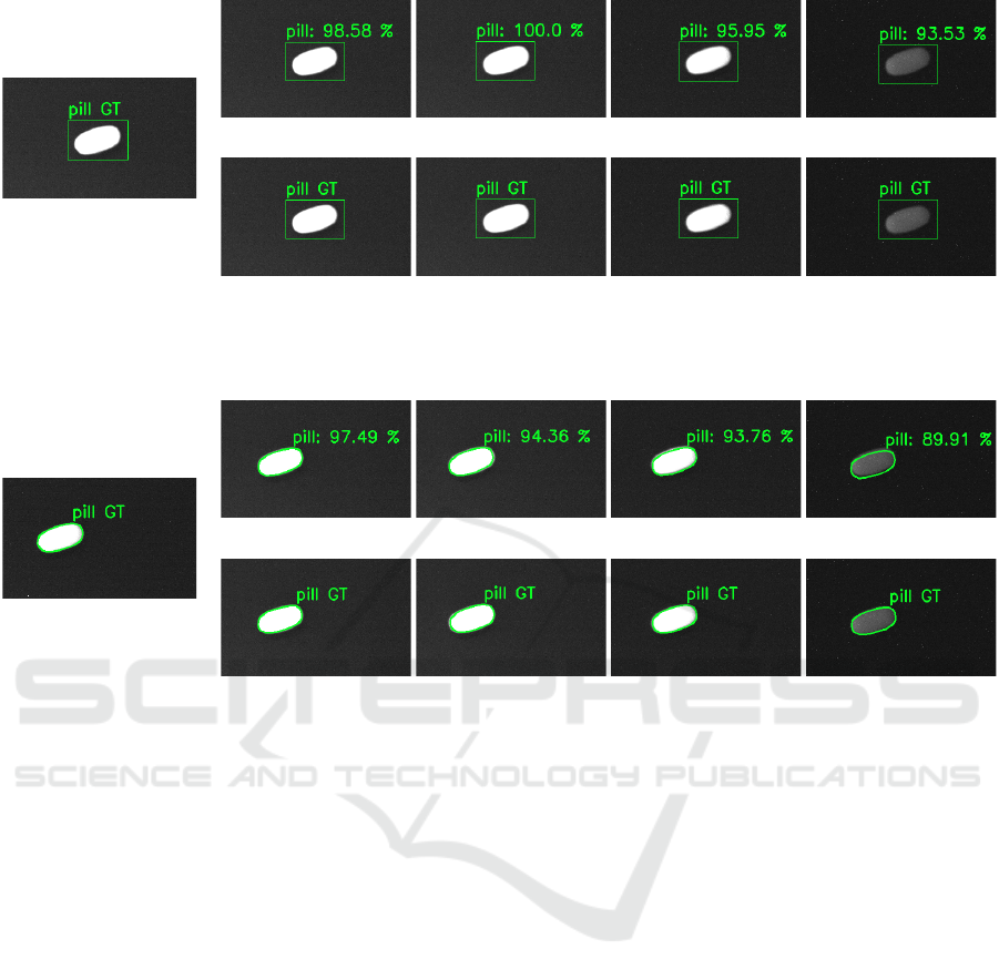
(a) Band 5 input.

(b) Band 1 output. (c) Band 2 output. (d) Band 3 output. (e) Band 4 output.

(f) Band 1 reference. (g) Band 2 reference. (h) Band 3 reference. (i) Band 4 reference.

Figure 2: BB labeled experiment: (a) Reference image (band 5) to start with, (b, c, d, e) Transformed labels (bands 1-4) and

(f, g, h, i) Ground truth labels for comparison purposes (bands 1-4).

(a) Band 5 input.

(b) Band 1 output. (c) Band 2 output. (d) Band 3 output. (e) Band 4 output.

(f) Band 1 reference. (g) Band 2 reference. (h) Band 3 reference. (i) Band 4 reference.

Figure 3: Mask labeled experiment: (a) Reference image (band 5) to start with, (b, c, d, e) Transformed labels (bands 1-4)

and (f, g, h, i) Ground truth labels for comparison purposes (bands 1-4).

band1

BB|mask

· l

RGB

band2

BB|mask

· l

RGB

band3

BB|mask

· l

RGB

band4

BB|mask

· l

RGB

band5

= I

2x3

· l

RGB

(10)

The initial process for generating the im

RGB

[R, G, B] is illustrated in Fig. 4. A combination of

blue (Fig. 4a), green (Fig. 4b) and red (Fig. 4c) im-

ages is performed, generating the artiﬁcial fake RGB

image (Fig. 4d).

Once the artiﬁcial RGB image has been generated,

the objects have been labeled in both the BB format

(Fig. 5a) and the mask format (Fig. 6a). Subse-

quently, the images with BB (Figs. 5b-5f) and masks

(Figs. 6b-6f) were generated by applying the transfor-

mations obtained from Section 3.2. As it can be ob-

served, the results obtained demonstrate the efﬁcacy

of the proposed approach. For instance, the objects in

band 4 with BB (Fig. 5e) and mask (Fig. 6e) labeling

are no longer visible to some extent. However, due

to the method designed, the objects in those positions

are labeled even though they are not visible.

4 CONCLUSION

This work presents a method for automatically la-

belling multispectral images, beginning with a single-

band image BB or mask labeled image.

In order to achieve this, a two-step process is em-

ployed, comprising phase correlation and reﬁnement.

In the initial step, the transformation between the two

images is obtained by applying a Hanning window

to the image, transforming the spatial domain im-

ages into the frequency domain with the Fourier dis-

crete transform, applying the cross-power spectrum

formula to retain just the phase information of the im-

ages, converting the cross-power spectrum back to the

spatial domain, and ﬁnally locating the peak, which

represents the translation between the two analysed

images. The second process entails reﬁning the trans-

formation obtained in the preceding step by searching

Transferability of Labels Between Multilens Cameras

415

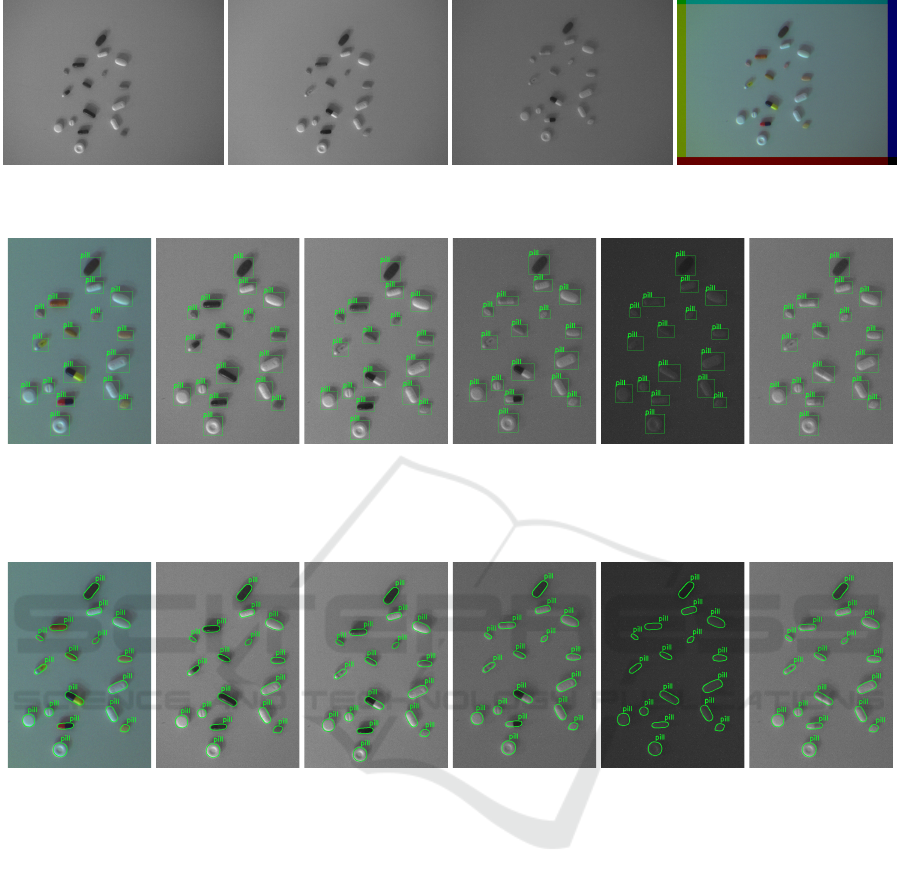
(a) Band 1: blue. (b) Band 2: green. (c) Band 3: red. (d) Fake RGB image.

Figure 4: Combination to create fake RGB images: (a,b,c) Bands 1, 2, 3, respectively and (d) Generated fake RGB image.

(a) Fake RGB

labeled with BBs.

(b) Band 1 with

transfered labels.

(d) Band 3 with

transfered labels.

(e) Band 4 with

transfered labels.

(f) Band 5 with

transfered labels.

Figure 5: BB labeled fake RGB image and transferred labels: (a) Fake RGB image with BB labels and (b,c,d,e,f) Labels

transferred to bands 1-5, respectively.

(a) Fake RGB

labeled with masks.

(b) Band 1 with

transfered labels.

(d) Band 3 with

transfered labels.

(e) Band 4 with

transfered labels.

(f) Band 5 with

transfered labels.

Figure 6: Mask labeled fake RGB image and transferred labels: (a) Fake RGB image with mask labels and (b,c,d,e,f) Labels

transferred to bands 1-5, respectively.

in a proximity window for an optimal one through an

iterative process at the pixel and two subpixel levels,

with the best transformation being saved as the one

that yielded the highest percentage in the IOU index.

In order to test the method, the transformation

between ﬁve multispectral lenses from a MicaSense

RedEdge-MX Dual camera was obtained. By simply

labeling 12 images from band 5 with a high contrast,

it was possible to obtain the transformation of the la-

bel types with an accuracy of 97% and 94% for the

BB and mask label types, respectively, in just 58 ms

and 72 ms. Subsequently, the inverse of the afore-

mentioned transformations was employed to generate

an artiﬁcial RGB image, thereby facilitating the la-

belling process in coloured images. Subsequently, the

labels are transformed back into each lens, thus en-

suring that the labels are present in all ﬁve channels

of the multispectral camera.

Future work will include testing the proposed

method on additional multispectral cameras with dif-

fering morphologies, as well as testing it with all ten

lenses that the camera used in the present paper has.

Furthermore, the integration of an RGB camera would

facilitate the avoidance of the generation of artiﬁcial

RGB images derived from the multispectral lenses,

thereby reducing the potential for the accumulation

of minor errors during the process. An alternative

approach would be to create a dataset of domestic

waste with the aim of training different NNs and test-

ing whether the additional information provided by 10

VISAPP 2025 - 20th International Conference on Computer Vision Theory and Applications

416

lenses and 12-bit images could facilitate more accu-

rate categorisation compared to the same NNs using

8-bit RGB images of objects that resemble the same

but are made of different materials.

ACKNOWLEDGEMENTS

Research work was funded by grant

PID2021-122685OB-I00 funded by MI-

CIU/AEI/10.13039/501100011033 and ERDF/EU.

REFERENCES

Andersson, P., Montan, S., and Svanberg, S. (1987). Mul-

tispectral system for medical ﬂuorescence imaging.

IEEE Journal of Quantum Electronics, 23(10):1798–

1805.

Benjamin, MatvL, midaha, PGibson, RMcKinlay, and Kan,

W. (2016). Dstl satellite imagery feature detection.

Gallagher, J. E., Gogia, A., and Oughton, E. J. (2024). A

multispectral automated transfer technique (matt) for

machine-driven image labeling utilizing the segment

anything model (sam). arXiv preprint.

omez, P. and Meoni, G. (2021). Msmatch: Semisuper-

vised multispectral scene classiﬁcation with few la-

bels. IEEE Journal of Selected Topics in Applied

Earth Observations and Remote Sensing, 14:11643–

11654.

Helber, P., Bischke, B., Dengel, A., and Borth, D. (2019).

Eurosat: A novel dataset and deep learning bench-

mark for land use and land cover classiﬁcation. IEEE

Journal of Selected Topics in Applied Earth Observa-

tions and Remote Sensing, 12(7):2217–2226.

Hoffer, R., Johannsen, C., and Baumgardner, M. (1966).

Agricultural applications of remote multispectral

sensing. In Proceedings of the Indiana Academy of

Science, volume 76, pages 386–396.

Kemker, R., Salvaggio, C., and Kanan, C. (2018). Al-

gorithms for semantic segmentation of multispectral

remote sensing imagery using deep learning. ISPRS

Journal of Photogrammetry and Remote Sensing.

Kirillov, A., Mintun, E., Ravi, N., Mao, H., Rolland, C.,

Gustafson, L., Xiao, T., Whitehead, S., Berg, A. C.,

Lo, W.-Y., et al. (2023). Segment anything. In Pro-

ceedings of the IEEE/CVF International Conference

on Computer Vision, pages 4015–4026.

Lowe, D. G. (1999). Object recognition from local scale-

invariant features. In Proceedings of the seventh

IEEE international conference on computer vision,

volume 2, pages 1150–1157. IEEE.

Ma, F., Yuan, M., and Kozak, I. (2023). Multispectral imag-

ing: Review of current applications. Survey of Oph-

thalmology, 68(5):889–904.

Maxwell, E. L. (1976). Multivariate system analysis of mul-

tispectral imagery. Photogrammetric Engineering and

Remote Sensing, 42(9):1173–1186.

Mia, M. S., Tanabe, R., Habibi, L. N., Hashimoto, N.,

Homma, K., Maki, M., Matsui, T., and Tanaka, T.

S. T. (2023). Multimodal deep learning for rice yield

prediction using uav-based multispectral imagery and

weather data. Remote Sensing, 15(10).

sep, A., Meinhardt, T., Ferroni, F., Peri, N., Ramanan, D.,

and Leal-Taix

e, L. (2024). Better call sal: Towards

learning to segment anything in lidar. arXiv preprint.

aez-Ubieta, I. d. L., Casta

no-Amor

os, J., Puente, S. T., and

Gil, P. (2023). Vision and tactile robotic system to

grasp litter in outdoor environments. Journal of Intel-

ligent & Robotic Systems, 109(2):36.

Park, H. G., Yun, J. P., Kim, M. Y., and Jeong, S. H. (2021).

Multichannel object detection for detecting suspected

trees with pine wilt disease using multispectral drone

imagery. IEEE Journal of Selected Topics in Applied

Earth Observations and Remote Sensing, 14:8350–

8358.

aez-Ubieta, I. d. L., Velasco-S

anchez, E., Puente, S. T.,

and Candelas, F. (2023). Detection and depth esti-

mation for domestic waste in outdoor environments

by sensors fusion. IFAC-PapersOnLine, 56(2):9276–

9281. 22nd IFAC World Congress.

Torralba, A., Russell, B. C., and Yuen, J. (2010). Labelme:

Online image annotation and applications. Proceed-

ings of the IEEE, 98(8):1467–1484.

Ulku, I., Akag

und

uz, E., and Ghamisi, P. (2022). Deep se-

mantic segmentation of trees using multispectral im-

ages. IEEE Journal of Selected Topics in Applied

Earth Observations and Remote Sensing, 15:7589–

7604.

Wang, C.-Y., Bochkovskiy, A., and Liao, H.-Y. M. (2023).

Yolov7: Trainable bag-of-freebies sets new state-

of-the-art for real-time object detectors. In 2023

IEEE/CVF Conference on Computer Vision and Pat-

tern Recognition (CVPR), pages 7464–7475. IEEE.

Wang, X., Zhang, R., Kong, T., Li, L., and Shen, C.

(2020). Solov2: Dynamic and fast instance segmenta-

tion. Advances in Neural information processing sys-

tems, 33:17721–17732.

Yang, Y. and Newsam, S. (2010). Bag-of-visual-words and

spatial extensions for land-use classiﬁcation. In Pro-

ceedings of the 18th SIGSPATIAL international con-

ference on advances in geographic information sys-

tems, pages 270–279.

Yuan, K., Zhuang, X., Schaefer, G., Feng, J., Guan, L., and

Fang, H. (2021). Deep-learning-based multispectral

satellite image segmentation for water body detection.

IEEE Journal of Selected Topics in Applied Earth Ob-

servations and Remote Sensing, 14:7422–7434.

Transferability of Labels Between Multilens Cameras

417