Dynamic Graph Representation with Contrastive Learning for Financial
Market Prediction: Integrating Temporal Evolution and Static Relations
Yunhua Pei
1 a
, Jin Zheng
2 b
and John Cartlidge
2 c
1
School of Computer Science, University of Bristol, U.K.
2
School of Engineering Mathematics and Technology, University of Bristol, U.K.
Keywords:
Contrastive Learning, Financial Market Forecasting, Graph Neural Networks, Temporal Graph Learning.
Abstract:
Temporal Graph Learning (TGL) is crucial for capturing the evolving nature of stock markets. Traditional
methods often ignore the interplay between dynamic temporal changes and static relational structures be-
tween stocks. To address this issue, we propose the Dynamic Graph Representation with Contrastive Learning
(DGRCL) framework, which integrates dynamic and static graph relations to improve the accuracy of stock
trend prediction. Our framework introduces two key components: the Embedding Enhancement (EE) module
and the Contrastive Constrained Training (CCT) module. The EE module focuses on dynamically captur-
ing the temporal evolution of stock data, while the CCT module enforces static constraints based on stock
relations, refined within contrastive learning. This dual-relation approach allows for a more comprehensive
understanding of stock market dynamics. Our experiments on two major U.S. stock market datasets, NAS-
DAQ and NYSE, demonstrate that DGRCL significantly outperforms state-of-the-art TGL baselines. Ablation
studies indicate the importance of both modules. Overall, DGRCL not only enhances prediction ability but
also provides a robust framework for integrating temporal and relational data in dynamic graphs. Code and
data are available for public access.
1 INTRODUCTION
The goal of predicting stock movements attracts much
attention, as success offers the opportunity to gen-
erate substantial investment returns. Previous re-
search can generally be divided according to the in-
put features used in the model. Historical price is
the most common and basic input feature, includ-
ing the open price, close price, highest price, low-
est price, and trading volume (OHLCV). Many pre-
dictions have been made based solely on historical
prices, including applying empirical mode decompo-
sition with factorization machine-based neural net-
works (Zhou et al., 2019) and forming a stochastic re-
current network with seq2seq architecture and atten-
tion mechanism (Wang et al., 2019). More attempts
include adding technical indicators such as achieving
Long Short-Term Memory (LSTM) with the atten-
tion mechanism (Chen and Ge, 2019), creating multi-
task RNNs with high-order Markov random fields (Li
et al., 2019).
a
https://orcid.org/0000-0003-2906-0827
b
https://orcid.org/0000-0002-1783-1375
c
https://orcid.org/0000-0002-3143-6355
Graphs, which represent information through en-
tities, attributes, and their relationships, have recently
gained popularity. This is due to their effectiveness in
illustrating the connections between stocks and their
various attributes. By casting a graph, relevant infor-
mation transfer between stocks and stock attributes
from other channels can be studied. For instance, the
attention mechanism is used to build a market knowl-
edge graph to contain dual-type entities and mixed re-
lationships (Zhao et al., 2022), GCNs with temporal
graph convolution are performed on data in a rolling
window (Matsunaga et al., 2019), and incorporat-
ing emotional factors within a non-stationary Markov
chain model (Liu et al., 2022a). These graph-based
models leverage the structure of GNNs to iteratively
aggregate, showing potentially powerful performance
compared with non-graph-based models.
Although previous research has delved into com-
prehensive investigations of the stock market, several
key issues still need to be solved. The first issue is
forecasting a single time series, which does not cap-
ture the overall market trend and leaves the relation-
ships between stocks and the mechanisms influenc-
ing price transmission unexplored. The second one
298
Pei, Y., Zheng, J. and Cartlidge, J.
Dynamic Graph Representation with Contrastive Learning for Financial Market Prediction: Integrating Temporal Evolution and Static Relations.
DOI: 10.5220/0013154700003890
Paper published under CC license (CC BY-NC-ND 4.0)
In Proceedings of the 17th International Conference on Agents and Artificial Intelligence (ICAART 2025) - Volume 2, pages 298-309
ISBN: 978-989-758-737-5; ISSN: 2184-433X
Proceedings Copyright © 2025 by SCITEPRESS – Science and Technology Publications, Lda.

is that constructing stock market graphs relies heavily
on prior knowledge, and is challenging to adapt au-
tomatically. The third is relations obtained from the
knowledge base are not effectively utilized and are
only used as tools for building graph networks.
To address these limitations, we propose a frame-
work called Dynamic Graph Representation with
Contrastive Learning (DGRCL), which consists of
three main components, namely embedding enhance-
ment, contrastive constrained training, and dynamic
graph evolution. In embedding enhancement, we
adaptively construct dynamic edges that follow Zipf’s
law. Subsequently, the enhanced features are derived
from OHLCV, computed with refined distance calcu-
lations utilizing the Fourier transform. Using these
enhanced features and dynamic edges, we continue to
apply GCNs to these evolving graphs to extract the
latent node embeddings. To further refine the embed-
dings and optimize predictions, we integrate company
relationships as constraints within an adaptive con-
trastive learning module. This module employs con-
trastive loss in the latent space to maximize the con-
sistency between two augmented views of the input
graph, thereby ensuring more robust feature represen-
tation. Finally, our model captures dynamic changes
in the graph over time by employing a time series
forecasting architecture, which can utilize either a
Gated Recurrent Unit (GRU) or LSTM. This enables
DGRCL to generate accurate and temporally-aware
predictions.
To the best of our knowledge, our work is the first
to incorporate stock relations as constraints into con-
trastive learning models for stock prediction, espe-
cially those based on GNNs. The main contributions
of this work can be summarised as follows:
• We adaptively construct dynamic edges that fol-
low the objective laws, refining stock features
through Fourier transform-based distance calcu-
lations. This allows the model to more effec-
tively capture the intricate and dynamic relation-
ships between stocks.
• We integrate company relationships as constraints
within a contrastive learning module, employing
contrastive loss in the latent space to maximize
the consistency between two augmented views of
the input graph. This ensures a robust feature rep-
resentation that reflects the complex interdepen-
dencies among stocks.
• We conduct extensive experiments on real-world
stock data from the US market. We conduct ex-
tensive experiments on real-world stock datasets
with 2,763 stocks from two famous US mar-
kets (NASDAQ and NYSE). The experimental re-
sults demonstrate that DGRCL significantly out-
performs state-of-the-art baselines in predicting
the next trading day movement, with average im-
provements of 2.48% in classification accuracy,
5.53 in F1 score, and 6.67 in Matthew correlation
coefficient.
2 RELATED WORK
2.1 GNNs
GNNs are designed with specific consideration for
tasks involving graph data, such as node classi-
fication, graph classification, and link prediction.
In GALSTM (Yin et al., 2022), an attention-based
LSTM is constructed to learn weight matrices from
Hawkes correlation graphs generated by different
stocks to improve the stock selection winning rate
while paying less attention to the optimal trading
strategy. The most profitable stock prediction is also
one task of portfolio management. Intra-sector rela-
tions, inter-sector relations, and stock-sector relations
are considered in the previous study (Hsu et al., 2021)
to find hierarchical influence among stocks and pre-
dict the most profitable stock. Although sector-level
modeling is performed in their model, some fine-
grained metadata with descriptions of listed company
attributes deserves more attention. Stock description
documents can also be introduced into the model. For
example, Yahoo Finance is one of the channels for
topic-based extraction models in TRAN (Gao et al.,
2021) to make stock recommendations. Similar lim-
itation, TRAN only constructs the stock graph as a
static one. Current approaches need to focus on port-
folio construction and selection, as well as on under-
standing the dynamic interactions between these port-
folios.
2.2 Graph Contrastive Learning
Recently, contrastive representation learning on
graphs has gained significant interest. It contrasts pos-
itive and negative sample pairs, aiming to bring simi-
lar samples closer and push dissimilar ones apart, fo-
cusing on solving the graph manual labeling problem
in the real world. According to (Liu et al., 2022c),
previous research can be categorized into cross-scale
contrasting and same-scale contrasting. Cross-scale
contrasting involves comparing elements at different
scales. For example, MVGRL (Hassani and Khasah-
madi, 2020) takes a multi-view approach by using a
diffused graph as a global view and maximizing MI
across both views and scales. DGI (Velickovic et al.,
2019) contrasts patch-level and graph-level represen-
Dynamic Graph Representation with Contrastive Learning for Financial Market Prediction: Integrating Temporal Evolution and Static
Relations
299

tations by maximizing mutual information, which
helps propagate global information to local represen-
tations. Same-scale contrasting focuses on elements
at the same scale, such as comparing graphs directly.
Within this approach, methods are further divided
into context-based and augmentation-based. Context-
based methods typically use random walks to iden-
tify positive pairs. Augmentation-based methods, like
GraphCL (You et al., 2020), generate positive pairs
through various perturbations at the graph level. GCA
(Zhu et al., 2021) performs node-level augmentations
tailored to the graph’s structure and attributes, while
IGSD (Zhang et al., 2023) uses graph diffusion to cre-
ate augmented views and employs a teacher-student
framework.
3 PRELIMINARY
3.1 Notation
3.1.1 Graph Representation Learning
Let G = (V ,E) denote the graph model where V is
the set of nodes. The length of the time series is T ,
and X
i
∈ R
D×T
is the covariate time-series data as-
sociated with node i, where each node is associated
with D different covariate time series. Furthermore, at
time step t, covariate values for node i is represented
as x
i
t
, and X
i
T
=

x
i
1
,...,x
i
T

is the set of time-series
in graph G. Two different nodes i and j that contain
an edge (i, j) ∈ E without a direction, forming graph
G an undirected one, encoding an explicit dependence
between nodes. Let A ∈ R
N×N
denote this sparse ad-
jacency matrix at a certain time. If (i, j) ∈ E, then A
i j
represents the weight of the edge (dependency) be-
tween node i and j, and A
i j
= 0 when (i, j) /∈ E oth-
erwise. Hence, the graph structure is represented by
the adjacency matrix A and its corresponding time-
series

X
i
T
|i = 1,..., N

.
3.1.2 Graph Contrastive Learning
Given an input Graph G, graph contrastive learn-
ing aims to learn the representations in node-level
tasks in this work by maximizing the feature con-
sistency between two augmented views of the input
graph via contrastive loss in the latent space. Data
augmentation q(·) is a common operation to obtain
two views v
a
and v
b
for the same graph G, includ-
ing node dropping, edge perturbation, subgraph sam-
pling, etc. With these views, latent representations z
a
and z
b
are then extracted by GNNs. Finally, given the
latent representations, a contrastive loss is optimized
to score the positive pairs

z
i
a
,z
i
b

higher compared
to other negative pairs, including inter-view negative
pairs
n
z
i
a
,z
j
b
o
, and intra-view negative pairs
n
z
i
a
,z
j
a
o
.
3.2 Problem Setting
The proposed framework solves the following graph-
based time-series forecasting problem. For all stocks,
a set of stock historical sequence data at day t is rep-
resented by X ∈ R
N×T ×D
, where D is the dimension
of features of one stock, the OHLCV. With a given
lookback window of length δ, the model can make
predictions for the next day’s (t + 1) movements of
the stocks, using the data of X
t−δ:t
. The movement is
calculated by p
t+1
c
− p
t
c
, in which p
t
c
means the close
price of the stock at day t, resulting two prediction
outcomes. A positive result means the price will go
up (label = 1), while a negative result means it will
go down (label = 0), making this a binary classifica-
tion task.
4 METHODOLOGY
In this section, we elucidate the framework of the pro-
posed DGRCL as shown in Fig.1. Given OHLCV of
the stocks in a certain interval [t − δ + 1,t] and the
company relations, we aim to predict the next day’s
stock price movement. First, we construct the stock
graph with envolving edges for different time steps
and generate initial embeddings for each node. Sec-
ond, we extract the dynamic node representations for
each time step. Then, a constraint data augmentation
method is encoded using the company relations. Af-
ter that, we feed the constrained dynamic node rep-
resentations to an RNN-based model to get the final
representation of the nodes. Finally, we predict the
stock movement based on the generated node repre-
sentation from RNNs.
4.1 Embedding Enhancement
4.1.1 Graph Construction
The future performance of a stock is influenced by
its past behavior and its connections to related stocks.
Current research often depends heavily on established
knowledge, such as manual industry classifications
(Huynh et al., 2023; Feng et al., 2019; Xu et al., 2021).
However, this approach can be expensive, relies heav-
ily on empirical experience, and may not generalize
well to new forecasting tasks. In this regard, we fol-
low the data-driven manner in (Wang et al., 2022) to
calculate a proximity function by applying Dynamic
ICAART 2025 - 17th International Conference on Agents and Artificial Intelligence
300

Figure 1: Schematic illustration of DGRCL framework. Top-left: In the process of embedding enhancement, dynamic stock
graphs with enhanced features are generated. Bottom: Then, an encoder is trained with the company relations in a contrastive
manner inside the CCT module, to improve the generation of an initial embedding matrix for the subsequent step. Top-right:
Finally, the layer weights are learned through general RNNs (e.g., GRU, LSTM) to yield the final predictions.
Time Warping (DTW) (Jeong et al., 2011) on the in-
put signals x
i
t
, which will be further introduced in the
experiment part. This process involves utilizing dy-
namic programming on a path matrix to determine
the minimum alignment cost for each pair of stock
sequences x
i
t
and x
j
t
with a lookback window δ:
cost(x
i
t
,x
j
t
) ⇐= DTW (x
i
t−δ:t
,x
j
t−δ:t
) (1)
In DGRCL, we set the time step as 1. Through
computations for each pair of stock sequences within
the same time step, a corresponding cost matrix
˙
A
t
is
generated for that particular time step t, and the total
number of the cost matrices is T − δ.
Traditional methods typically employ a hard
threshold to partition the cost matrix
˙
A
t
and form the
adjacency matrix A
t
of the graph (Wang et al., 2022).
However, such approaches are often subjective. The
adjacency matrix, which represents the edges in a
graph, heavily relies on the structural information of
its edges for information transmission. Hence, we in-
troduce an adaptive method to estimate the number of
significant edges that a graph should possess based on
the number of nodes it contains.
According to (Sawhney et al., 2021b), the scale-
free structure of stock graphs is characterized by a
power-law distribution in node degrees, at least in
an asymptotic sense. Specifically, the fraction P(n)
of nodes in the graph having n connections to other
nodes follows the distribution (Barab
´
asi and Albert,
1999), where s is the exponent.
P(n) ∼ n
−s
(2)
This observation can be explained by Zipf’s law
(Newman, 2005), an empirical principle that tends to
hold approximately when a list of measured values
is sorted in descending order. The probability mass
function of the Zipf distribution is a discrete proba-
bility distribution as,
P(X = n) =
n
−s
∑
N
i=1
(i
−s
)
(3)
where N is the total number of possible outcomes,
n is a specific outcome. Then we can give the expec-
tation of a random variable X with a Zipf distribution
using the formula:
E(X) =
∑
N
n=1
n · P(X = n) (4)
It should be noted that when applied, n will rep-
resent the count of known nodes, signifying the num-
ber of stocks in the stock graph. This approach al-
lows us to provide a rough estimate of the expected
number of edges E(n) in a stock network based on a
given number of nodes n. Then, by employing a bi-
nary classification method, we manage the number of
values exceeding the threshold to remain below the
specified limit E(n). This enables us to dynamically
construct edges to build a stock graph G. Further-
more, we obtain the dynamic graph for each time step
as G
1
,G
2
...G
T −δ
.
4.1.2 Feature Optimization
Statistical properties such as mean and variance in
time series data often change over time, leading to dis-
Dynamic Graph Representation with Contrastive Learning for Financial Market Prediction: Integrating Temporal Evolution and Static
Relations
301

tribution shift problems (Du et al., 2021; Kim et al.,
2021). This change in time distribution poses a sig-
nificant challenge in stock series to achieving accu-
rate time series forecasting. Therefore, we need to
enhance the input stock series.
To identify the distribution characteristics of a
time series, it needs to be transformed into another
domain, such as the frequency domain. The Fourier
transform (FT) (Cochran et al., 1967; Bloomfield,
2004) is an integral transform that presents a func-
tion into a representation that emphasizes the origi-
nal function, which has wide applications in physics,
mathematics, and engineering.
Here, we apply the Fast Fourier Transformation
(FFT) (Cochran et al., 1967) to one stock series, and
follow the temporal distribution characterization in
(Du et al., 2021), with the principle of maximum en-
tropy (Jaynes, 1982) to find the most dissimilar peri-
ods, whose objective can be formulated as:
max
0<k≤k
0
max
n
1
,...,n
k
1
k
∑
1<i̸= j≤k
d(FFT (x
i
),FFT (x
j
)) (5)
s.t.∀i,△
1
<


x
i


< △
2
;
∑
i


x
i


= X
i
∈ R
D×T
(6)
where d(·) is a distance metric, k
0
is the hyperpa-
rameter to avoid over-splitting, and △
1
,△
2
are pre-
defined parameters to avoid trivial solutions (e.g., ex-
tremely small or large values might not effectively
capture the distribution information). T is the length
of time-series and D is the dimension of features.
The metric d(·) can be any distribution distance cal-
culations such as Euclidean, JS-divergence, and KL-
divergence. By searching k, the corresponding peri-
ods, and then applying this approach to each feature
dimension d, we can find the most dissimilar period
pairs in the feature domain for the stock. By perform-
ing similar operations on each stock, we obtain the
enhanced stock graph node embedding matrix X
′
.
It’s important to notice that in one stock series, the
sequences derived from FFT transformation in both
rising and falling markets exhibit similarity, details
please refer the experiments. The distinguishing fac-
tor lies in the fluctuating market. Therefore, we will
generate three sets of results (rising, falling, and fluc-
tuating) to serve as enhanced representations x
′
i
of
one feature for stock i.
4.2 Contrastive Constrained Training
In previous stock prediction methods, company rela-
tions are mainly used to define the edge structure of
stock graphs for information propagation (Feng et al.,
2019; Kim et al., 2019). Consideration of these rela-
tions as a constraint has been largely ignored during
the training process. Therefore, we propose a Con-
trastive Constrained Training (CCT) module that inte-
grates company relations to learn a constrained GNN
encoder through contrastive learning. We will begin
by introducing the adaptive constrained augmenta-
tion, followed by the contrastive learning framework,
as the two components of the CCT module.
4.2.1 Adaptive Constrained Augmentation
Contrastive learning methods, which aim to maximize
agreement between views, strive to learn representa-
tions consistent despite perturbations introduced by
augmentation techniques. Within the CCT module,
we propose an adaptive enhancement scheme based
on company relation constraints. The aim is designed
to disrupt less important links and features while pro-
tecting the important constraint structure and proper-
ties.
In this step, contrary to previous methods, we
incorporate company relations as constraints dur-
ing training, resulting in a reevaluation of the for-
mer stock graph. The probability of the edge be-
tween node i, j remains in the augmentation step
P
{
(i, j) ∈ E
}
is calculated as:
1 − min

logw
max
− log w
logw
max
− log w
µ
e · p
e
, p
τ

(7)
where w is the average of the degree centrality
(Newman, 2018) between node i and j. We first cal-
culate w for all edges and then make a max-mean nor-
malization using the max and mean (µ). To balance
the probabilities, we then take the logarithm of the
result. p
e
and p
τ
are hyperparameters to control the
overall probability of removing edges and the cut-off
threshold.
The key approach presented in CCT is that the
degree centrality calculation method is based on the
company relation of the stocks, rather than the edges
within the stock graph. That is, given the stock rela-
tion encodings A and each kind of relation A
relation
i j
∈
A for node pair (i, j) we must adhere to the constraint
that there must be at least one type of relation that
exists A
relation
i j
> 0. With this constraint, we can cal-
culate w using the following method.
1
2
∑
(i, j)∈E
A
relation
ji
+
∑
(i, j)∈E
A
relation
i j
!
(8)
After calculating the edge remaining probability,
we generate two views for the input graph G to per-
form contrastive learning.
ICAART 2025 - 17th International Conference on Agents and Artificial Intelligence
302

4.2.2 Contrastive Learning Framework
The proposed CCT module follows the common
graph contrastive learning paradigm, in which the
model aims to maximize the alignment of repre-
sentations across various perspectives (Hassani and
Khasahmadi, 2020; Zhu et al., 2021). We initially cre-
ate two different views of the graph G, by applying
adaptive constrained augmentation to the input. Sub-
sequently, we utilize a contrastive objective function
that ensures the encoded embeddings of each node in
these two distinct views align with each other, while
also being distinguishable from embeddings of other
nodes.
Specifically, during each training epoch, the CCT
module begins by randomly selecting two data aug-
mentation functions from q(·), which is a common
operation to obtain two views v
a
∼ q(G), v
b
∼ q(G),
then, node representations z
a
and z
b
are obtained from
a GNN encoder g(·). For a given node i, its embed-
ding z
i
a
generated in view v
a
serves as the anchor,
while the embedding of it generated in the other view
z
i
b
forms the positive sample, and the remaining em-
beddings in the two views are considered as nega-
tive samples. Following (Zhu et al., 2021), we define
the pairwise objective ℓ(z
i
a
,z
i
b
) for each positive pair
(z
i
a
,z
i
b
) as :
log
e
θ(z
i
a
,z
i
b
)/τ
e
θ(z
i
a
,z
i
b
)/τ
+
∑
e
θ(z
i
a
,z
j
b
)/τ
+
∑
e
θ(z
i
a
,z
j
a
)/τ
(i ̸= j) (9)
where τ is a temperature parameter, and e
θ(z
i
a
,z
i
b
)/τ
represent positive pair.
∑
e
θ(z
i
a
,z
j
b
)/τ
,
∑
e
θ(z
i
a
,z
j
a
)/τ
mean
inter-view negative pairs and intra-view negative
pairs. θ(z
a
,z
b
) = s(φ(z
a
),φ(z
b
)), in which, s(·) refers
to the cosine similarity and φ(·) is a non-linear projec-
tion, implemented as a two-layer perception model.
Moreover, the overall objective L
cl
for the CCT mod-
ule to be maximized uses the average for all positive
pairs, since the two views are symmetric.
L
cl
=
1
2N
N
∑
i=1
(ℓ(z
i
a
,z
i
b
) + ℓ(z
i
b
,z
i
a
)) (10)
In this way, we use the number of relationships as
a basis for measuring the possibility of the existence
of a certain edge, thereby achieving adaptive data aug-
mentation with constraints, which is then trained to-
gether with the dynamic graph evolution.
4.3 Dynamic Graph Evolution
Using dynamic graphs and node embedding matrices,
we will now explain how to acquire the dynamic la-
tent representations of nodes. This process consists
of two components: the graph convolutional network
and the weight evolution.
Based on GCN (Kipf and Welling, 2017), we pro-
pose the following propagation rules:
H
(l+1)
t
= σ(
b
A
t
H
(l)
t
W
(l)
t
) (11)
Here, at time t, the l-th layer takes the adjacency
matrix A
t
and the node embedding matrix H
(l)
t
as
input, and outputs H
(l+1)
t
using a layer-specific train-
able weight matrix W
(l)
t
to update. Specifically, σ(·)
denotes an activation function.
b
A =
e
D
−
1
2
e
A
e
D
−
1
2
,
e
A = A + I ,
e
D = diag
∑
j
e
A
i j
!
(12)
To acquire the dynamic latent representations, the
trainable weight matrix W
(l)
t
, we follow the method-
ology outlined in (Pareja et al., 2020). W
(l)
t
is treated
as the hidden state of the dynamical system updated
by any RNN-based model f (·), such as LSTM and
GRU, with a prediction loss L
pred
.
W
(l)
t
= f (H
(l)
t
,W
(l)
t−1
) (13)
The final prediction result will be derived from the
output of W at the final time step. This result is bina-
rized and then mapped through a so f tmax function to
predict each stock. The final form of the loss function
is shown below, where λ is a trade-off parameter.
L = L
pred
+ λL
cl
(14)
5 EXPERIMENT
In this section, we describe the experimental setup
used to evaluate the effectiveness of our proposed
method. Experimental results demonstrate the effec-
tiveness of our DGRCL framework in comparison
with different backbones and datasets. We specifi-
cally aim to answer the following questions: (RQ1):
How effective is the proposed DGRCL framework for
the graph classification task? (RQ2): How effec-
tive are the individual modules proposed in DGRCL?
(RQ3): How does sensitivity to hyperparameters af-
fect the performance of the proposed model?
5.1 Dataset
We closely follow the experimental setup outlined in
Feng et al. (2019), using two major US stock markets.
Dynamic Graph Representation with Contrastive Learning for Financial Market Prediction: Integrating Temporal Evolution and Static
Relations
303

Table 1: Data statistics of NASDAQ and NYSE.
Item
NASDAQ dataset NYSE dataset
Train Valid Test Train Valid Test
Time Span 01/02/2013-12/08/2017 01/02/2013-12/08/2017
Valid Trading Days 611 94 236 611 94 236
Data Points 5 (OHLCV) 5 (OHLCV)
Nodes 1026 1737
Edges 164 255
Relation Types 112 130
Many studies have utilized this same dataset to eval-
uate their stock forecasting models (Kim et al., 2019;
Sawhney et al., 2021a; Hsu et al., 2021; You et al.,
2024a,b), and to ensure easier comparison with the
existing literature, we also adopt this dataset in our
experiments.
Dataset statistics are summarized in Table 1. We
follow the setup of (Pareja et al., 2020) and divide
the two datasets into training, validation, and testing
sets in the proportions of 0.65, 0.1, and 0.25, respec-
tively. This results in 611, 94, and 236 effective trad-
ing days for each set. OHLCV are daily values for
each stock. Edges number is calculated by (4) with
a certain number of nodes. Recognizing that stocks
within the same industry tend to be similarly affected
by industry-wide prospects, we gather data on the
sector-industry relationships among stocks. For two
datasets, we apply the sector-industry relations as Re-
lation Types in Table 1, for more details, please refer
to (Feng et al., 2019). The dataset and source code are
available in github.
1
Each stock market dataset spans four years, ex-
ceeding one thousand time points, with more than
one thousand traded stocks in each market. Com-
pared to the datasets used in the baseline models, the
datasets employed in DGRCL are characterized by
their long duration, multiple nodes, and dynamic tem-
poral graph changes. This makes financial datasets
particularly well-suited for studying long-term infor-
mation propagation in GNNs, as compared to other
datasets.
5.2 Model Setting
All experiments are performed on a Nvidia GeForce
RTX 3090 graphic card, CUDA version 11.5. The
lookback window δ applied in DTW (·) is 20. In
general, each month consists of approximately 22.5
working days. The input signals x
i
t
for DTW is
the volume volatile, by calculating vol
t
/vol
t−1
. The
RNN-based model f (·) is a two-layer LSTM, follow-
ing the methodology outlined in Pareja et al. (2020).
Three hyperparameters in the CCT module are τ, p
e
,
and p
τ
. Following the work of Zhu et al. (2021), we
1
https://github.com/PEIYUNHUA/DGRCL
set τ as 0.4. For the other two, we train the model us-
ing p
e
and p
τ
from 0.1 to 0.9 with increments of 0.2.
The activation function σ(·) is set to ReLU(·). Based
on the method outlined in Liu et al. (2022b), we con-
trol the trade-off parameter λ to bring L
pred
and L
cl
to
the same order of magnitude. The empirical value of
λ obtained from multiple experiments is 0.1.
5.3 Baseline
We consider state-of-the-art dynamic graph node clas-
sification models as baseline methods to learn the
representations of nodes in a graph, including Graph
WaveNet (Wu et al., 2019), MTGODE (Jin et al.,
2022), STGCL (Liu et al., 2022b), and Evolvegcn
(Pareja et al., 2020).
• Graph WaveNet (Wu et al., 2019): A spatiotempo-
ral graph modeling approach that captures spatial-
temporal dependencies across multiple time se-
ries by integrating graph convolution with dilated
causal convolution. Two datasets are used, the
METR-LA dataset spans four months of traffic
speed data from 207 sensors, while the PEMS-
BAY dataset covers six months from 325 sensors,
both aggregated into 5-minute intervals.
• MTGODE (Jin et al., 2022): A continuous model
that forecasts multivariate time series by inte-
grating dynamic graph neural Ordinary Differen-
tial Equations to unify spatial-temporal message
passing and enhance latent spatial-temporal dy-
namics. The evaluation involves five benchmark
datasets: three conventional time series datasets
(Electricity, Solar-Energy, Traffic) and two traf-
fic datasets (Metr-La, Pems-Bay) with predefined
graph structures and specific time spans.
• STGCL (Liu et al., 2022b): A study that inte-
grates contrastive learning into spatio-temporal
graph (STG) forecasting, leveraging novel node
and graph-level contrastive tasks to mitigate data
scarcity, enhancing performance through joint
learning schemes and strategic data augmenta-
tions. The model is tested using two traffic bench-
marks, PEMS-04 and PEMS-08, with aggregated
5-minute traffic flow, average speed, and occu-
pancy data, applying Z-score normalization and
Gaussian kernel adjacency matrices.
• EvolveGCN (Pareja et al., 2020): An approach to
dynamic graph representation learning that adapts
graph convolutional networks over time by evolv-
ing GCN parameters with recurrent neural net-
works, without relying on node embeddings. The
benchmark datasets include the Stochastic Block
Model (SBM) for simulating community struc-
ICAART 2025 - 17th International Conference on Agents and Artificial Intelligence
304

Table 2: Performance of proposed DGRCL and other baselines on next trading day stock trend classification over the test
period. Bold denotes the best result.
Methods
NASDAQ dataset NYSE dataset
Accuracy(%) F1 score MCC(×10
−3
) Accuracy(%) F1 score MCC(×10
−3
)
Graph WaveNet (Wu et al., 2019) 50.94±0.15 60.51±1.10 5.50±1.00 50.86±0.13 57.28±1.86 11.12±2.21
MTGODE (Jin et al., 2022) 51.41±0.15 62.41±4.24 5.92±2.61 52.35±0.17 62.73±1.72 20.62±5.76
STGCL (Liu et al., 2022b) 50.56±0.08 57.81±1.19 9.71±1.15 51.21±0.05 67.47±0.07 22.33±1.53
EvolveGCN (Pareja et al., 2020) 50.19±0.02 56.94±0.21 4.41±0.76 51.14±0.15 66.85±0.37 14.41±0.45
DGRCL (Ours) 53.06±0.18 66.53±2.74 9.32±1.53 54.07±0.20 67.53±0.19 27.51±5.52
Table 3: Ablation study on the two datasets. We replace the Embedding Enhancement module and Contrastive Constrained
Training module in DGRCL with their discrete implementations, denoted w/o EE and w/o CCT. We further remove all
proposed modules except dynamic graphs for training as w/o EE & CCT.
Methods
NASDAQ dataset NYSE dataset
Accuracy(%) F1 score MCC(×10
−3
) Accuracy(%) F1 score MCC(×10
−3
)
DGRCL 53.06±0.18 66.53±2.74 9.32±1.53 54.07±0.20 67.53±0.19 27.51±5.52
w/o EE 51.45±0.03 62.48±1.19 4.69±0.02 52.77±0.05 62.95±1.40 21.88±2.35
w/o CCT 52.69±0.32 65.61±0.22 5.78±1.07 53.87±0.11 67.34±0.18 23.12±1.77
w/o EE & CCT 51.08±0.12 57.43±1.22 2.91±0.26 51.65±0.21 64.12±0.19 7.61±2.11
tures, Bitcoin OTC (BC-OTC) and Bitcoin Al-
pha (BC-Alpha) for rating predictions, UC Irvine
messages (UCI) for link prediction, and several
other networks for various predictive tasks.
5.4 Evaluation Metric
Following the approaches taken in previous studies
(You et al., 2024a; Kim et al., 2019; Deng et al., 2019;
Sawhney et al., 2020), we assess our result using Clas-
sification Accuracy, F1 score, and Matthews Corre-
lation Coefficient (MCC) to evaluate model perfor-
mance. For all three metrics, higher values indicate
better model performance. We record the time taken
for each training epoch of the models in seconds.
5.5 Evaluation Result
5.5.1 RQ1. Performance Comparison
The experimental results in Table 2 show that our
model outperforms all other baseline models in terms
of accuracy and F1 score, and is also comparable
to the baseline models in terms of MCC. For the
NASDAQ dataset, DGRCL achieves the highest ac-
curacy at 53.06%, surpassing the second-best MT-
GODE by 1.65%. Additionally, DGRCL attains the
top F1 score of 66.53% and a strong MCC value of
9.32, nearly matching the best MCC of 9.71. On the
NYSE dataset, DGRCL similarly outperforms other
methods, with an accuracy of 54.07%, an F1 score of
67.53%, and a substantial MCC of 27.51, marking the
highest recorded metrics across all models. The no-
table discrepancy where MTGODE exhibits a high F1
score but a lower MCC indicates the model may han-
dle accuracy and recall well for the majority class but
struggles with the minority class, affecting its overall
prediction quality. A similar finding is also shown in
the performance of EvolveGCN on the NYSE dataset.
Moreover, we observe that the accuracy of all
baseline methods is not very high, being only slightly
better than 50%, which deviates significantly from
the experimental results described in their respective
papers. A reasonable explanation for this inconsis-
tency is that the nodes and the temporal span of their
datasets are relatively small. As a result, their models
may be unable to effectively learn the representations
of large-scale graph models over long time series. For
instance, in the datasets used by Graph WaveNet and
STGCL, the number of nodes is 207 and 325, respec-
tively, which is far smaller than the 1026 and 1737
nodes in our dataset. Similarly, in the dataset used by
MTGODE, the largest sample size is 52,560, which
is much smaller than the smallest sample size in our
study 626,886 (1026×611).
5.5.2 RQ2. Ablation Study
To verify the effectiveness of each component of
DGRCL, we conducted ablation studies on the two
datasets (see Table 3). The complete DGRCL model
incorporates EE and CCT, exhibiting the highest per-
formance in all metrics. When both EE and CCT are
removed (w/o EE & CCT), DGRCL has the most sig-
Dynamic Graph Representation with Contrastive Learning for Financial Market Prediction: Integrating Temporal Evolution and Static
Relations
305

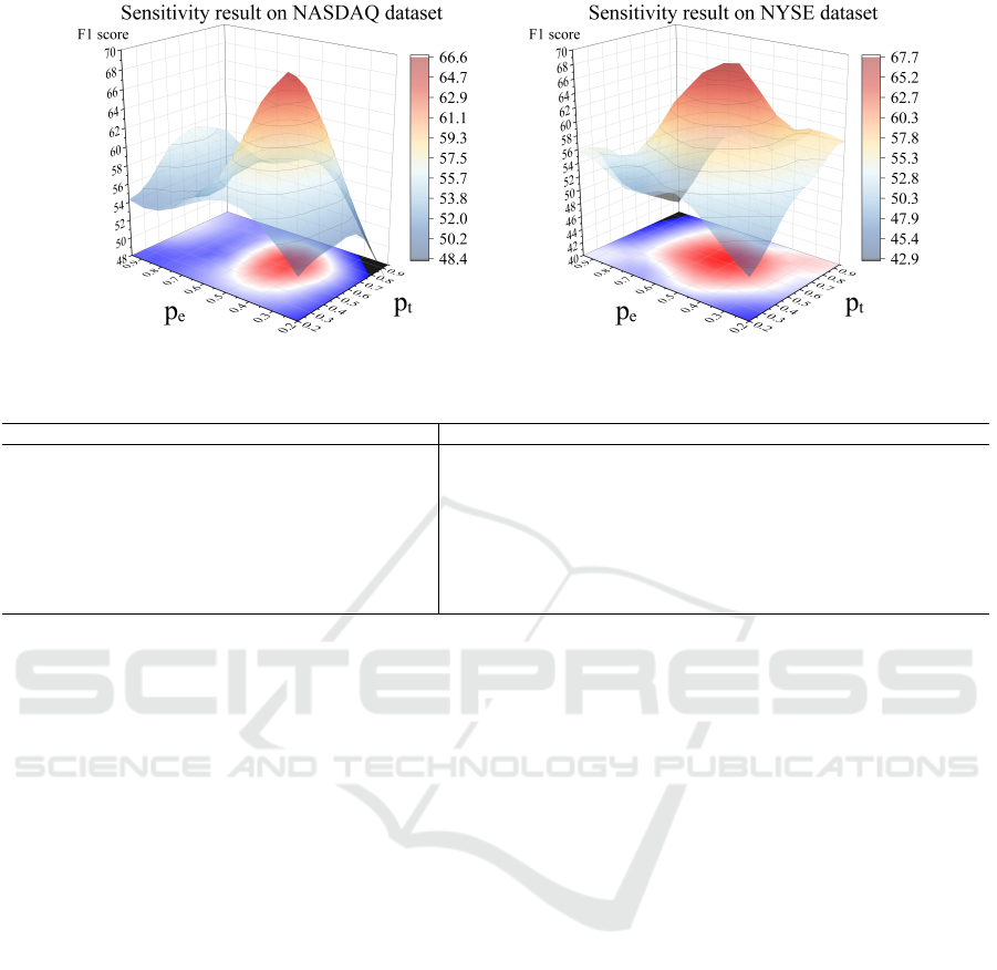
Figure 2: Sensitivity study of the overall probability of removing edges p
e
and the cut-off threshold p
τ
via F1 score.
Table 4: Run-time complexity of the experiments.
Model Dataset Epoch Training Time (s) Model Dataset Epoch Training Time (s)
Graph WaveNet NASDAQ 1.63 DGRCL (Ours) w/o EE NASDAQ 406.53
NYSE 3.14 NYSE 485.38
MTGODE NASDAQ 13.22 DGRCL (Ours) w/o CCT NASDAQ 42.58
NYSE 29.96 NYSE 96.43
STGCL NASDAQ 2.12 DGRCL (Ours) w/o EE & CCT NASDAQ 41.79
NYSE 3.17 NYSE 80.06
EvolveGCN NASDAQ 24.63 DGRCL (Ours) NASDAQ 414.05
NYSE 38.25 NYSE 505.54
nificant performance drop, with accuracy falling to
51.08% and 51.65%, the F1 score to 57.43 and 64.12,
and the MCC to 2.91 and 7.61 in the NASDAQ and
NYSE datasets respectively.
From the result we can find that, by incorporating
the EE module, DGRCL experiences a significant im-
provement, nearly doubling the MCC score on both
datasets. This indicates that the EE module enables
the model to learn more effective latent features of the
time series, thereby enhancing its predictive perfor-
mance. Another observation is that the CCT module
alone does not result in a significant improvement in
model performance and is less effective compared to
adding the EE module alone. Nonetheless, when both
modules are combined, they greatly enhance the over-
all performance of the model. This suggests that the
model achieves optimal predictive results by learning
the dynamic temporal relationships and the static re-
lationships in the graph data.
5.5.3 RQ3. Hyperparameter Sensitivity
We explore the sensitivity of two important hyperpa-
rameters: the overall probability of removing edges
p
e
and the cutoff threshold p
τ
. These two hyperpa-
rameters directly affect the performance of the CCT
module and further impact the overall performance
of the DGRCL. Here, we use the global evaluation
metric F1 score to reflect the overall performance of
different combinations of these hyperparameters. Re-
sults are presented in Fig. 2. We make the following
observations.
When both p
e
and p
τ
are set at their maximum or
minimum values simultaneously, overall performance
is poor, with the F1 score in both datasets falling be-
low 50. This indicates that finding a balance between
these two hyperparameters is crucial to improving the
model’s predictive performance. The second finding
is that p
e
is more important than p
τ
, as it determines
the dynamic lower bound in Eq. (7). If p
τ
is set very
low, P
{
(i, j) ∈ E
}
becomes a fixed value equal to
1 − p
τ
. This indicates that all edges have the same
existence probability, resulting in random remaining.
Another observation is that, Compared to the NAS-
DAQ dataset, the NYSE dataset has a larger optimal
hyperparameter space, making it easier to find local
optima during model training. Previous financial pa-
pers (Lian et al., 2022; Jiang et al., 2011) also support
this finding, noting that the NASDAQ market is more
volatile, leading to a smaller optimal hyperparameter
space.
5.5.4 Complexity
Table 4 compares the training times per epoch (in sec-
onds) of various models on the NASDAQ and NYSE
datasets. Our model, DGRCL, generally has signifi-
cantly higher training times compared to other mod-
els. For example, Graph WaveNet and STGCL re-
quire only 1.63s and 2.12s per epoch on NASDAQ,
ICAART 2025 - 17th International Conference on Agents and Artificial Intelligence
306

respectively, while DGRCL without embedding en-
hancement (EE) and contrastive constrained train-
ing (CCT) takes 41.79s. The full DGRCL model,
which includes these enhancements, requires 414.05s
on NASDAQ and 505.54s on NYSE.
Notably, adding the CCT unit significantly in-
creases the training time, accounting for around 90%
of the total run-time, which indicates that the graph
contrastive learning component is the main source
of computational overhead. However, as shown in
the comparison between Table 2 and Table 3, even
without the CCT module, DGRCL still outperforms
the baselines in terms of accuracy. This demon-
strates that our framework performs well without re-
lying on the computationally expensive CCT mod-
ule. While DGRCL offers improved prediction per-
formance, this high computation cost, particularly
from the CCT module, suggests a need for further
optimization to balance performance and efficiency,
especially in large-scale applications.
6 CONCLUSION
In this paper, we propose the Dynamic Graph Repre-
sentation with Contrastive Learning (DGRCL) frame-
work, which unifies dynamic temporal graph learn-
ing and static relational graph learning through a con-
trastive learning paradigm. Within DGRCL, both the
Embedding Enhancement (EE) and Contrastive Con-
strained Training (CCT) modules complement each
other: the EE module dynamically captures evolv-
ing stock market trends, while the CCT module lever-
ages static inter-stock relationships to refine feature
representations through contrastive learning. This
dual approach enhances the model’s ability to predict
stock movements with higher accuracy. Addition-
ally, we utilize objective laws to construct dynamic
graph structures. Meanwhile, we integrate a Fourier
transform-based technique into the EE module to ef-
fectively address the challenges posed by distribution
shifts in time series data. Ultimately, we validate
the effectiveness of DGRCL through extensive exper-
iments on two real-world datasets, demonstrating that
DGRCL consistently outperforms four baseline mod-
els.
For future work, we will also refine the CCT mod-
ule to better distinguish between static and dynamic
graph features. We will perform comparisons with
additional baselines on financial market datasets from
various countries (such as the Shanghai Stock Ex-
change in China) to further demonstrate the superi-
ority of the DGRCL framework as a long-term time-
series forecasting model for financial predictions. In
addition, to make our framework more efficient, fu-
ture work will focus on optimizing the graph con-
trastive learning part to reduce its computational over-
head and enhance the overall performance of the
DGRCL framework.
ACKNOWLEDGEMENTS
This work was supported by UKRI EPSRC Grant
No. EP/Y028392/1: AI for Collective Intelligence
(AI4CI), and Innovate UK Project No. 10094067:
Stratlib.AI - A Trusted Machine Learning Platform
for Asset and Credit managers. The authors have no
conflicts of interest to declare.
REFERENCES
Barab
´
asi, A.-L. and Albert, R. (1999). Emergence of scal-
ing in random networks. Science, 286(5439):509–
512.
Bloomfield, P. (2004). Fourier analysis of time series: An
introduction. John Wiley & Sons.
Chen, S. and Ge, L. (2019). Exploring the attention mech-
anism in LSTM-based Hong Kong stock price move-
ment prediction. Quantitative Finance, 19(9):1507–
1515.
Cochran, W. T., Cooley, J. W., Favin, D. L., Helms, H. D.,
Kaenel, R. A., Lang, W. W., Maling, G. C., Nelson,
D. E., Rader, C. M., and Welch, P. D. (1967). What is
the fast Fourier transform? Proceedings of the IEEE,
55(10):1664–1674.
Deng, S., Zhang, N., Zhang, W., Chen, J., Pan, J. Z., and
Chen, H. (2019). Knowledge-driven stock trend pre-
diction and explanation via temporal convolutional
network. In Companion Proceedings of The 2019
World Wide Web Conference, pages 678–685.
Du, Y., Wang, J., Feng, W., Pan, S., Qin, T., Xu, R.,
and Wang, C. (2021). AdaRNN: Adaptive learning
and forecasting of time series. In Proceedings of the
30th ACM international conference on information &
knowledge management, pages 402–411.
Feng, F., He, X., Wang, X., Luo, C., Liu, Y., and Chua,
T.-S. (2019). Temporal relational ranking for stock
prediction. ACM Transactions on Information Systems
(TOIS), 37(2):1–30.
Gao, J., Ying, X., Xu, C., Wang, J., Zhang, S., and Li,
Z. (2021). Graph-based stock recommendation by
time-aware relational attention network. ACM Trans-
actions on Knowledge Discovery from Data (TKDD),
16(1):1–21.
Hassani, K. and Khasahmadi, A. H. (2020). Contrastive
multi-view representation learning on graphs. In In-
ternational Conference on Machine Learning, pages
4116–4126.
Hsu, Y.-L., Tsai, Y.-C., and Li, C.-T. (2021). FinGAT: Fi-
nancial graph attention networks for recommending
Dynamic Graph Representation with Contrastive Learning for Financial Market Prediction: Integrating Temporal Evolution and Static
Relations
307

top-k profitable stocks. IEEE Transactions on Knowl-
edge and Data Engineering, 35(1):469–481.
Huynh, T. T., Nguyen, M. H., Nguyen, T. T., Nguyen,
P. L., Weidlich, M., Nguyen, Q. V. H., and Aberer,
K. (2023). Efficient integration of multi-order dynam-
ics and internal dynamics in stock movement predic-
tion. In Proceedings of the Sixteenth ACM Interna-
tional Conference on Web Search and Data Mining,
pages 850–858.
Jaynes, E. T. (1982). On the rationale of maximum-entropy
methods. Proceedings of the IEEE, 70(9):939–952.
Jeong, Y.-S., Jeong, M. K., and Omitaomu, O. A. (2011).
Weighted dynamic time warping for time series clas-
sification. Pattern Recognition, 44(9):2231–2240.
Jiang, C. X., Kim, J.-C., and Wood, R. A. (2011). A com-
parison of volatility and bid–ask spread for NASDAQ
and NYSE after decimalization. Applied Economics,
43(10):1227–1239.
Jin, M., Zheng, Y., Li, Y.-F., Chen, S., Yang, B., and Pan,
S. (2022). Multivariate time series forecasting with
dynamic graph neural ODEs. IEEE Transactions on
Knowledge and Data Engineering, 35(9):9168–9180.
Kim, R., So, C. H., Jeong, M., Lee, S., Kim, J., and Kang,
J. (2019). HATS: A hierarchical graph attention net-
work for stock movement prediction. arXiv preprint
arXiv:1908.07999.
Kim, T., Kim, J., Tae, Y., Park, C., Choi, J.-H., and Choo,
J. (2021). Reversible instance normalization for accu-
rate time-series forecasting against distribution shift.
In International Conference on Learning Representa-
tions.
Kipf, T. N. and Welling, M. (2017). Semi-supervised clas-
sification with graph convolutional networks. In Inter-
national Conference on Learning Representations.
Li, C., Song, D., and Tao, D. (2019). Multi-task recur-
rent neural networks and higher-order Markov random
fields for stock price movement prediction: Multi-task
RNN and higher-order MRFs for stock price classi-
fication. In Proceedings of the 25th ACM SIGKDD
International Conference on Knowledge Discovery &
Data Mining, pages 1141–1151.
Lian, Y.-M., Jhong, Y.-J., Wang, P.-H., and Chen, W.-M.
(2022). An empirical examination of VIX market fluc-
tuations. Advances in Management and Applied Eco-
nomics, 12(4):1–6.
Liu, C., Yan, J., Guo, F., and Guo, M. (2022a). Forecast-
ing the market with machine learning algorithms: an
application of NMC-BERT-LSTM-DQN-X algorithm
in quantitative trading. ACM Transactions on Knowl-
edge Discovery from Data (TKDD), 16(4):1–22.
Liu, X., Liang, Y., Huang, C., Zheng, Y., Hooi, B., and Zim-
mermann, R. (2022b). When do contrastive learning
signals help spatio-temporal graph forecasting? In
Proceedings of the 30th international conference on
advances in geographic information systems, pages 1–
12.
Liu, Y., Jin, M., Pan, S., Zhou, C., Zheng, Y., Xia, F., and
Philip, S. Y. (2022c). Graph self-supervised learning:
A survey. IEEE transactions on knowledge and data
engineering, 35(6):5879–5900.
Matsunaga, D., Suzumura, T., and Takahashi, T. (2019). Ex-
ploring graph neural networks for stock market pre-
dictions with rolling window analysis. In Proceedings
of the NeurIPS Workshop on Machine Learning for
Finance (NeurIPS 2019). Published in NeurIPS 2019
Workshop on Machine Learning for Finance.
Newman, M. (2018). Networks. Oxford University Press.
Newman, M. E. (2005). Power laws, Pareto distributions
and Zipf’s law. Contemporary physics, 46(5):323–
351.
Pareja, A., Domeniconi, G., Chen, J., Ma, T., Suzumura,
T., Kanezashi, H., Kaler, T., Schardl, T., and Leiser-
son, C. (2020). EvolveGCN: Evolving graph convo-
lutional networks for dynamic graphs. In Proceedings
of the AAAI Conference on Artificial Intelligence, vol-
ume 34, pages 5363–5370.
Sawhney, R., Agarwal, S., Wadhwa, A., Derr, T., and Shah,
R. R. (2021a). Stock selection via spatiotemporal hy-
pergraph attention network: A learning to rank ap-
proach. In Proceedings of the AAAI Conference on
Artificial Intelligence, volume 35, pages 497–504.
Sawhney, R., Agarwal, S., Wadhwa, A., and Shah, R.
(2020). Deep attentive learning for stock movement
prediction from social media text and company cor-
relations. In Proceedings of the 2020 Conference on
Empirical Methods in Natural Language Processing
(EMNLP), pages 8415–8426.
Sawhney, R., Agarwal, S., Wadhwa, A., and Shah, R.
(2021b). Exploring the scale-free nature of stock mar-
kets: Hyperbolic graph learning for algorithmic trad-
ing. In Proceedings of the Web Conference 2021,
pages 11–22.
Velickovic, P., Fedus, W., Hamilton, W. L., Li
`
o, P., Bengio,
Y., and Hjelm, R. D. (2019). Deep graph infomax.
ICLR (Poster), 2(3):4.
Wang, H., Wang, T., Li, S., Zheng, J., Guan, S., and Chen,
W. (2022). Adaptive long-short pattern transformer
for stock investment selection. In Proceedings of the
Thirty-First International Joint Conference on Artifi-
cial Intelligence, pages 3970–3977.
Wang, J., Sun, T., Liu, B., Cao, Y., and Zhu, H. (2019).
CLVSA: A convolutional LSTM based variational
sequence-to-sequence model with attention for pre-
dicting trends of financial markets. In Proceedings
of the Twenty-Eighth International Joint Conference
on Artificial Intelligence, IJCAI-19, pages 3705–3711.
International Joint Conferences on Artificial Intelli-
gence Organization.
Wu, Z., Pan, S., Long, G., Jiang, J., and Zhang, C. (2019).
Graph wavenet for deep spatial-temporal graph mod-
eling. In Proceedings of the 28th International Joint
Conference on Artificial Intelligence (IJCAI), pages
1907–1913.
Xu, W., Liu, W., Wang, L., Xia, Y., Bian, J., Yin, J., and Liu,
T.-Y. (2021). HIST: A graph-based framework for
stock trend forecasting via mining concept-oriented
shared information. arXiv preprint arXiv:2110.13716.
Yin, T., Liu, C., Ding, F., Feng, Z., Yuan, B., and Zhang, N.
(2022). Graph-based stock correlation and prediction
for high-frequency trading systems. Pattern Recogni-
tion, 122:108209.
ICAART 2025 - 17th International Conference on Agents and Artificial Intelligence
308

You, Y., Chen, T., Sui, Y., Chen, T., Wang, Z., and Shen,
Y. (2020). Graph contrastive learning with augmen-
tations. Advances in Neural Information Processing
Systems, 33:5812–5823.
You, Z., Shi, Z., Bo, H., Cartlidge, J., Zhang, L., and Ge,
Y. (2024a). DGDNN: Decoupled graph diffusion neu-
ral network for stock movement prediction. In Pro-
ceedings of the 49th IEEE International Conference
on Acoustic, Speech and Signal Processing (ICASSP),
pages 6545–6549.
You, Z., Zhang, P., Zheng, J., and Cartlidge, J. (2024b).
Multi-relational graph diffusion neural network with
parallel retention for stock trends classification.
In ICASSP 2024-2024 IEEE International Confer-
ence on Acoustics, Speech and Signal Processing
(ICASSP), pages 6545–6549. IEEE.
Zhang, H., Lin, S., Liu, W., Zhou, P., Tang, J., Liang, X.,
and Xing, E. P. (2023). Iterative graph self-distillation.
IEEE Transactions on Knowledge and Data Engineer-
ing, 36:1161–1169.
Zhao, Y., Du, H., Liu, Y., Wei, S., Chen, X., Zhuang, F., Li,
Q., and Kou, G. (2022). Stock movement prediction
based on bi-typed hybrid-relational market knowledge
graph via dual attention networks. IEEE Transactions
on Knowledge and Data Engineering.
Zhou, F., Zhou, H.-m., Yang, Z., and Yang, L. (2019).
Emd2fnn: A strategy combining empirical mode de-
composition and factorization machine based neural
network for stock market trend prediction. Expert Sys-
tems with Applications, 115:136–151.
Zhu, Y., Xu, Y., Yu, F., Liu, Q., Wu, S., and Wang, L.
(2021). Graph contrastive learning with adaptive aug-
mentation. In Proceedings of the Web Conference
2021, pages 2069–2080.
Dynamic Graph Representation with Contrastive Learning for Financial Market Prediction: Integrating Temporal Evolution and Static
Relations
309