Approximate Probabilistic Inference for Time-Series Data:
A Robust Latent Gaussian Model with Temporal Awareness
Anton Johansson
a
and Arunselvan Ramaswamy
∗ b
Department of Mathematics and Computer Science, Karlstad University, Universitetsgatan 2, 65188 Karlstad, Sweden
Keywords:
Recurrent Neural Network (RNN), Approximative Inference, Deep Latent Gaussian Model (DLGM),
Time-Series Data, Variational Recurrent Neural Network (VRNN), Generative AI.
Abstract:
The development of robust generative models for highly varied non-stationary time-series data is a complex
and important problem. Traditional models for time-series data prediction, such as Long Short-Term Mem-
ory (LSTM), are inefficient and generalize poorly as they cannot capture complex temporal relationships. In
this paper, we present a probabilistic generative model that can be trained to capture complex temporal infor-
mation, and that is robust to data errors. We call it Time Deep Latent Gaussian Model (tDLGM). Its novel
architecture is an extension of the popular Deep Latent Gaussian Model (DLGM). Our model is trained to
minimize a novel regularized version of the free energy loss function (an upper bound for the negative log
loss). Our regularizer, which accounts for data trends, facilitates robustness to data errors that arise from addi-
tive noise. Experiments conducted show that tDLGM is able to reconstruct and generate complex time-series
data. Further, the prediction error does not increase in the presence of additive Gaussian noise.
1 INTRODUCTION
Time-series prediction constitutes an important class
of problems in the field of machine learning. It finds
applications in numerous areas, such as traffic and de-
mand prediction in the fifth generation of communi-
cation networks (5G), weather forecasting, traffic pre-
diction in vehicular networks, etc. In such scenar-
ios, the arising time-series data is highly varied and
noisy, and the associated data distributions are non-
stationary (time-dependent). Additionally, collecting
this data is often expensive and time-consuming. One
important example is in the field of wireless commu-
nication, e.g., 5G, where researchers collect customer
usage patterns and traffic, and performance of service
providers, over time. Such data, in addition to be-
ing expensive is often not publicly available (Mehmeti
and Porta, 2021). Another scenario with the afore-
mentioned characteristics is the field of self-driving
cars (Yin and Berger, 2017). Both the 5G and self-
driving car scenarios contain highly varied time-series
data and, as such, exhibit complex temporal patterns.
The traffic load in a 5G network is highly dependent
a
https://orcid.org/0009-0000-9725-1890
b
https://orcid.org/0000-0001-7547-8111
∗
Ramaswamy was partially supported by The Knowl-
edge Foundation (grant no. 20200164)
on the time of day. Likewise, the traffic behavior in
a vehicular network varies based on region, type of
road, time of day, etc. There is a need to develop
robust, probabilistic models for time-series data pre-
diction. Such models can be used for robust plan-
ning, augmenting limited datasets (robust synthetic
data generation), value imputation to overcome noise,
training AI agents in a robust manner, etc.Robustness
is an important property since the available data is of-
ten noisy. In this paper, we are interested in proba-
bilistic models since they are expected to generalize
better.
Recurrent Neural Network (RNN) is a simple and
popular model for time-series data prediction. It
varies from regular feed-forward networks through
the use of specialized time-aware neurons. Long
Short-Term Memory (LSTM) and Gated Recurrent
Unit (GRU) are two important choices for neurons
when building RNNs (Hochreiter and Schmidhuber,
1997; Chung et al., 2014). Our model, Time Deep La-
tent Gaussian Model (tDLGM), is built using LSTM
units. Every LSTM unit has a cell state. A cell state
is a value that aims to capture short-term as well as
long-term temporal information passing through that
unit. Let s represent the vector of all the LSTM
cell states from an RNN, and let x be the input to
the RNN. Passing x through the said RNN changes
the cell states of all the constituent LSTM units to
310
Johansson, A. and Ramaswamy, A.
Approximate Probabilistic Inference for Time-Series Data: A Robust Latent Gaussian Model with Temporal Awareness.
DOI: 10.5220/0013154800003890
Paper published under CC license (CC BY-NC-ND 4.0)
In Proceedings of the 17th International Conference on Agents and Artificial Intelligence (ICAART 2025) - Volume 2, pages 310-321
ISBN: 978-989-758-737-5; ISSN: 2184-433X
Proceedings Copyright © 2025 by SCITEPRESS – Science and Technology Publications, Lda.

s
′
. For the sake of clarity, we abstract this operation
using a function F : {set of all possible cell states} →
{set of all possible cell states}, with s
′
= F(s,x).
RNNs are prone to overfitting, hence not robust to
errors in data collection. Further, they perform poorly
when the dataset is highly varied and complex. Our
model overcomes these issues by using the above-
described state information s in a probabilistic setting
to predict the next-step data. In other words, tDLGM
uses latent relevant information from the past in order
to predict the next data point. In particular, it predicts
the parameters of the probability distribution of the
next data point. There are other stochastic models for
time-series data prediction, e.g., Time Generative Ad-
versarial Network (Time-GAN) and Variational Re-
current Neural Network (VRNN) (Yoon et al., 2019;
Chung et al., 2015).
1.1 Literature Survey
Previous nondeterministic models have been devel-
oped to address the issue of complex time-series data.
Two notable examples are Time-GAN and VRNN
(Yoon et al., 2019; Chung et al., 2015). Both mod-
els share a common characteristic, which is the idea
of modeling a latent variable. We define ξ as a vec-
tor of latent variables and v ∈ V as values from a
time-series dataset. Both Time-GAN and VRNN base
their design on Variational Auto-Encoder (VAE). It
is used in situations where the prior of a latent vari-
able is known p(ξ), but the posterior p(ξ |v) is not
(Kingma, 2013). If the posterior is known then new
data points can be accurately generated by sampling
from the prior p(ξ). VAE address this unknown rela-
tionship by approximating posteriors p(ξ|v) through
a recognition model. The approximated posteriors are
then used to train a generator model. This genera-
tor model can then create new data points by sam-
pling from the prior. VRNN and Time-GAN do this
but with the additional constraint that their latent vari-
ables are conditioned on a state.
Time-GAN is based on the idea of a Generative
Adversarial Network (GAN) (Yoon et al., 2019; Kar-
ras et al., 2017). The GAN architecture is usually
constructed with one generator and one discrimina-
tor model. The generator is trained to create values,
while the discriminator is trained to discern true and
generated values. Time-GAN moves this to the latent
space, meaning that the discriminator discerns be-
tween true and generated latent variables, and the gen-
erator is tasked with fooling the discriminator. The la-
tent variables are parallel to this used to train another
model, which reconstructs v from ξ.
VRNN has a more straightforward usage of infer-
ence (Chung et al., 2015). It trains a set of neural
networks based on previous states that approximate
a latent variables. Samples from this distribution are
then used to generate values Our model has properties
similar to VRNN. We will, therefore, discuss VRNN
in further detail in the next section.
1.2 Our Contributions and Place in
Literature
As previously stated, VRNN is based on the idea of
VAE, which can be used when the prior of a latent
variable is known (p(ξ)), but the posterior (p(ξ|v))
is not (Kingma, 2013). VRNN solves this by train-
ing a function that extracts latent variables from pre-
vious states. VRNN does this through two samples
per time-step t. Specifically, given previous state s
t−1
they define a latent variable as
ξ
t
∼ N (µ
0,t
,σ
2
0,t
),
(1)
where [µ
0,t
,σ
0,t
] = p(s
t−1
) and p is typically a neural
network. This is then used to sample a value v
v
t
∼ N (µ
x,t
,σ
2
x,t
),
(2)
where [µ
x,t
,σ
x,t
] = p
x
(p
z
(ξ
t
),s
t−1
) and, p
x
and p
z
are
both neural networks. This structure, with one sam-
ple for the latent variable and another to generate v
works well for time-series data. However, we believe
that two layers of sampling hinder the potential ro-
bustness of the generative model. More samples can
result in more intricate distributions. Therefore, we
want a generative model for time-series data in which
the layers of combined samples can be set as a param-
eter of the model.
Deep Latent Gaussian Model (DLGM) was de-
veloped by Rezende et al. in 2014 to solve the issue
of scaleable inference in deep neural network model
(Rezende et al., 2014). It is trained through approxi-
mate inference in layers and, as such, combines mul-
tiple Gaussian samples. This means that the num-
ber of layered samples can vary depending on the
dataset’s needs, allowing for more complex distribu-
tions compared to VRNN where there are two layers.
This allows DLGM to learn complex patterns, gen-
erate new values, and perform inference. However,
it cannot, despite these excellent properties, accom-
modate time-series data. We address this by com-
bining DLGM with the idea of latent variables con-
ditioned on states. The result is a novel recognition-
generator structure that utilizes two recognition mod-
els, one for state and one for latent variables. It differs
from VRNN through the use of two recognition mod-
els and the interleaving of state and latent variables.
Approximate Probabilistic Inference for Time-Series Data: A Robust Latent Gaussian Model with Temporal Awareness
311

To our knowledge, this model, called tDLGM, is new
to literature. We believe this interleaving of state and
latent variables structure should be as good, or better
than, VRNN at learning temporal information from a
dataset. The structure of sampling in layers should
allow it to learn more complex distributions and be
more robust against erroneous or faulty data. Our be-
lief is based on the fact that a single-layered tDLGM
reduces down to a structure similar to that of VRNN.
The two main contributions of this paper are:
• We introduce a novel model called tDLGM,
which can learn complex temporal data. We show
that this model is robust and performs well in a
multitude of application areas.
• We introduce a novel recognition model called the
state recognition model, based on the internal cell
state of LSTM. We believe this application of the
cell state is a novel contribution to the literature.
This paper is a continuation of the master thesis of
Anton Johansson (Johansson, 2024). This paper fur-
ther develops the work presented there, with an added
improvements with respect to robustness and a more
formal derivation of our loss function.
The rest of this paper is organized as follows.
First comes a section that presents the main equations
of DLGM and the modifications done to construct
tDLGM. Following this is a series of derivations re-
sulting in a well-defined generative model. Our third
chapter presents the experiments, the results of which
are discussed in chapter four. We then end with a con-
clusion chapter summarizing the paper and discussing
future directions.
2 TIME-SERIES DEEP LATENT
GAUSSIAN MODEL
DLGM is a generative model based upon the ideas of
Gaussian mixture models (Rezende et al., 2014). It
combines layers of Gaussian noise to generate com-
plex distributions. It is trained through a recognition-
generator structure. Where the recognition model is
tasked with extracting the latent information from true
values, which the generator model is trained to recon-
struct.
DLGM’s generator model can be defined through
a series of equations
ξ
l
∼ N (ξ
l
|0,I), l = 1, ... , L, (3)
h
L
= G
L
ξ
L
, (4)
h
l
= T
l
(h
l+1
) + G
l
ξ
l
, l = 1, ..., L − 1, (5)
v ∼ π(v|T
0
(h
1
)), (6)
where ξ is the latent variables, G are trainable ma-
trices, T are Multi-Layer Perceptrons (MLPs) and v
are vectors of values. The goal is to train this gener-
ator model to be similar to the true distribution p(v).
As previously discussed, this is done by training the
generator model on the approximated posterior of the
latent variables p(ξ |v). This generator and recogni-
tion model are then trained through the use of the neg-
ative log-likelihood. Readers interested in the more
in-depth details of DLGM are referenced to (Rezende
et al., 2014). Note the lack of any mention of state
in the presentation of DLGM. This is because it is a
stateless model, which we will now address.
tDLGM is an extension of DLGM to incorporate
time-series data. The generator of tDLGM is obtained
by replacing every MLPs in Equation (5) with RNNs.
It also differentiates itself from DLGM by having
two recognition models instead of one. The first is
called the “latent recognition model” and is similar to
DLGM’s recognition model. The second one is called
the “state recognition model” and is a latent represen-
tation of temporal relationships. The generator archi-
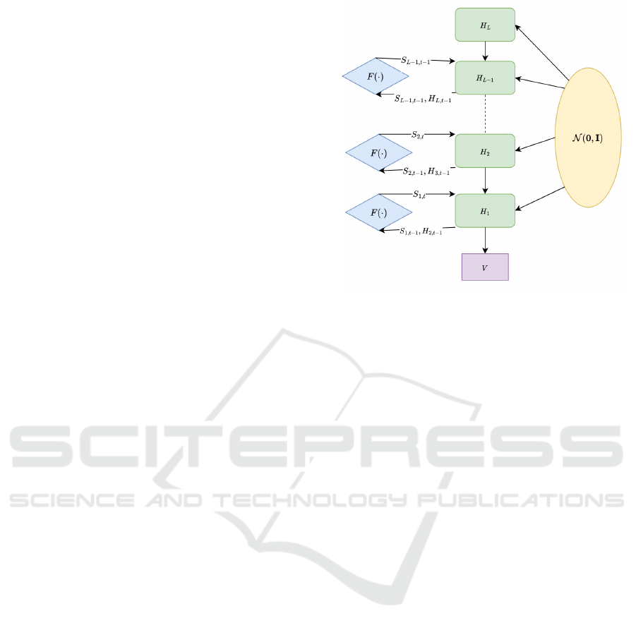
tecture is illustrated in Figure 1. Where the generator
is structured in terms of layers denoted by H. Val-
ues created by the topmost layer (H
L
) are passed to
the one below. The following layer, denoted by H
L−1
,
generates a new value by utilizing a state variable, de-
fined as S
L−1,t−1
and a sample from the Gaussian dis-
tribution N (0, I).
The mean of this Gaussian is the zero vector, while
the covariance is the identity matrix. This process is
repeated until the last layer, where the value v is ex-
tracted. Each layer (except for H
L
) has an additional
function called F, which is the state transition func-
tion. It updates the state value on every layer after
generation.
The generator utilizes a RNN on each layer, asso-
ciated with the “latent temporal states”. We abstrac-
tize them into one single “state” where s
t
denotes the
t
th
vector of relevant temporal information. The state
can also be divided into its corresponding layers. We
use the notation s
l,t
to denote layer and order in the
generation sequence. For example, s
2,5
is the state at
layer 2 at step 5. We define the t
th
vector of stateless
latent information as ξ
t
. It is now possible to define
the current state as dependent on all previous states.
p(s
T
) = p(s
0
)
T −1
∏
t=1
[p(s
t
|s
1:t−1
,ξ
t
)], (7)
where s
T −m:t−1
= [s
T −m
, . .. s
t−1
] We assume that
the importance of any one state decreases to an upper
limit m beyond which past states and latent variables
ICAART 2025 - 17th International Conference on Agents and Artificial Intelligence
312

have no impact. Hence,
p(s
T
) =
T −1
∏
t=T −m
[p(s
t
|s
T −m:t−1
,ξ
t−1
)]. (8)
Our definition of s
t
and F allows a multitude of
different RNNs to be used. We have chosen to use the
cell state of LSTM as our state space S. This means
that our state recognition model has a non-traditional
way of recognizing states. We give it a series of
inputs, discard the output, and then use the internal
temporal representation (cell state) for our generator
model. The usual method would be to utilize the out-
put of the RNN as the state values. Using the cell state
instead of the LSTM outputs allows us to utilize the
learned temporal information over long horizons. To
the best of our knowledge, this method of using the
cell state instead of the LSTM output is new to litera-
ture.
tDLGMs generator model can now be defined as
ξ
l,t
∼ N (ξ
l
|0,I), l = 1 ,..., L, (9)
h
L,t
= G
L
ξ
L,t
, (10)
h
l,t
= R
l
(h
l+1,t
,s
l,t
) + G
l
ξ
l,t
, l = 1, ..., L − 1,
(11)
s
l,t+1
= F
l
(h
l−1,t
,s
l,t
), l = 1,.. .,L − 1, (12)
v
t
∼ π(v|T
0
(h
1,t
)), (13)
where each of the layers l = 1, ...,L − 1 has its own
RNN defined as R
l
, G
l
is a trainable matrix on each
layer, and F
l
is the previously discussed state transi-
tion functions on each layer. ξ is the latent variables
sampled from the Gaussian with zero vector as the
mean and identity matrix as the covariance. Again,
we use LSTM for our RNNs. The chosen RNN dic-
tates the nature of the states and state transition func-
tion. The state on each layer, denoted by s
l,t
, is, there-
fore, a vector of cell states that allow for the capture
of long-term temporal information.
We will now go through the whole generation pro-
cess. The model starts with a sample ξ
l,t
from a Gaus-
sian with the zero vector as mean and identity matrix
as covariance. It is combined with the matrix G
L
, re-
sulting in H
L
. H
L
is then used in the layer below as
input to the RNN defined as R
L−1
(H
L
,s
L−1,t
). The
sum of R
L−1
and G
L−1
ξ
L−1,t
becomes the output of
that layer, denoted by h
L−1
, which is used in the layer
below h
L−2
. This repeats to the last layer h
1
, which
is then used in Equation (13). The h from the layer
above (h
l+1
) is also combined with s
l,t
to create the
next state as seen in Equation (12). The layered latent
variables provide robustness to the stateful model by
interleaving states and latent variables.
Figure 1: This figure shows how values are generated with
tDLGM. It start at H
L
which calculates its value by sam-
pling from N 0, I). This result is then passed down to H
l−1
,
which utilizes H
L
, the current state, and a sample to cal-
culate its value. This is done until the end, resulting in v
as specified in Equation (13). It is also shown on the left-
hand side how the state is updated by the function F on each
layer.
Recall that VAE-based methods aim to approxi-
mate a posterior when a prior is fixed (Kingma, 2013).
The same issue is present for tDLGM as we need to
know both p(s |v) and p(ξ |v). We have two recog-
nition models for this, one being the state recognition
model defined as k and another for the latent variable
defined as q.
Starting with q, which can utilize a method similar
to that of DLGM, see section 4.1 of (Rezende et al.,
2014). That is, we define a posterior for the latent
variable as
q(ξ|V) =
T
∏
t=1
L
∏
l=1
N (ξ
l,t
|µ
l
(v
t
),C
l
(v
t
)), (14)
where the mean µ and covariance C on each layer are
trainable. We take a more novel approach to the state
recognition model. Recall Equation (12), which is re-
sponsible for creating future states that are, as defined
by Equation (8), dependent on m previous states and
latent variables. If the m previous states and latent
variables were known, then it would be possible to
train the state transition function F directly. However,
since this is not known, we instead have to approxi-
mate the state on each layer
F
l
(s
l,t
,h
l+1:L,t
) ≈
ˆ
F
l
(v
t−m:t
) = s
l,t
(15)
where l is the corresponding layer, see Equation (12).
Although we previously defined F
l
as a function of s
and h in Equation (12), F
l
is also implicitly dependent
Approximate Probabilistic Inference for Time-Series Data: A Robust Latent Gaussian Model with Temporal Awareness
313

on ξ as h is dependent on it. Hence, with a slight
abuse of notation, we say that
F
l
(s
l,t
,h
l+1:L,t
) = F
l
(s
l,t
,ξ
l+1:L,t
), (16)
making the relationship more explicit. It has the addi-
tional benefit of a cleaner-looking loss function with-
out altering the underlying implementation.
We further define F and
ˆ
F, where
F(s
t
,ξ
t
) = [F
1
(s
1,t
,ξ
l+1:L,t
),..., F
L−1
(s
L−1,t
,ξ
L,t
)]
and
ˆ
F(v
t−m:t
) = [
ˆ
F
1
(v
t−m:t
),...,
ˆ
F
L−1
(v
t−m:t
)] From
this point forward, we no longer use the individual
layer. Instead, we use our layer-agnostic definitions.
We can then define the approximation as
k(S |V) =
T
∏
t=1
(s
l,t
|
ˆ
F(v
t−m:t−1
)), (17)
or stated another way
p(s
t
|s
t−m:t−1
,ξ
t−m:t−1
) ≈ k(s
t
|v
t−m:t−1
), (18)
this solution is not yet complete. An issue arises due
to the unknown prior p(s). This means that the usual
VAE method cannot be utilized. We will address this
during the derivation of our loss function.
2.1 Deriving the Loss Function
We are now ready to derive the tDLGM loss function.
Broadly speaking, the goal of tDLGM is to maximize
the likelihood of generating the training data V. Tech-
nically, it is achieved by minimizing the negative log-
likelihood given by
L(V) = −log p(V)
= −log
Z
S
Z
ξ
p(V|ξ,S)p(ξ, S)dξdS,
(19)
The negative log-likelihood loss is an integral over
S×ξ, which is the cross product of the state and latent
variable space.
Both s and ξ have unknown posteriors p(s|v) and
p(ξ|v) which was addressed in the previous section by
introducing two recognition models: the state recog-
nition model k(s|v) ≈ p(s|v) and the latent recog-
nition model q(ξ|v) ≈ p(ξ|v). We, for the sake of
brevity, define k(s)q(ξ) = β(s,ξ). Both recognition
models are included in the loss. Jensen’s inequality is
then used to get a surrogate loss
L(V) = − log
Z
S
Z
ξ
β(s,ξ)
β(s,ξ)
p(V|ξ,S)p(ξ, S)dξdS
≤ −
Z
S
Z
ξ
β(s,ξ)log

p(V|ξ,S)p(ξ, S)
β(s,ξ)

dξdS,
(20)
the properties of the logarithm and the fact that the
integral of a probability density function is equal to
one leaves us with
L(v) ≤ D
KL
(k(S)||p(S)) + D
KL
(q(ξ)||p(ξ))−
E
q(ξ),k(S)
[log(p(V|S,ξ))].
(21)
Recall the definition of the posterior in Equation
(14). We use this to say that
D
KL
(q(ξ)||p(ξ)) = D
KL
(N (µ,C)||N (0,1)). (22)
which we will solve analytically.
The probability for k has been previously defined
as
p(s
t
|s
t−m:t−1
,ξ
t−m:t−1
) ≈ k(s
t
|v
t−m:t−1
), (23)
state, latent variables, and how they influence the cur-
rent state is approximated based on true values v. It
is then possible to use an approximated state for the
generation of future states
p(s
t+1
|F(s
t−m:t
,ξ
t−m:t
)) ≈
p(s
t+1
|F(
ˆ
F(v
t−m:t−1
),ξ
t
)),
(24)
meaning that we use
ˆ
F to approximate an intermedi-
ate state s
t
. This intermediate state is then used by the
generator model to generate the next state s
t+1
. This
is useful as it allows us to generate an approximate
state through two methods. The first method uses the
approximation function
ˆ
F. While the second method
receives an approximation from
ˆ
F, which is then used
in the true state transition function F. Applying this
to the KL divergence results in
D
KL
(k(S)||p(S)) = D
KL
(k(S
t+1
)||p(S
t+1
))
≈ D
KL
(k(S
t+1
)||p(F(k(S
t
|V
t−m:t
),ξ
t
)).
(25)
Our final issue arises because it is difficult to calcu-
late the above KL-divergence. This is the case be-
cause both F and
ˆ
F are deterministic functions, and
the prior p(s) is unknown. We addressed this by cal-
culating the Mean Squared Error (MSE)
D
KL
(k(S)||p(S)) ≃ αMSE(
ˆ
F(V
t+1
),F(
ˆ
F(V
t
),ξ
t
)),
(26)
where α is added as a scaling factor to account for
the fact that the KL-divergence and MSE are differ-
ent metrics. To summarize, we approximate s
t
with
function
ˆ
F(v
t−m:t−1
) = s
t
. Our approximation is then
used to generate s
t+1
, F(
ˆ
F(v
t−m:t−1
),ξ
t
) = s
t+1
. This
generated state is then compared against an approxi-
mated state through MSE(
ˆ
F(v
t
),F(
ˆ
F(v
t−1
,h
t
))). Re-
call that we are comparing the cell state as created by
the state recognition model and the generator model.
Minimizing the MSE means that we train the state
recognition model and generator model to
ICAART 2025 - 17th International Conference on Agents and Artificial Intelligence
314

Another alternative is to predict the distribution of
the next state with our state recognition model. The
KL-divergence can then be approximated as a log-
likelihood instead of MSE.
Equations (22) and (26) can then be applied in the
surrogate loss
L(V) ≤ D
KL
(k(S)||p(S)) + D
KL
(q(ξ)||p(ξ))
− E
q(ξ),k(S)
[log(p(V|s,ξ))]
≈ D
KL
(N (µ,C))||N (0,I))
+ αMSE(F(V
t+1
),F(
ˆ
F(V
t
),h(ξ
t
)
− E
q(ξ),k(S)
[log(p(V|s,ξ))],
(27)
where the KL-divergence can be calculated analyti-
cally, resulting in the final loss
1
2
∑
l,n
[||µ
n,l
||
2
+ Tr(C
n,l
) − log |C
n,l
| − 1]
+ α MSE(k(S
S
S
+
), p(S
S
S
+
))
− E
q(ξ
ξ
ξ),k(s
s
s)
[log((p(v
v
v|s
s
s,ξ
ξ
ξ,θ)p(θ))].
(28)
3 EXPERIMENTS
1
Our experiments were performed with a dataset pro-
vided by Alibaba under a free license for research use
(Weng et al., 2023). It is a tabular dataset containing
traces of different data center tasks with their times-
tamps, resource requirements, etc. We are interested
in the column associated with the GPU requirements -
titled GPU MILLI. Also note that the arrival, deletion,
and schedule times are discarded. In other words, we
are only interested in predicting the next GPU require-
ment not when it arrives.
tDLGM is compared to two baseline models. Our
first baseline model is a traditional RNN consisting
of LSTM units (Hochreiter and Schmidhuber, 1997).
While DLGM is used as the second baseline model
(Rezende et al., 2014). DLGM, as previously dis-
cussed, is stateless and therefore the vanilla version
cannot be used for time-series prediction tDLGM. In
order to still use it as a baseline, we provide as input
a fixed length vector of historical data for the next-
step prediction. Thereby explicitly providing tempo-
ral data relations within the history that is provided as
input DLGM. With this modification, we still expect
poor performance since the dataset has very long-term
temporal connections between data points that will
probably be missed by the provided historical vector.
It is worth noting that the historical vector is only pro-
vided as input during training and not during the data
generation stage.
1
The code for tDLGM can be found here:
https://git.cs.kau.se/johaanto/tdlgm
As mentioned in the Abstract and Introduction, we
are interested in robust Generative AI models. Models
such as RNN and DLGM are not known to be robust.
Here, robustness is achieved by adding low variance
Gaussian noise to the training data in the hope that
this would simulate any real-world noise that is en-
countered during prediction (testing phase). For ex-
ample, the authors of DLGM found that it could only
reconstruct effectively when noise was artificially in-
jected into the training dataset (Rezende et al., 2014).
On the other hand, we train tDLGM on the given unal-
tered dataset. We test its efficacy with respect to both
reconstruction and data generation using noisy test
data. In short, it beats the baselines. Further, there
was no statistically significant performance degrada-
tion due to the presence of noise in the testing phase
that was absent during the training phase. Through
this, we concluded that tDLGM is robust to additive
Gaussian noise.
Generally speaking, a time-series predictor is ei-
ther used for data imputation or for lookahead pur-
poses (predict the future). A good predictor must
predict reliably over longer time horizons. In recent
years, robustness to data errors has also become a
desirable property. Hence, we compare tDLGM to
the baselines with respect to imputation performance,
prediction error as a function of the prediction hori-
zon, and with respect to robustness to data errors. Be-
low, we describe them in further detail.
1. Imputation, where we feed noisy data (additive
Gaussian noise) into our models and see how well
they reconstruct the true data. The imputation
is performed on test data that was not used dur-
ing training. As the dataset is simple, and since
we explicitly feed DLGM with temporal infor-
mation, we expect it to perform well. We ob-
served that DLGM has the lowest MSE capable
of reconstructing close to perfectly, followed by
tDLGM. However, we argue that the lower MSE
and variance of DLGM do not mean it is better
than tDLGM. This will be discussed in the Re-
sults section.
RNN, on the other hand, has significantly worse
performance, as illustrated in Figure 2. We re-
peated the experiments with varying levels of
added Gaussian noise.
2. Multiple time-step prediction, where we require
the models to predict over multiple time-steps in
the future. This set of experiments is important
since it is known that prediction errors typically
accumulate over time when predicting over mul-
tiple steps. This is because predicted values are
themselves used to predict more values that are
further into the future. We may consider two met-
Approximate Probabilistic Inference for Time-Series Data: A Robust Latent Gaussian Model with Temporal Awareness
315

rics: the average mean squared error over the pre-
diction horizon and the similarity of the generated
values to the true distribution. We use the lat-
ter since we are interested in the model’s ability
to capture trends in the given time-series dataset.
We are not interested in exactly duplicating the
dataset. Standard metrics such as MSE score how
well a generative model can predict given data
points. One of our future goals is to use this gen-
erative model in cases where the data is limited.
If it were to recreate the already limited dataset
accurately, it would lose its purpose. We want
it to generate new but similar data, not the same
data. The used metric is explained in Algorithm
1. tDLGM performed best, followed by DLGM
and then RNN.
3. Robustness, where we check by how much the
model performances degrade due to errors in the
dataset. One core idea of tDLGM is that inter-
leaving state and latent variables should facilitate
robust prediction. That is, the generative model
should still be able to perform given uncertainties
in data. One previously discussed method of in-
creasing robustness is to train a model on noisy
data. DLGM, for example, struggled with recog-
nition of unseen data without this (Rezende et al.,
2014). Therefore, we want tDLGM to reconstruct
unseen data without training it on noisy data. Our
tests prove that tDLGM can reconstruct without
training on noisy data, validating the claim that
tDLGM is robust.
As mentioned before, adding Gaussian noise to
the training dataset is one way Machine Learning en-
gineers hope to achieve robustness. In some cases,
artificially injecting errors into the dataset can be a
requirement for good learning (Rezende et al., 2014).
However, what happens if we train for one kind of er-
ror but encounter errors of another type during test-
ing? For example, mean zero low variance Gaus-
sian noise is typically added to training data for this
purpose. What if we encounter biased noise during
testing? Hence, the artificial noise injected must be
problem-specific. Learning models such as ours ex-
hibit robustness properties and are better equipped to
handle such problematic scenarios.
4 RESULTS
Since the data was not very complex (limited long-
term temporal dependencies), and since we explicitly
provided a vector of past history as input to DLGM, it
performed well when it came to data reconstruction.
Data: T ← true data
Data: G ← generated data
Data: s ← step forward in time
Data: T M ← matrix initialized to zero
Data: GM ← matrix initialized to zero
for t
i
∈ T, ∀t
i
,where t
i+s
∈ T do
T M
t
i
,t
i+s
← T M
t
i
,t
i+s
+ 1
end
for g
i
∈ G,∀t
i
,where g
i+s
∈ G do
GM
g
i
,g
i+s
← GM
g
i
,g
i+s
+ 1
end
GM ←
|T |
/|G| × GM Scale values in GM
based on amount of data points.
score =
∑
i
∑
j
min(GM
i, j
,T M
i, j
)
/T M
i, j
,∀i, j T M
i, j
̸= 0
Algorithm 1: Evaluation of future prediction. Models are
scored by grouping their generated values into intervals.
The algorithm then counts how many instances of a specific
value are generated after another value. Therefore, distri-
butions are formed over what values are usually generated
when. The overlap between the true and generated distri-
butions is then used as the score. It assumes that T and
G contain a finite set of values corresponding to intervals,
or so-called buckets of values. Scaling is also performed,
accounting for the fact that T and G might have different
amounts of values.
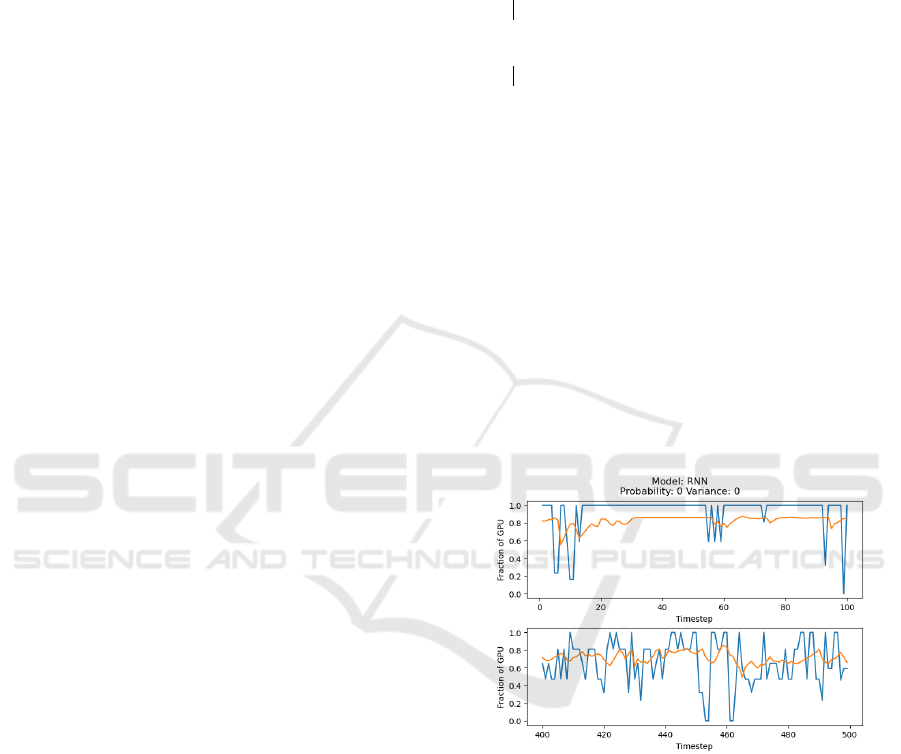
Figure 2: The best performing RNN model for reconstruc-
tion when using a naive MSE scoring method. Blue are the
true values and orange is the generated values. The Y-axis
specifies what fraction of a GPU a task at a specific step
requires, with a maximum of 1 and minimum of 0. It is ev-
ident that the reconstruction process performs poorly.
With tDLGM as a close second, the basic RNN
performed worst out of all the models. See Table 1 for
a complete table of the different values that were tried
and their mean squared error. Here, it is evident that
DLGM was almost unaffected by the noise, generat-
ing accurate values with close to the same variance
for all cases. RNN is also unaffected. This is because
noise was added to the training data before training
the DLGM and RNN models - a standard practice to
ICAART 2025 - 17th International Conference on Agents and Artificial Intelligence
316

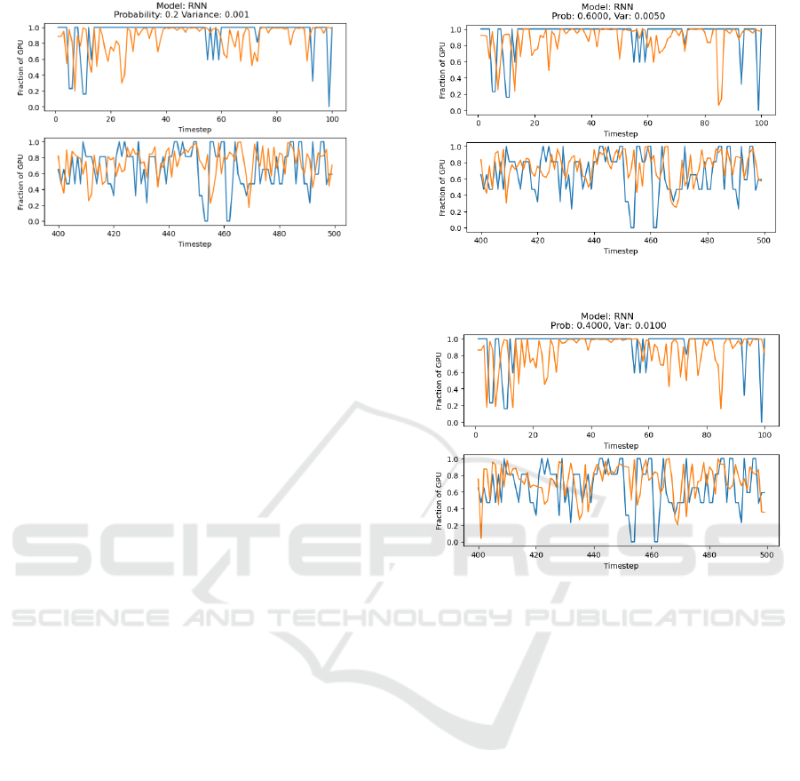
Figure 3: A model that performed worse than the best per-
forming RNN when using a naive MSE scoring method.
Blue represents true values, and orange represents the gen-
erated values. The Y-axis specifies what fraction of a GPU
a task at a specific step requires, with a max of 1 and a
minimum of 0. The probability and variance denote the in-
troduction of error. With the probability denoting the like-
lihood of modifying a value and the variance specifying the
magnitude of change according to a Gaussian.
improve the robustness of models that are not inher-
ently robust. Figure 2 shows a slice of the best re-
construction, while figure 3 shows the worst slice (ac-
cording to the mean squared error metric). From a vi-
sual inspection, it appears that the worser model fol-
lows the pattern while the better scoring model does
not. Therefore, a filtering process is performed in the
form of a t-test. It looks at the changes in the recon-
structed data given different levels of additive noise.
This filtering assumes that the reconstruction is neg-
atively affected to such a degree that it is statistically
significant. All trained instances with a p-value above
0.7 were excluded, leaving us with the new values we
call Filtered RNN in Table 1. The high p-value is set
to counteract the risk of confirmation bias. We as-
sume that the error increases with the noise but do not
want to filter out evidence proving the contrary.
Our new results make it evident that RNN is much
more sensitive to noise as compared to both tDLGM
and DLGM. Hence, we conclude that tDLGM per-
forms better than the regular RNN at value imputa-
tion. Figures 7, 8, and 9 show the reconstruction
without any noise for tDLGM, DLGM, and RNN re-
spectively. Reconstruction with noise can be seen in
Figures 4, 6, and 5. DLGM’s ability to perfectly re-
construct should not be interpreted as it being a bet-
ter model as compared to tDLGM. The simplicity of
the data means that DLGM can easily overfit. Be-
sides, perfect reconstruction is an indication that the
model does not generalize well. It is better to have
a reconstruction model - such as tDLGM - that gen-
erates similar values, but not exact values. This is
also an indication of the robustness of tDLGM. Fur-
(a) Probability of modifying value: 60%, modifying
through a Gaussian with variance set to 0.005.
(b) Probability of modifying value: 40%, modifying
through a Gaussian with variance set to 0.01.
Figure 4: RNN tasked with reconstructing the test dataset.
The orange line is generated values, and the blue is true val-
ues. The X-axis is time. The Y-axis specifies what fraction
of a GPU a task requires at a specific step, with a maximum
of 1 and a minimum of 0.
ther research must be conducted with higher dimen-
sional and more complex time-series data, to see how
this changes performance.
In order to evaluate the data generation capability,
we score based on the multiple-time-step prediction
distributions - check if they match the empirical fu-
ture distributions estimated from the dataset. We do
not compare the values themselves, e.g., using mean-
squared error. We are interested in the distribution of
future values not the actual values themselves. Al-
gorithm 1 describes this metric. Scoring is done on
a dataset of future generations. It was generated by
giving each model a sequence of values, which was
then used to create future values see Table 2 for re-
sults. RNN performs well for shorter prediction hori-
zons. However, it quickly deteriorates when gener-
ating longer sequences. tDLGM is stable with close
to the same score no matter how long the prediction
Approximate Probabilistic Inference for Time-Series Data: A Robust Latent Gaussian Model with Temporal Awareness
317

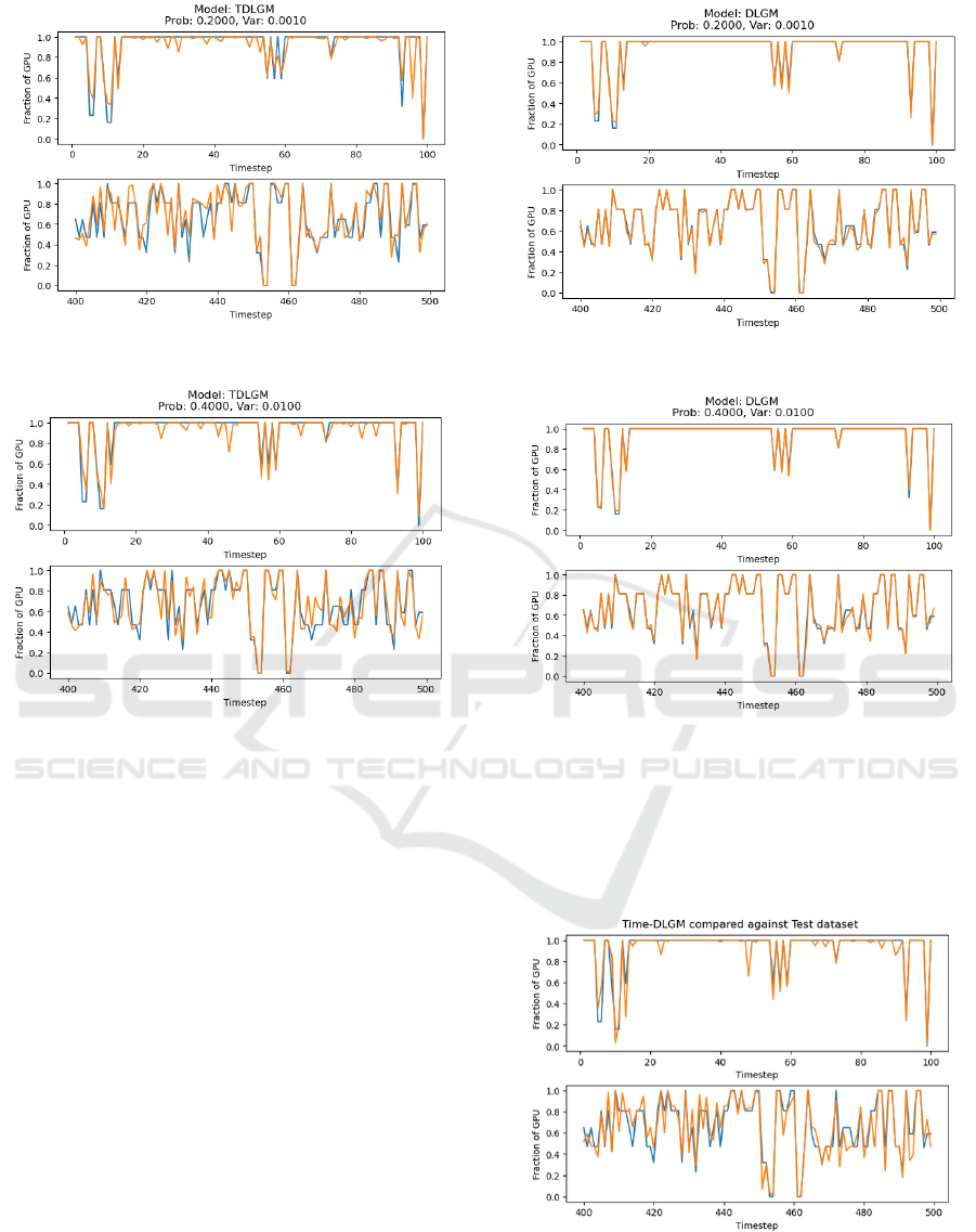
(a) Probability of modifying value: 20%, modifying
through a Gaussian with variance set to 0.001.
(b) Probability of modifying value: 40%, modifying
through a Gaussian with variance set to 0.01.
Figure 5: tDLGM tasked with reconstructing the test
dataset. The orange line is generated values, and the blue
is true values. The X-axis is time. The Y-axis specifies
what fraction of a GPU a task requires at a specific step,
with a maximum of 1 and a minimum of 0. Subfigures 5a
and 5b show the model’s performance with different noise
levels added.
horizon is set to. DLGM also exhibit this stable be-
havior but with a lower score than tDLGM. From this,
we conclude that tDLGM provides a more consistent
data generation as compared to RNN and DLGM.
We will now discuss the robustness of tDLGM.
Models are usually trained by combining true values
with artificial noise, a common practice to improve
robustness. If tDLGM exhibits robustness properties,
then this should not be required. We evaluated this
by training tDLGM with the unmodified training data
and then performed reconstructions (imputation). Re-
constructions were, as before, performed with varying
magnitudes of noise. Our results can be seen in Table
3. Here, it is evident that the reconstruction performed
more or less similarly without the added noise. Al-
though it was still significantly better than that of
RNN, which can be seen in Table 1. We conclude
(a) Probability of modifying value: 20%, modifying
through a Gaussian with variance set to 0.001.
(b) Probability of modifying value: 40%, modifying
through a Gaussian with variance set to 0.01.
Figure 6: DLGM tasked with reconstructing the test dataset.
The orange line is generated values, and the blue is true val-
ues. The X-axis is time. The Y-axis specifies what fraction
of a GPU a task requires at a specific step, with a maximum
of 1 and a minimum of 0. Subfigures 6a and 6b show the
model’s performance with different noise levels added.
Figure 7: tDLGM tasked with reconstructing the test
dataset. Orange is generated values and blue is true values.
The X-axis is time. The Y-axis specifies what fraction of a
GPU a task at a specific step requires with a max of 1 and 0
as minimum. It is evident from the figure that tDLGM can
reconstruct the data.
ICAART 2025 - 17th International Conference on Agents and Artificial Intelligence
318

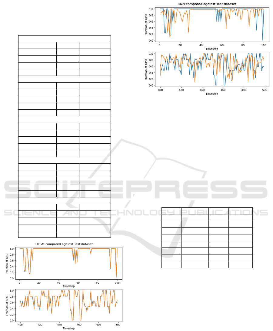
Table 1: Table showing how well the different models re-
constructed the test data. Each data point had a percentual
chance of being modified through a Gaussian sample. The
variance was modified to see how each model reacted to
different magnitudes of error.
Probability: 0, Variance: 0
Model MSE Variance
tDLGM 0.0122 0.0083
DLGM 0.0006 7.0 × 10
−6
RNN 0.0773 0.0164
Filtered RNN 0.1038 0.0329
Probability: 0.2, Variance: 0.001
Model MSE Variance
tDLGM 0.0122 0.0009
DLGM 0.0006 4.9 × 10
−6
RNN 0.0773 0.0164
Filtered RNN 0.0794 0.0153
Probability: 0.6, Variance: 0.005
Model MSE Variance
tDLGM 0.0118 0.0124
DLGM 0.0006 4.8 × 10
−6
RNN 0.0773 0.0164
Filtered RNN 0.1033 0.0323
Probability: 0.4, Variance: 0.01
Model MSE Variance
tDLGM 0.0114 0.0014
DLGM 0.0006 4.4 × 10
−6
RNN 0.0773 0.0164
Filtered RNN 0.0827 0.0172
Probability: 0.8, Variance: 0.05
Model MSE Variance
tDLGM 0.0118 0.0008
DLGM 0.0007 6.8 × 10
−6
RNN 0.0773 0.0164
Filtered RNN 0.0788 0.0153
Figure 8: DLGM compared against the test dataset. Or-
ange is the generated values, and blue is the true values.
The X-axis is the steps in an unspecified time unit, where
one generation is performed each step. The Y-axis speci-
fies what fraction of a GPU a task at a specific step requires
with a max of 1 and 0 as minimum. DLGM can perfectly
reconstruct values in many instances, as evident by the high
overlap.
Figure 9: RNN tasked with reconstructing the test dataset.
Orange is generated values and blue is true values. The X-
axis is time. The Y-axis specifies what fraction of a GPU a
task at a specific step requires with a max of 1 and 0 as mini-
mum. It is evident from the figure that RNN can reconstruct
data, although much worse than the other two models.
Table 2: Table showing how well the different models gen-
erated future values. A higher score correlates with a larger
overlap between the true and generated values. Scoring is
done with Algorithm 1. Steps defines the number of con-
secutive digits generated for each test. For example, a se-
quence length of 30 means that a state was fed, which was
then used to create the following 30 values. We can con-
clude from this that tDLGM was best at generating future
values that look similar to the actual distribution, followed
by DLGM and then RNN.
Steps tDLGM RNN DLGM
2 62.47 58.48 59.87
5 63.47 58.48 59.67
8 63.21 58.41 60.32
10 63.59 58.04 59.67
15 63.67 57.79 60.11
20 63.54 58.01 60.36
25 63.31 57.80 59.89
30 63.31 58.01 60.33
based on this that tDLGM is inherently robust and can
generalize better to values outside of the training set
without the need for any standard robustness-inducing
techniques. Figures 10 show the reconstruction for
two types of additive noise.
5 CONCLUSION
We have proposed a new model called tDLGM, based
on the ideas of a recognition-generator structure with
state. tDLGM differ from other models commonly
seen in the literature by using two recognition models,
one for state and one for latent variables. Both state
and latent variables are combined in an interleaving
Approximate Probabilistic Inference for Time-Series Data: A Robust Latent Gaussian Model with Temporal Awareness
319

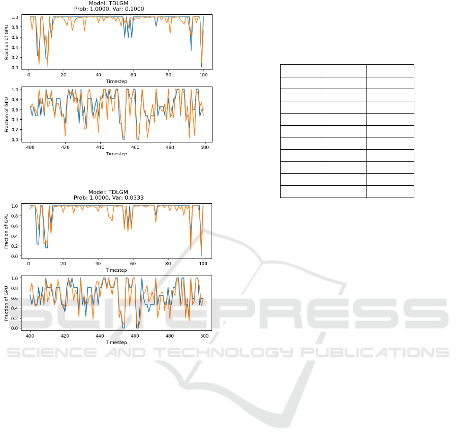
(a) Probability of modifying value: 100%, modifying
through a Gaussian with variance set to 0.1.
(b) Probability of modifying value: 100%, modifying
through a Gaussian with variance set to 0.0333.
Figure 10: tDLGM tasked with reconstructing the test
dataset. The orange line is generated values, and the blue
is true values. The X-axis is time. The Y-axis specifies
what fraction of a GPU a task requires at a specific step,
with a maximum of 1 and a minimum of 0. Subfigures 10a
and 10b show the model’s performance with different noise
levels added
structure, which allows for the learning of complex
temporal relations. Furthermore, to our knowledge,
the state recognition model and the regularization we
derive from it are a novel inference method. Our ex-
periments on the Alibaba trace dataset (Weng et al.,
2023) show that tDLGM is a promising model with
good performance with regard to imputation, the gen-
eration of new values, and robustness. We, through
this, showed that tDLGM is a generative model suit-
able for modeling long-term temporal relationships.
However, there are also some points for future
improvements. Due to the inherent complexity of
tDLGM, we expect that it requires more data to train
when compared to DLGM, which has a simpler archi-
tecture. Additionally, we did not spend an inordinate
Table 3: Table showing how well tDLGM managed to
reconstruct unseen values based on different amounts of
noise. Each data point in the test dataset was modified
according to the Gaussian N (0,σ
2
) where σ
2
is varied
variance. The output was clamped to the range [0, 1].
tDLGM was trained purely on the unmodified training data.
σ
2
MSE Variance
0.0053 0.01306 0.00090
0.0059 0.01371 0.00099
0.0067 0.01214 0.00080
0.0077 0.01221 0.00079
0.0091 0.01275 0.00088
0.0111 0.01288 0.00086
0.0143 0.01287 0.00089
0.0200 0.01328 0.00095
0.0333 0.01315 0.00081
0.100 0.01938 0.00168
amount of time on hyperparameter optimization, in-
stead opting for a simple grid search method. This
was done because the ease of implementation was
one of our goals. Hence, we experienced that training
runs needed to be restarted with a probability of .25.
We conjecture that this is due to the aforementioned
complexity, the smaller dataset, and the need to ex-
tract temporal information. For more complex prob-
lems, we expect that more thorough hyperparameter
optimization will be required in addition to a larger
dataset.
Another avenue of future research is to make a
more exhaustive comparison against other models for
time-series data, such as VRNN (Chung et al., 2015).
It would also be interesting to explore the approxima-
tion from Equation (26) in further detail.
REFERENCES
Chung, J., Gulcehre, C., Cho, K., and Bengio, Y. (2014).
Empirical evaluation of gated recurrent neural net-
works on sequence modeling.
Chung, J., Kastner, K., Dinh, L., Goel, K., Courville, A. C.,
and Bengio, Y. (2015). A recurrent latent variable
model for sequential data. CoRR, abs/1506.02216.
Hochreiter, S. and Schmidhuber, J. (1997). Long Short-
Term Memory. Neural Computation, 9(8):1735–1780.
Johansson, A. (2024). Generative ai for time dependent
data. Master’s thesis, Karlstad University, Department
of Mathematics and Computer Science (from 2013).
Karras, T., Aila, T., Laine, S., and Lehtinen, J. (2017). Pro-
gressive growing of gans for improved quality, stabil-
ity, and variation. arXiv preprint arXiv:1710.10196.
Kingma, D. P. (2013). Auto-encoding variational bayes.
arXiv preprint arXiv:1312.6114.
Mehmeti, F. and Porta, T. F. L. (2021). Analyzing a 5g
dataset and modeling metrics of interest. In 2021
ICAART 2025 - 17th International Conference on Agents and Artificial Intelligence
320

17th International Conference on Mobility, Sensing
and Networking (MSN), pages 81–88.
Rezende, D. J., Mohamed, S., and Wierstra, D. (2014).
Stochastic backpropagation and approximate infer-
ence in deep generative models. In International
conference on machine learning, pages 1278–1286.
PMLR.
Weng, Q., Yang, L., Yu, Y., Wang, W., Tang, X., Yang,
G., and Zhang, L. (2023). Beware of fragmentation:
Scheduling gpu-sharing workloads with fragmenta-
tion gradient descent. In 2023 USENIX Annual Tech-
nical Conference, USENIX ATC ’23. USENIX Asso-
ciation.
Yin, H. and Berger, C. (2017). When to use what data set for
your self-driving car algorithm: An overview of pub-
licly available driving datasets. In 2017 IEEE 20th In-
ternational Conference on Intelligent Transportation
Systems (ITSC), pages 1–8.
Yoon, J., Jarrett, D., and Van der Schaar, M. (2019). Time-
series generative adversarial networks. Advances in
neural information processing systems, 32.
Approximate Probabilistic Inference for Time-Series Data: A Robust Latent Gaussian Model with Temporal Awareness
321