A Framework for Developing Robust Machine Learning Models in

Harsh Environments: A Review of CNN Design Choices

William Dennis

and James Pope

Communication Systems and Networks Group, University of Bristol, Bristol, U.K.

Keywords:

Robust Machine Learning, Fault Tolerance, Harsh Environments, Convolutional Neural Network, Single

Event Effects, Activation Functions, Dropout, Regularisation, Pooling.

Abstract:

Machine Learning algorithms are envisioned to be used in harsh and/or safety critical environments such as

self-driving cars, aerospace, and nuclear sites where the effects of radiation can cause errors in electronics

known as Single Event Effects (SEEs). The effect of SEEs on machine learning models, such as neural net-

works composed of millions of parameters, is currently unknown. Understanding the models in terms of

robustness and reliability is essential for their use in these environments. To facilitate this understanding, we

propose a novel framework to simulate SEEs during model training and inference. Using the framework we

investigate the robustness of the Convolutional Neural Network (CNN) architecture with dropout, regularisa-

tion and activation functions under different error models. Two new activation functions are suggested that

decrease error by up to 40% compared to ReLU. We also investigate an alternative pooling layer that can

provide model robustness with a 16% decrease in error with ReLU. Overall, our results conﬁrm the efﬁcacy

of the framework for evaluating model robustness in harsh environments.

1 INTRODUCTION

The advent of Neural Network architectures

has shifted the paradigm from traditional, well-

understood image processing methods towards more

complex, less-understood models. This black-box

nature of state-of-the-art models can pose unforeseen

dangers when applied to industry and exposed to

Single Event Effects (SEEs). Therefore The focus

of this research is to directly attack the black-box of

these complex models via simulated SEEs.

SEEs are radiation induced errors on electronic

devices that could result in changes to the software

running. For use in safety-critical environments, such

as driverless systems, understanding how a Machine

Learning (ML) model behaves under SEEs is impera-

tive. Many example situations and further motivation

are outlined in Chapter 2. Robustness in ML systems

are therefore a key requirement that has typically been

referred to as the performance of a model under at-

tacks to the input data. On the other hand, attacks

to the parameter space in ML models are far less ex-

plored and do not ﬁt under the adversarial robustness

umbrella.

https://orcid.org/0009-0005-4769-3136

https://orcid.org/0000-0003-2656-363X

Convolutional Neural Networks (CNNs) are a

common ML model aimed to solve image process-

ing tasks. First introduced in 2012, CNNs have

consistently been the highest performing architecture

across image classiﬁcation competitions, such as the

ImageNet Large Scale Visual Recognition Challenge

(Krizhevsky et al., 2012). This 2012 CNN model

was called AlexNet and is an example of a Deep

Neural Network (DNN) consisting of over 60 mil-

lion parameters across 5 convolutional layers and 3

fully connected layers. The power of these models

derives from their ability to learn hierarchical repre-

sentations of data with every layer abstracting features

from the raw inputs. Therefore it is unsurprising the

improvements over AlexNet have come with an in-

creased number of layers. DNNs, with their many

layers and huge parameter space, further exemplify

the black box narrative.

There is limited research on perturbations to the

weights and biases of the CNN architecture, which

can be a result of SEEs. Research on SEEs is an

extremely challenging area as the natural phenomena

occurs at a very low probability, making experimen-

tation very hard. Facilities, such as ChipIr can arti-

ﬁcially generate SEE-like particles to perform beam

experiments. This experimentation can produce more

322

Dennis, W. and Pope, J.

A Framework for Developing Robust Machine Learning Models in Harsh Environments: A Review of CNN Design Choices.

DOI: 10.5220/0013155000003890

Paper published under CC license (CC BY-NC-ND 4.0)

In Proceedings of the 17th International Conference on Agents and Artiﬁcial Intelligence (ICAART 2025) - Volume 2, pages 322-333

ISBN: 978-989-758-737-5; ISSN: 2184-433X

than 30 million years of natural irradiation in 241

hours (Rech Junior et al., 2022). Although this speeds

up the natural process exponentially, experimentation

is limited by the availability of these devices. Alter-

native approaches have looked towards fault injection

software to simulate SEEs (Hari et al., 2017) but there

is no standardised solution. These beam-experiments

also focus on the sensitivity of hardware, and there-

fore suggest hardware solutions, with minimal regard

to high-level radiation hardening techniques.

This research aims to start addressing this gap by

exploring how CNN design choices inﬂuence the ro-

bustness to SEEs. A number of CNN models are built

in the Pytorch deep learning framework and trained

on an example scenario/dataset. Informed by existing

research, an error model simulating SEEs was built

to test these CNNs. Finally a comprehensive analy-

sis of the results from these tests was performed. The

contributions of the paper are as follows:

• Novel framework for evaluating neural networks

in harsh environments

• Propose two novel activation functions that are

shown to be more robust to SEE related errors.

• Propose novel pooling layer that is also shown to

be more robust to SEE related errors.

2 TECHNICAL BACKGROUND

2.1 History of SEEs and Motivation

SEEs have been known to disrupt spacecraft from the

1970s, and as early as 1962 the idea of SEEs were

ﬁrst suggested (Wallmark and Marcus, 1962). Binder,

Smith and Holman produced foundational work with

their 1975 paper “Satellite Anomalies from Galactic

Cosmic Rays” (Binder et al., 1975). Here, the authors

were the ﬁrst to report SEEs in operating satellites

and explored the mechanisms by which cosmic rays

impact microelectronics that have resulted in satellite

communication anomalies. Spacecraft are one exam-

ple of the many harsh environments impacted by the

effects of SEEs and it is clear that the mitigation tech-

niques are essential to enabling the use of electronics

in these environments.

Another area of concern are safety-critical envi-

ronments as SEEs have been shown to occur in every-

day environments. A harmless example popularised

by the media was a Mario speedrunning tournament

where player was aided by a bit change (bitﬂip) in

Source code is available at https://github.com/wd7512/

MSc-Thesis-2024/

the memory of the computer running the game. A

more disastrous case was in 2008, during the ﬂight of

an Airbus A330 between Singapore and Perth. SEEs

sadly resulted in 12 serious injuries when the A330

started nose-diving on two separate occasions (Bu-

reau, 2008)

The miniaturisation of electronics is another fac-

tor driving the need for SEE mitigation techniques.

Transistors, explained in more detail later, are the ba-

sic building block of electronics and have increas-

ing sensitivity to SEEs as miniaturisation progresses.

Moore’s law states that the number of transistors on

an integrated circuit doubles approximately every two

years (Moore, 1998). This has generally held true

since the idea in 1965 with the modern day 3nm

process transistors being less than 50nm in length

(Badaroglu, 2021). The sensitivity arises from the

critical charge required to change the state of the tran-

sistor being proportional to the size. Therefore as

electronic devices become more powerful with more

transistors, smaller transistors and higher transistor

density, ionizing radiation requires less energy to in-

duce an SEE. Consequently, the number of SEEs are

set to increase.

2.2 SEEs and Transistors

Edward Peterson deﬁnes SEEs as the action of a sin-

gle ionizing particle as it penetrates sensitive nodes

within electronic devices. SEEs in space arise from

two natural sources, heavy ions from cosmic rays or

solar ﬂares and protons trapped in the earths magnetic

ﬁeld. An ion is an atom or molecule with a net pos-

itive or negative charge. This is a result of an imbal-

ance between the number of electrons, that hold nega-

tive charge, and number of protons, that hold positive

charge. Many devices can be upset by these ions at a

rate of about 10

−6

upsets per bit each day (Peterson,

2011).

Named after Van Allen’s discovery in 1958,

the Van Allen radiation belts are zones of ener-

getic charged particles originating from solar winds

and held in place by the earths magnetic ﬁeld

(VAN ALLEN et al., 1958). There is an inner and

outer region which can be dangerous for satellites to

operate in. Peterson states that individual protons can

be found here but have an energy level too low to up-

set most devices via direct ionisation. However, one

proton in 10

will undergo a nuclear reaction within

the body of a transistor capable of an upset. There-

fore, at the heart of the belt, 1KB of memory would

have 10 upsets a day, a dangerously high number (Pe-

terson, 2011).

The transistor is the most fundamental building

A Framework for Developing Robust Machine Learning Models in Harsh Environments: A Review of CNN Design Choices

323

Heavy Ion

High Energy Proton

Heavy Ion

Reaction

Track of Ions

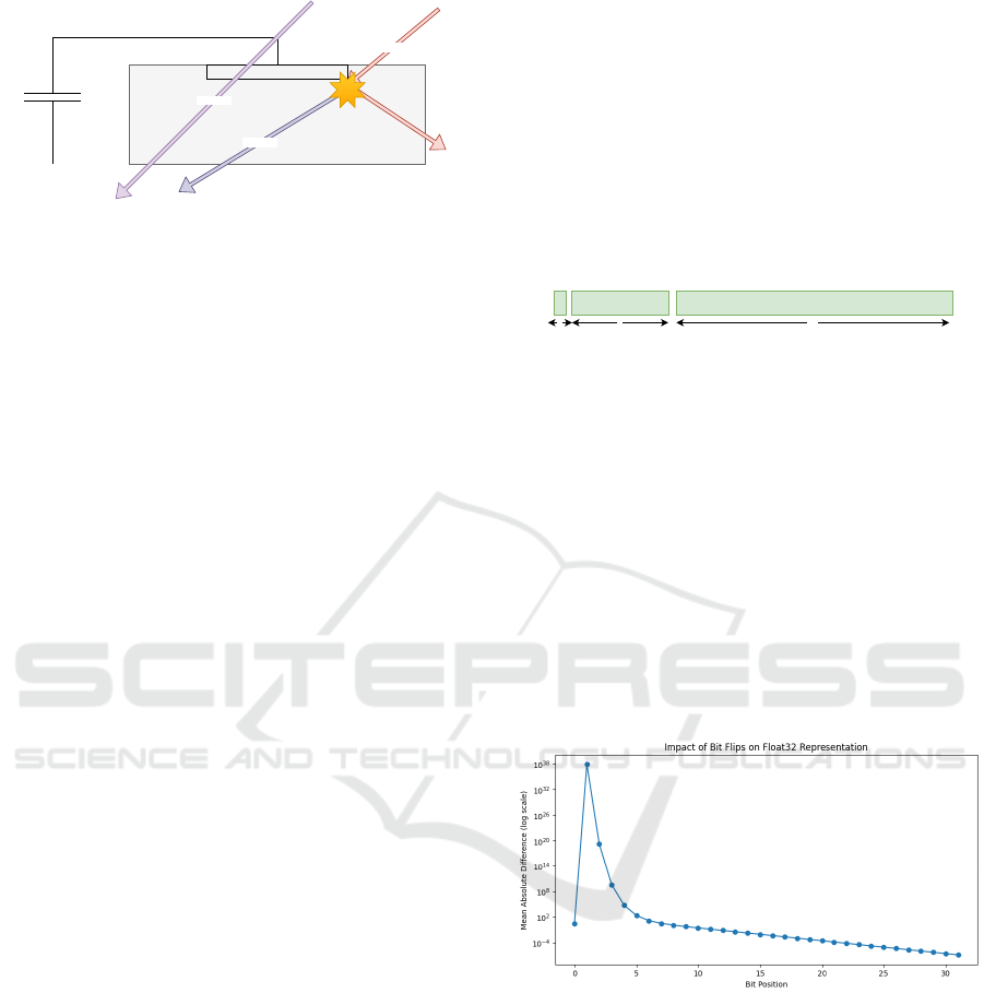
Figure 1: Ionisation paths though a transistor that can dis-

rupt the state.

block of all modern day electronics. It is a type of

semiconductor used to switch or amplify electric sig-

nals and power. Combining transistors together allow

for the storage of information and the execution of

complex logic operations, forming the basis of mem-

ory cells, processors, and virtually all digital elec-

tronic devices.

Peterson states that a heavy ion can deposit a track

of ions as it passes through the body of the transistor

shown in Figure 1. This produces an electric pulse or

signal that may appear valid to the device, changing

the state of the transistor. Protons passing through the

body of the transistor have no immediate effect but

can cause a nuclear reaction in the silicon. This can

produce heavy ions that achieve the same effect.

Peterson divides SEEs into eight subcategories,

but the focus are on Single Event Upsets (SEUs) and

Multi-Bit Upsets (MBU). Both involve changes to

computer memory via the change of a bit from 0 to

1 or 1 to 0. This is a type of Silent Data Corruption

(SDC) and the focus of this research.

2.3 Numerical Representation in

Computers

A collection of bits can be used to represent ﬂoating

point numbers which are essential in computers and

to ML. The IEEE 754 standard provides a framework

for the representation of ﬂoating point numbers to

varying degrees of precision (IEEE754, 2019). This

has been adopted as the industry standard and is con-

sistent across all hardware. In ML, Floating Point

(FP) 16, 32 and 64 are commonly used, where the

number represents the number of bits used to repre-

sent the number. A higher number of bits allow for

more precision, however the time taken for operations

increases. Therefore, choice of FP architecture be-

comes a balancing act of speed and precision. Popu-

lar ML library sci-kit-learn uses FP64 by default as it

favours precision. Deep learning frameworks Pytorch

and Tensorﬂow-keras use FP32 by default as speed is

more important (Radford et al., 2019).

The FP32 architecture, as described by IEEE 754,

is the standardised way of describing any number in

the approximate range of ±1.4 × 10

−45

to ±3.4 ×

using 32 bits. These 32 bits are split into three

parts that together generate the ﬂoating point number.

The ﬁrst bit represents the sign of the number, bits 1

to 8 represent the exponent and the ﬁnal 23 bits for

the mantissa. The exponent is responsible for scaling

the number by a power of two, while the mantissa de-

termines the precision by representing the signiﬁcant

digits, this is shown in Figure 2.

Sign

Exponent Mantissa

1 8 23

Number of bits in single precision IEEE754 floating-point standard

Figure 2: IEEE 754 architecture for storing ﬂoating point

numbers with 32 bits.

It is expected that bitﬂips within the mantissa will

have less impact than bitﬂips to the sign or exponent.

This is because the sign bit can change the number by

twice its magnitude and the exponent has the potential

to send the number to the extremes of the FP32 range.

Figure 3 shows the average result of performing bit-

ﬂips on one thousand ﬂoating points in the range of -3

to 3. It shows that the Mean Absolute Error (MAE)

follows this theory with the ﬁrst bit in the exponent

having the largest impact. It is also interesting to note

that the ﬁrst several exponent bits (positions 1-6) re-

sult in more error than the sign bit (position 0).

Figure 3: Mean Absolute Error between FP32 numbers be-

fore and after performing a bitﬂip across each index.

2.4 Convolutional Neural Networks

IBM deﬁnes a Neural Network (NN) as a machine

learning program, or model, that makes decisions in a

manner similar to the human brain by using processes

that mimic the way biological neurons work together

to identify phenomena, weigh options and arrive at

conclusions (IBM, 2024). This program can sound

complex but is made up of simple building blocks in-

cluding, layers and activation functions.

NNs have become a popular choice for a wide

range of tasks, outperforming many traditional mod-

ICAART 2025 - 17th International Conference on Agents and Artiﬁcial Intelligence

324

els. This can be partly explained by the universal ap-

proximation theorem, which states that a neural net-

work can approximate any continuous function to a

desired degree of accuracy, given enough neurons and

number of layers (Hornik et al., 1989) (Lu et al.,

2017). This theory underpins the versatility and ef-

fectiveness of neural networks, allowing them to ex-

cel across various applications.

A single neuron is a function that receives a real

value x as input, processes it, and produces a real

value as output. Mathematically, a single neuron can

be described by the Equation (1) where w is called the

weight and b the bias. The simplest form of layer in a

NN is formed by stacking multiple neurons together,

this is called a linear layer or Fully Connected (FC)

layer. This allows for the input to be a vector, x ∈ R

and the output is a vector of size r, where W ∈ R

r×a

and B ∈ R

, this function is expressed in Equation (2).

If a NN is composed of a single layer, it is often re-

ferred to as a perceptron. If many layers are com-

posed together it can be referred to as a Deep Neural

Network (DNN).

f (x) = wx + b x ∈ R (1)

f (x) = W x +B x ∈ R

(2)

The weight W and bias B parameters are learnt

through the minimisation of a loss function that eval-

uates the NNs performance on a particular task. De-

pending on the task, this could be mean squared error

or cross-entropy loss which are popular for regression

and classiﬁcation tasks. Gradient descent is a com-

mon algorithm for minimising the loss and updates

W and B accordingly. This can sometimes result in

overﬁtting so, regularization is a technique used that

adds an additional term to the loss function to penalise

large weights. This encourages the model to gener-

alise better to patterns by not depending on a few pa-

rameters.

The linear layer, described in Equation (2), is in-

herently limited in its capacity to model complex,

non-linear relationships within the data. This limi-

tation is addressed by the introduction of activation

functions. Activation functions add non-linearity to

the NN and a well chosen activation function is cru-

cial to the success of a NN.

In the ﬁeld of computer vision, CNNs are used.

They are a DNN composed of a feature engineering

block and classiﬁcation block. A CNN introduces a

new type of layer called the convolutional layer mod-

elled off the human eye. A convolution is a math-

ematical operation that slides one function over an-

other. In the context of images, a kernel (ﬁlter) is

applied across the image to generate feature maps.

Pooling layers are another specialised layer that are

paired with convolutional layers. The pooling layer

aims to reduce the spatial dimension of the feature

maps, this process can be thought of as downsampling

a signal. This reduces computational complexity and

aids the spatial invariance by extracting the most im-

portant features. The most common type of a Pooling

Layer is MaxPooling which takes the largest value in

a kernel. The feature engineering block is made up of

convolutional layers in conjunction with pooling lay-

ers and activation functions.

A three-dimensional array of features is the out-

put of the feature engineering block. This is ﬂattened

and passed to the classiﬁcation block via a dropout

layer. A dropout layer sets a number of the features

to 0 with probability p. The authors of AlexNet state

that this technique reduces complex co-adaptations of

neurons, since a neuron cannot rely on the presence

of particular other neurons. It is, therefore, forced to

learn more robust features that are useful in conjunc-

tion with many different random subsets of the other

neurons. The classiﬁcation block uses one or more FC

layers with activation functions to convert the features

into an output. In the ﬁnal layer, a SoftMax function

is used to convert the output into probabilities of each

class.

3 RELATED WORK

In the 21st century, research on SEEs has been di-

rected towards the testing of AI hardware accelera-

tors such as graphical processing units (GPUs). Paolo

Rech provides a comprehensive review “Artiﬁcial

Neural Networks for Space and Safety-Critical Ap-

plications: Reliability Issues and Potential Solutions”

summarising the challenges and potential mitigation

strategies for deploying NNs in environments where

SEEs are a signiﬁcant concern (Rech, 2024). Rech

states that a drawback of this parallelism in GPUs is

that faults can propagate to multiple values. Therefore

the resulting effect can lead to errors that impede the

safe deployment of DNNs (Su et al., 2023) (Ibrahim

et al., 2020).

How SEE related errors propagate through a DNN

is currently not well understood. Matrix multiplica-

tion is the dominant process within DNNs and is what

AI hardware accelerators are often used to compute.

Therefore to assess the reliability of AI accelerators

and DNN models under the effects of SEEs, beam ex-

periments are used. Beam experiments are performed

at facilities such as ChipIr at the Rutherford Appleton

Laboratory, UK, (Science and Technology Facilities

Council, 2024) and have the capacity to irradiate mi-

A Framework for Developing Robust Machine Learning Models in Harsh Environments: A Review of CNN Design Choices

325

croelectronics with atmospheric-like neutrons.

A detailed study across multiple GPUs was per-

formed by Santos, et al., at ChipIr (Santos et al.,

2019). They show that a single fault tends to prop-

agate to multiple threads, signiﬁcantly reducing the

reliability of CNNs . Errors with the rectangle dis-

tribution of affected parameters in a tensor were the

most damaging to CNNs, and found to be caused by

faults in the scheduling or the execution of multiple

threads. This is intuitive as the rectangle shape will

typically impact a larger proportion of parameters in

a tensor than the single or line distribution.

Error Correcting Codes (ECCs) reduced the total

number of SDCs, but were unable to reduce the num-

ber of critical errors, which have the potential to im-

pact safety-critical applications. The ECCs suggested

were Algorithm Based Fault Tolerance (ABFT) and

a redesign of the pooling layers. ABFT is a method

where the ﬁnal row and column of a weight matrix is

used to check the integrity of the weights (Huang and

Abraham, 1984). However Santos states AFBT is un-

able to be implemented on DNNs using NVIDIA pro-

prietary cuDNN libraries. ABFT was however tested

with FFT algorithms on GPUs and shown to be very

promising (Pilla et al., 2014) and where it could be

tested at ChipIr, corrected 60% of the SDCs on the

Tesla K40 and 50% on the Titan X (Santos et al.,

2019).

Pooling layers were another area of interest as

Santos ﬁnds that most of the errors corrected by ECC

(single and line) would have been masked by max-

pooling layers. To further improve upon this Santos

suggests choosing the largest “reasonable” number in-

stead of simply choosing the largest number.

A separate beamline experiment on Google’s Ten-

sor Processing Units (TPUs) found critical error

rates of up to 4.73% during image processing tasks

(Rech Junior et al., 2022). This study also explored

the distribution of errors at the output of convolutional

layers. This distribution of affected parameters falls

in line with Santos’s results. A drawback of the beam-

line experiments are the limited number of testing fa-

cilities and inability to run multiple experiments at the

same time. For example Junior et al. had to test the

TPU for more than 241 effective hours (Rech Junior

et al., 2022) (without considering the setup, load in-

put, download output, and reboot time).

To support analysis from beamline experiments,

artiﬁcial fault injection algorithms are also used.

SASSIFI is an example of a hardware level algorithm

that injects transient errors in NVIDIA GPU’s (Hari

et al., 2017). Bosio et al. suggested the use of a high

level fault injector, emphasising the independence of

the fault injector from hardware, so that hardening

techniques can be explored for both the DNN archi-

tecture and hardware (Bosio et al., 2019). Their anal-

ysis also showed that mitigation against critical be-

haviours was only required against changes to the ex-

ponent bits.

Introducing faults during the training process is

an alternative strategy to overcoming hardware faults

and shown to be create fault tolerance via the pro-

cess of disabling random nodes during backpropoga-

tion (Sequin and Clay, 1990). This is an old ideas but

there is little exploration into the robustness of models

under this training procedure.

Practical research on SEEs has been shown to be

both viable and valuable, however it is time consum-

ing, costly and limited in terms of the extent of in-

vestigation. Exploring simulated methods can and

should be explored as a complimentary and poten-

tially advantageous alternative. This is the ﬁrst work

to propose a framework for evaluating the robustness

of neural networks for harsh and safety-critical envi-

ronments coupled with an exploration of CNN design

choices.

4 EXPERIMENTAL SETUP

4.1 CNN Use Case

Image classiﬁcation for satellite imagery is chosen as

a realistic use case. Satellites exist in an environment

with increased exposure to SEEs and are commonly

equipped with imaging technology. The dataset used

was called “Ships in Satellite Imagery” (also referred

to as Shipsnet) from the popular data science web-

site Kaggle (Hammell, 2018). Each image is made of

three matrices of size 80 by 80. The three matricies

represent the colours red, green and blue with values

in the matrix between 0 and 255 for the intensity. The

ﬁrst 1000 images are part of the “ship” class with im-

ages centered on the body of a single ship. The author

of the dataset emphasises that there are ships of dif-

ferent sizes, orientations and atmospheric conditions.

The next 1000 are part of the “no-ship” class creating

a binary classiﬁcation problem.

Many factors go into the design of a CNN and the

CNN for this research has three core requirements to

meet. The CNN must excel at identifying images con-

taining ships, be representative of larger, state-of-the-

art models but also have a fast inference time to allow

for efﬁcient testing before and after SEE simulations.

The number of layers, layer order and layer size dic-

tate the models complexity and is a challenging bal-

ancing act to optimise all requirements. Exploratory

data analysis (EDA) on the dataset showed that the

ICAART 2025 - 17th International Conference on Agents and Artiﬁcial Intelligence

326

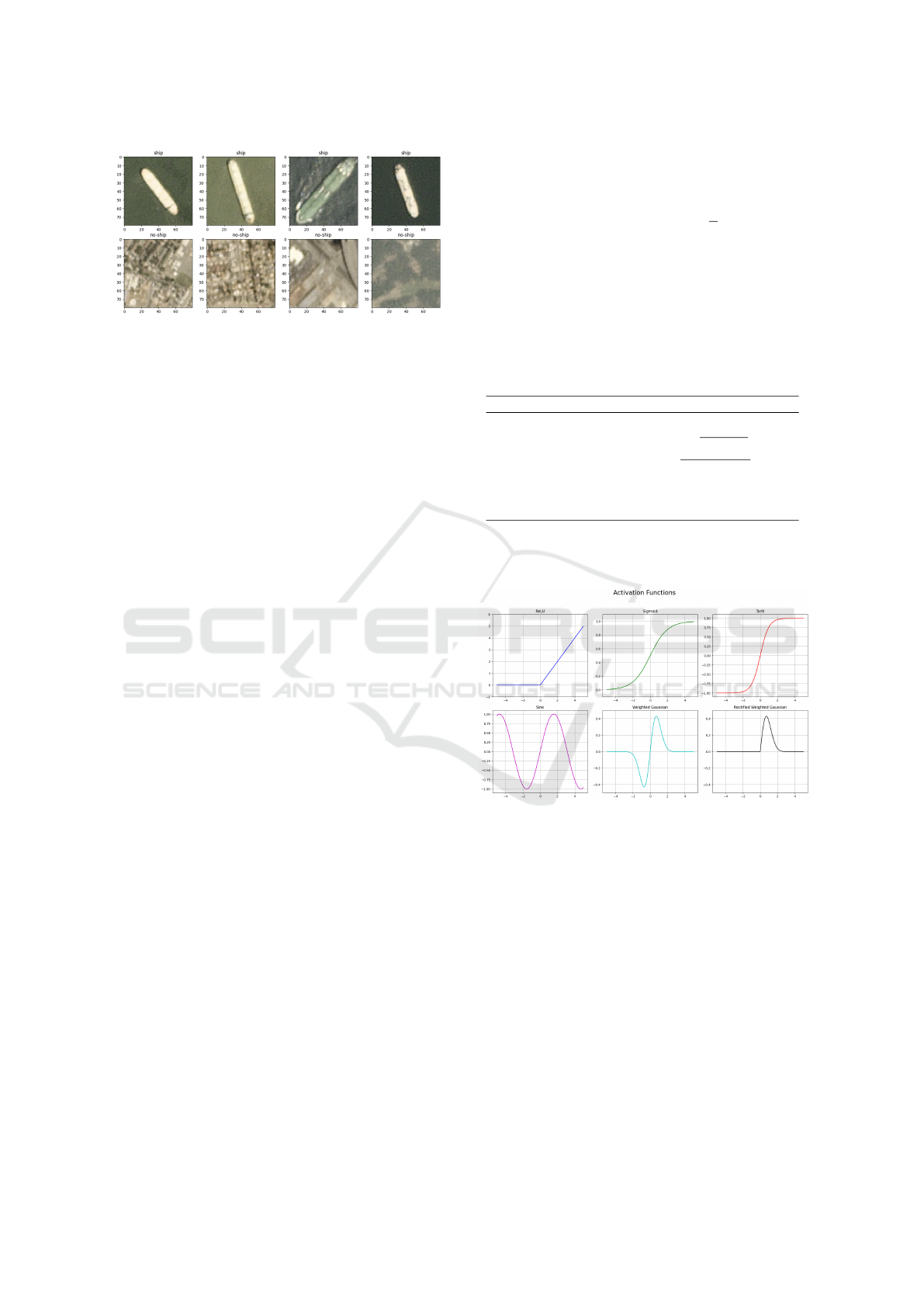
Figure 4: Example Images from the Shipsnet Dataset.

CNN architecture did not need to be a complex, state-

of-the-art model with millions of parameters. How-

ever, to be representative of large scale DNNs the

macro architecture of AlexNet was used (Krizhevsky

et al., 2012). This consists of a feature engineering

block made up of convolutional layers, then a classiﬁ-

cation block made of fully connected layers. There is

also a dropout layer with probability p between these

two blocks.

To train this CNN on the Shipsnet dataset, batched

gradient descent is used on a random 80/20 train/test

split of the 2000 samples. The loss function was

CrossEntropyLoss deﬁne in Equation (3) which mea-

sures the distance between the true labels and labels

predicted by the CNN. Adam, a version of stochas-

tic gradient descent, was chosen as the optimisation

algorithm to minimise the loss.

L (y, p) = −

∑

i=1

log(p

) (3)

A batch size of 16 samples and a learning rate

of 0.001 were chosen to balance training speed and

model generalisation. The training is completed when

either 1000 epochs are reached or the loss is less than

0.01. These values were selected as a loss of 0.01

indicates the predicted labels and true labels lie very

closely. The 1000 epochs limit serves as a safeguard

to stop algorithms that struggle to converge. From

preliminary testing, all models converge within 100

epochs so 1000 epochs was very sufﬁcient.

The hyperparameters explored in the training pro-

cess were regularisation (also known as weight-decay

in the Pytorch) and dropout probability p. Regulari-

sation adds an additional term to the loss function that

represents the squared L2 norm of the model weights

w multiplied by the regularisation coefﬁcient λ seen

in Equation (4). The aim of λ is to control the trade-

off between ﬁtting and overﬁtting by penalising large

weights (Shalev-Shwartz and Ben-David, 2014). Val-

ues of λ at 0 and 1e-4 are chosen to compare the ef-

fectiveness of regularisation. The dropout probabil-

ity p was explored in an off state, p = 0 and on state

p = 0.5. Meaning that in the on state half of the 800

features are set to 0.

L (y, p) = −

∑

i=1

log(p

) +

∥w∥

(4)

The hyperparameters explored in the CNN archi-

tecture were choice of activation function and the use

of a smart pooling. The choice of activation func-

tion determines the non-linearity of the network and

is arguably the most important hyperparameter. The

following activation functions were explored:

Table 1: Activation Functions.

Function Expression

ReLU ReLU(x) = max(0, x)

Sigmoid Sigmoid(x) =

1+exp(−x)

Tanh Tanh(x) =

exp(x)−exp(−x)

exp(x)+exp(−x)

Sinusoidal Sin(x) = sin(x)

Weighted Gaussian WG(x) = x exp(−x

)

Rectiﬁed WG RWG(x) = max(0, x exp(−x

))

Where Weighted Gaussian is deﬁned by the

acronym WG and Rectiﬁed Weighted Gaussian,

RWG.

Figure 5: Activation Functions Explored.

ReLU, Sigmoid and Tanh were chosen due to

being well established across a range of NN mod-

els. In particular ReLU is a cornerstone of many

CNNs such as AlexNet (Krizhevsky et al., 2012).

We propose the following two activation functions

speciﬁcally designed to handle SEE related errors,

the Weighted Guassian (WG) and Rectiﬁed Weighted

Guassian (RWG). The WG and RWG are bounded,

decaying and zero-at-origin as these properties are

hypothesised to aid robustness. This is because ex-

treme changes will decay to 0. The sine function is

included to assess the impact of periodicity, also be-

ing bounded.

Santos suggested the use of smartpooling, but this

has not yet been tested (Santos et al., 2019). There-

fore we test with the use of smartpooling. This CNN

A Framework for Developing Robust Machine Learning Models in Harsh Environments: A Review of CNN Design Choices

327

replaces the MaxPooling layers with smartpooling

layers that ignore unreasonable values (Rech, 2024).

Determining what is “unreasonable” can be done via

many outlier detection techniques, the simplest being

z-score or interquartile ranges. However due to the

extreme magnitudes of resulting ﬂoats from bitﬂips,

particularly at index 1 of the FP 32 architecture, an

even simpler technique was implemented. All abso-

lute values above a threshold were ignored. This aims

to produce a similar result to more advanced outlier

detection methods and serve as a proof of concept.

4.2 Error Model

With a use case and model in place, the ﬁnal step was

to create an environment to simulate and record the

effects of SEEs. The aim is to bring the simulation as

close as possible to empirical results, noting that there

is very limited research in this area.

Trained CNN Test DatasetAttack Type

Iterate though

each Weight and

Bias Tensor

Perform Attack on

Tensor

Test Perturbated

CNN Model

Record Key

Information

Reset Tensor to

Original State

Inputs

Simulation

1 2 3

Figure 6: A high level overview of the simulation environ-

ment.

The overall process for simulation follows the de-

as input and a test dataset for evaluation that is unseen

data to the CNN. Then the CNN has its weights and

biases erroneously modiﬁed (attacked) methodically.

Each attack is self-contained in a weight or bias tensor

and the tensor is reset to the original state after the at-

tack. Therefore the effect of cumulative SDCs are not

investigated, only isolated events. This was an impor-

tant decision to be made as it allows for an individual

analysis of the components that make up the CNN.

Therefore the most inﬂuential/vulnerable layers can

be identiﬁed. Future work will consider cumulative

effects. During the attack, the CNN is evaluated on

the test dataset and the following key information is

recorded: The norm deﬁned in Equation 5, name of

the layer, location of the attack, accuracy of the CNN

on the test dataset, number of parameters attacked

and proportion of parameters attacked in the tensor.

norm(t

) = |t

−t

| (5)

To allow a fair comparison between different CNN

model parametisations the bitﬂip index and spatial

distribution must be consistent. Single, line and

rectangle are common spatial distributions of SDCs.

However, after preliminary exploration into simula-

tions with these distributions, the line distribution was

found to be catastrophic to the performance of the

CNN. This allows for no comparison between param-

etisations so is unfortunately not a feasible simulation

for a smaller CNN. This critical reduction in perfor-

mance can be attributed to the low number of param-

eters in the CNN where feature channels are as small

as 8. It will likely be more applicable to larger CNNs.

The rectangle distribution is an even more destructive

extension of the line distribution so was also not con-

sidered. This does not pose a problem as SEU is the

most common result of SEEs.

To provide a comprehensive analysis of SEUs, the

process in Figure 6 was repeated. The SEU simula-

tion iterates through all 7634 parameters of the CNN,

providing the most thorough analysis possible. This

rigarous approach was not possible for any MBU sim-

ulation as the number of combinations (subsets) that

can be made from 7634 parameters is 2

7634

, which is

approximately 10

2290

and exceeds practical computa-

tional capabilities.

Representation of a MBU was still desired so we

proposed an approach that used a Gaussian process to

propagate a SEU into an MBU. Spatial distributions

of errors inspired by propagation are not new and have

been implemented by others (Bolchini et al., 2023) to

simulate SEEs.

Algorithm 1 outlines the generation of indices to

be attacked during the MBU simulation. The num-

ber of indices attacked is controlled by the standard

deviation and was varied during the simulation. Due

to the random nature of Algorithm 1, it is repeated

within each layer of the CNN. The number of repe-

titions is the minimum of; the number of parameters

in the layer or one hundred. This mitigates against

repetition of the same indices being selected in small

tensors such as the biases which may contain less than

10 parameters.

Require: Tensor x, Index i, Standard Deviation σ

1: Flatten x into a vector of n values

2: Generate an array A of normal distribution values

with mean i, standard deviation σ, and length n

3: Normalize the values in A between 0 and 1

4: Generate an array B of random uniform values

between 0 and 1 with length n

5: return boolean array C where

= (B

< A

) ∀ j ∈ [0, n)

Algorithm 1: MBU Index Selection Algorithm.

Figure 3 shows that the index of the bitﬂip can

cause a near-zero change or change to the extremities

ICAART 2025 - 17th International Conference on Agents and Artiﬁcial Intelligence

328

of the FP32 architecture. Testing every single index

would be an inefﬁcient use of resources as, aside from

index 0, the MAE is monotonically decreasing as the

bit index increases. This allows for the assumption

that results relating to the bitﬂip index can be inter-

polated without exhaustive testing. Therefore 7 of the

32 indices were selected to be investigated. The sign

bit, three exponent bits (1,3,6) and three mantissa bits

(10,15,21) were the indices selected. This gives a fair

representation of the three parts of the FP32 architec-

ture. The mantissa bits are skewed towards the lower

indices due to the decreasing change in MAE. This is

because it is expected that the impact would be mini-

mal as the MAE approaches 0.

To summarise the simulation environment, both

SEU and MBU methodologies were outlined. The

SEU simulation exhaustively tests all parameters and

the MBU attacks a selection of parameters propagat-

ing from a single SEU. Regarding the bitﬂipping, 7 of

the total 32 bits in the FP32 architecture were tested.

All this results in the following number of simula-

tions:

SEU Simulations:

• Factors: 7,634 parameters, 6 activation functions,

7 bit indices, 2 pooling layers, 2 dropout, 2 regu-

larization

• Total: 7, 634 × 6 × 7 × 2 × 2 × 2 = 2, 565, 024

MBU Simulations:

• Factors: 458 initializations, 5 standard deviations,

6 activation functions, 7 bit indices, 2 pooling lay-

ers, 2 dropout, 2 regularization

• Total: 458 × 5 × 6 × 7 × 2 × 2 × 2 = 769, 440

5 EVALUATION

A total of 3,334,464 attacks were simulated follow-

ing the methodology in Chapter 4. 2,565,024 were

performed using the SEU simulation and the remain-

ing 769,440 for the MBU simulation. Table 2 outlines

the distribution of the number of simulations and the

number of single bitﬂips i.e. SEU attacks is greater

than the number of SEU simulations. This is because

a number of the MBU simulations, with a particularly

low standard deviation, result in only one index being

attacked.

To evaluate how the different model parameter

settings affect the model’s performance with different

error models, we use the test delta, computed as the

difference between the test accuracy before and after

the errors are introduced.

5.1 Simulation

Table 3 offers a summary of the key simulation and

CNN parameters against the test delta. It shows that

there exists complex interactions between these pa-

rameters, where one parameter may only be bene-

ﬁcial in the presence of one or more other parame-

ters. Therefore, the analysis is visualised with many

multidimensional ﬁgures. The discussion starts with

the simulation parameters, then delves into the CNN’s

learning parameters and architectural design.

Bitﬂip location was the most important factor to

the test delta. Figure 8 shows the non-zero test delta

rate at each index. In the mantissa, only 1% of the

simulations had a non-zero test delta, also known as

critical error, with a maximum of only 0.0475 test

delta. Also, the 21st index had zero test delta across

all 476,352 simulations. It is fair to say that all sub-

sequent indices 22-32 will also have zero test delta.

Therefore, assuming a uniform distribution across the

indices ﬂipped, it can be said that a third of bitﬂips

have a zero test delta, or in other words, no impact.

In the exponent, 27% of the simulations had a non-

zero test delta with the 1st index having the most im-

pact at 52%. It is surprising however, that the 3rd

index had less impact than the 6th. This is due to the

3rd index having a lower average norm than the 6th.

The sign bit had a 12% non-zero test delta placing it

ﬁrmly between the exponent and mantissa. Figure 7

supports this as the test delta in the conv1.bias layer

is 300 times smaller in the mantissa than the sign and

exponent. These results fall in line with the hypothe-

sis that the magnitude of the difference caused by the

bitﬂip is proportional to the impact on the wider CNN.

The Layer attacked within the CNN was another

signiﬁcant factor to the test delta. Figure 8 shows a

U-shaped pattern for average test delta with respect

to the forward propagation order of the CNN layers.

This points towards the ﬁrst and ﬁnal layers of the

CNN architecture being most sensitive to perturba-

tions. The bias layers also exhibit higher test deltas

than the weight layers suggesting they are more sen-

sitive, a result that was also found by Bolchini et al.

(Bolchini et al., 2022). This may be explained by the

formulation in Equation (2) where the bias is a direct

addition to the output vector whereas the weights con-

tribute via a sum-product with the input. However,

Figure 7 points towards a contradiction to this belief.

It shows that the proportion attacked in each layer

varies a signiﬁcant amount with bias layers reaching

up to 100% and the weight layers reaching no more

than 30%. Therefore the gradient in Figure 7 could

be a more accurate measure of the sensitivity of each

layer as it represents how the model degrades with

A Framework for Developing Robust Machine Learning Models in Harsh Environments: A Review of CNN Design Choices

329

Table 2: Summary of Simulations Performed Following the Methodology in Chapter 4.

Bitﬂips per Simulation SEU (1) 2-4 5-9 10-14 15-24 25-39 40+

Total # Simulations 2,583,531 192,073 121,599 123,349 96,573 90,157 127,182

Table 3: Average test delta of different CNNs with various setups. The minimal value in each row is marked with an asterisk

(*) and global minima with (**).

Dropout Weight Decay Model Standard Activation Functions Proposed Act. Func.

ReLU Sigmoid Tanh Sine WG RWG

0.0 0.0 CNN 0.02760 0.01784 0.01758 0.01773 0.01347 0.01234*

SmartPoolCNN 0.01809 0.01774 0.01756 0.01750 0.01363 0.01227*

0.0001 CNN 0.02755 0.01731 0.01669 0.02002 0.01318 0.01275*

SmartPoolCNN 0.02126 0.01738 0.01667 0.02023 0.01333 0.01260*

0.5 0.0 CNN 0.02418 0.01834 0.01573 0.01853 0.01322 0.01020**

SmartPoolCNN 0.02241 0.01828 0.01567 0.01857 0.01335 0.01021*

0.0001 CNN 0.02155 0.01892 0.01702 0.01700 0.01314 0.01126*

SmartPoolCNN 0.01931 0.01900 0.01718 0.01689 0.01313 0.01129*

respect to the proportion of the layer attacked. Exam-

ining the gradient ﬁnds that the weight matrix in the

ﬁrst convolutional layer would be the most sensitive

layer with respect to proportion. The most important

takeaway from Figure 7 is that there is a clear linear

relationship between the proportion of the layer at-

tacked and test delta, conﬁrming what Santos stated

(Santos et al., 2019). This is also reﬂected in Figure

8 where the SEU simulations have a lower test delta

than the MBU simulations.

Dropout was a factor during the training of the

models with the purpose of improving robustness.

Averaged over all the results it reduced the average

test delta from 0.0172 to 0.0164. Figure 9 summarises

the impact per activation function and there was a

reduction in test delta across all activation functions

bar the sigmoid function. During training, the sig-

moid function also faced difﬁculties with the use of

dropout. It is not clear why this is the case and would

be an area of future work. The two rectiﬁed functions

had the largest decrease in test delta. This could be

due to the sparsity of rectiﬁed functions and dropout

further amplifying the sparsity, forcing a multitude of

neural pathways to form, similar to ensemble models

which are naturally robust.

Regularisation was the least impactful parame-

ter to the test delta having an insigniﬁcant average in-

crease to the test delta of 0.0001 over all the results.

Regularisation only had a beneﬁt when the ReLU ac-

tivation function and dropout were used, shown in Ta-

ble 3. The reason for this could follow a similar trail

of thought to the interaction between the ReLU acti-

vation function and dropout, further reinforcing more

neural pathways.

The choice of Activation Function has been

lightly touched upon in the last two paragraphs and

was the most signiﬁcant factor to test delta within the

CNN architecture. Moving left to right in Table 3,

the activation function with the highest test delta was

ReLU. This was unsurprising as all other activation

functions were bounded, so extreme values passed

though bounded functions do not propagate through

the CNN. The bounding of values also explains why

the use of smart pooling was only effective with the

ReLU function, showing a 16% reduction to the av-

erage test delta. The well known bounded activa-

tion functions, sigmoid, tanh and sine achieved simi-

lar levels of average test delta, around 0.017 and tanh

reached an even lower 0.015 test delta with dropout

and no regularisation. The proposed activation func-

tions consistently achieved a lower test delta across all

training parameters. An explanation for this could be

the decaying property of the WG function. This cre-

ates an “active” region so that only a small range of

values produce a non-zero output, essentially bound-

ing the range of values in a similar manner to smart-

pooling. The RWG performs even better than the WG

function and has an even smaller “active” region. The

best model, at 0.01 average test delta, used the RWG

activation function, dropout at p = 0.5, no regularisa-

tion and no smartpooling. However the difference be-

tween using smartpooling or not was negligible. This

was a 58% reduction in error over the use of ReLU.

The Norm was a measure of the difference be-

tween the original tensor and attacked tensor, deﬁned

in equation (5). It is a direct reﬂection of the bit index

and number of bitﬂips. Figure 10 shows the relation-

ship between the log of the norm and the test delta

across the eight layers in the CNN. As expected, there

is a positive correlation between the log norm and the

test delta across all layers. In some of these layers

a slight S-shape can be observed. This can point to-

wards the idea that the relationship is not strictly lin-

ear. Therefore, there may be resilience to small per-

turbations up to a critical norm value, then a satura-

tion point where the layer stops functioning so fur-

ICAART 2025 - 17th International Conference on Agents and Artiﬁcial Intelligence

330

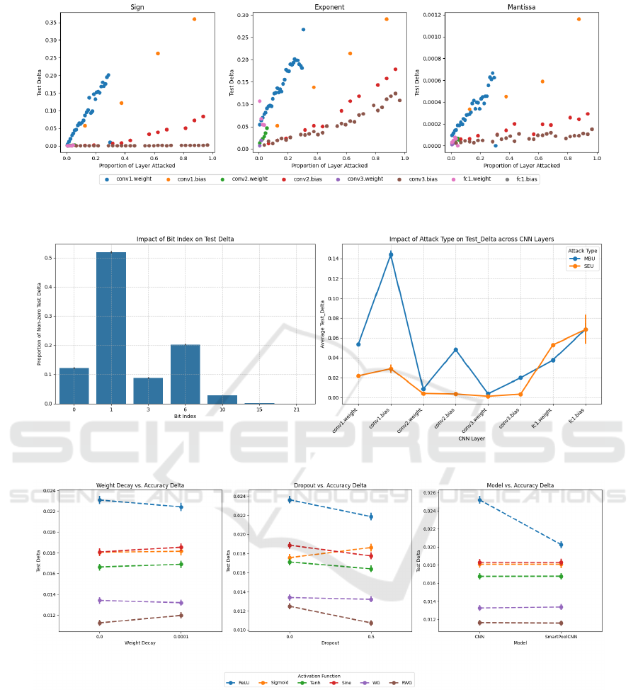
Figure 7: The average test delta in the Sign (left), Exponent (middle), Mantissa (right) part of the FP32 architecture against

the portion of the layer attacked.

Figure 8: Proportion of non-zero Test Deltas across Bit Indices (left), Average Test Delta across layers in the CNN (right).

Figure 9: The average test delta of Regularisation (left), Dropout (middle), Model (right) across the six activation functions.

ther attacks have nothing to degrade. The horizontal

grey lines represent test delta values of 0.01 and 0.1

and can be used to assess the sensitivity of each layer.

The ﬁrst weight matrix breaks these thresholds with

the smallest log norms which reinforces the idea that

is the most sensitive layer.

5.2 Testing AlexNet

A ﬁnal test was performed using AlexNet. It explored

the novel RWG activation function and smartpool-

ing. Due to computational constraints the CIFAR-

100 dataset was used and includes 60,000 images with

100 different labels (Krizhevsky, 2009). Therefore the

ﬁnal layer of AlexNet had to be resized to the 100

classes instead of 1000. Also the images in CIFAR-

100 were scaled up to 224x224 pixels and normalised.

A Framework for Developing Robust Machine Learning Models in Harsh Environments: A Review of CNN Design Choices

331

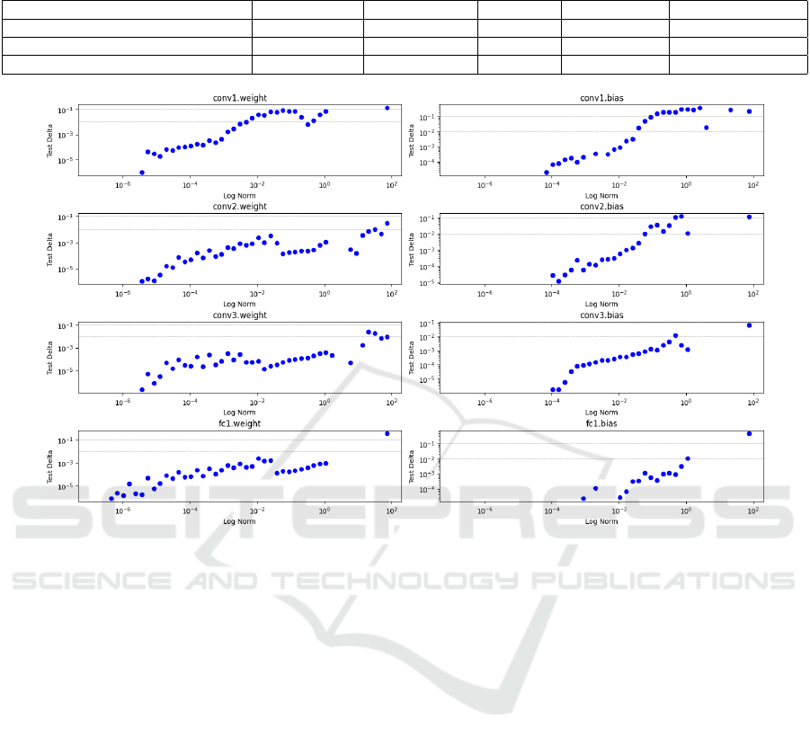
Table 4: Comparison of Alexnet models on CIFAR-100. *Training epochs from weights copied from training Alexnet with

ReLU.

Model Type Test Accuracy SEU Accuracy Test Delta # Simulations # Training Epochs

Alexnet with ReLU 0.717100 0.312881 0.404219 160 20

Alexnet with RWG

0.01

0.742900 0.663311 0.079589 160 20* + 5

Alexnet with ReLU and smartpooling 0.707600 0.403594 0.304006 160 20*

Figure 10: Log of the Norm against test delta in each layer of the CNN.

It was quickly realised that training AlexNet was

computationally expensive so transfer learning was

used. A pretrained version of AlexNet was down-

loaded and, after transfer learning, achieved a 71.7%

test accuracy shown in Table 4. A special variant of

the RWG function deﬁned in Equation (6) allowed

the use of transfer learning from AlexNet (which uses

ReLU) to a version of AlexNet with the RWG

ac-

tivation function. This further transfer learning was

successful and additional training epochs added a few

extra percent to the test accuracy. Smartpooling had

the advantage of not needing any further training, just

the replacement of the pooling layers with smartpool-

ing layers. This did however reduce the test accuracy

by 1%.

RWG

(x) = max(0, x exp(−Kx

))

=⇒ lim

K→0

RWG

(x) = ReLU(x)

(6)

With only 160 SEUs, equating to 10 SEUs per

layer in AlexNet, this is far from a thorough exper-

iment. Additionally, only the ﬁrst exponent bit was

ﬂipped as it has the highest impact. Therefore the

weight these results carry is up to the reader’s judge-

ment. However, there is an indicative difference be-

tween Alexnet with ReLU, Alexnet with RWG

0.01

and Alexnet with ReLU and smartpooling.

6 CONCLUSION

To conclude, a framework to simulate and test the ef-

fects of SEEs was built with the Pytorch library. A

third of simulated SEEs have minimal impact due to

small changes in the mantissa. There exists a linear

relationship between the proportion of the layer at-

tacked and test delta. The use of dropout during train-

ing improves robustness but regularisation does not.

Smartpooling layers were beneﬁcial in conjunction

with ReLU. The proposed activation function RWG

was the most robust to simulated SEEs and transfer

learning can be used to convert CNNs using ReLU to

RWG

. Small norms (e.g. less than 10

−6

) have mini-

mal impact on the test delta. Future work will include

validated error models and evaluating robustness with

state-of-the-art models.

ICAART 2025 - 17th International Conference on Agents and Artiﬁcial Intelligence

332

REFERENCES

Badaroglu, M. (2021). More moore. In 2021 IEEE Inter-

national Roadmap for Devices and Systems Outbriefs,

pages 01–38.

Binder, D., Smith, E. C., and Holman, A. B. (1975). Satel-

lite anomalies from galactic cosmic rays. IEEE Trans-

actions on Nuclear Science, 22(6):2675–2680.

Bolchini, C., Cassano, L., Miele, A., and Nazzari, A.

(2022). Selective hardening of cnns based on layer

vulnerability estimation. In 2022 IEEE International

Symposium on Defect and Fault Tolerance in VLSI

and Nanotechnology Systems (DFT), pages 1–6.

Bolchini, C., Cassano, L., Miele, A., and Toschi, A. (2023).

Fast and accurate error simulation for cnns against soft

errors. IEEE Transactions on Computers, 72(4):984–

997.

Bosio, A., Bernardi, P., Ruospo, A., and Sanchez, E. (2019).

A reliability analysis of a deep neural network. In

2019 IEEE Latin American Test Symposium (LATS),

pages 1–6.

Bureau, A. T. S. (2008). In-ﬂight upset 154 km west of

learmonth. Australian Transport Safety Bureau.

Hammell, R. (2018). Ships in satellite imagery.

Hari, S. K. S., Tsai, T., Stephenson, M., Keckler, S. W., and

Emer, J. (2017). Sassiﬁ: An architecture-level fault

injection tool for gpu application resilience evalua-

tion. In 2017 IEEE International Symposium on Per-

formance Analysis of Systems and Software (ISPASS),

pages 249–258.

Hornik, K., Stinchcombe, M., and White, H. (1989). Multi-

layer feedforward networks are universal approxima-

tors. Neural Networks, 2(5):359–366.

Huang, K.-H. and Abraham, J. A. (1984). Algorithm-based

fault tolerance for matrix operations. IEEE Transac-

tions on Computers, C-33(6):518–528.

IBM (2024). Neural networks. https://www.ibm.com/

topics/neural-networks. Accessed: 2024-08-26.

Ibrahim, Y., Wang, H., Liu, J., Wei, J., Chen, L., Rech, P.,

Adam, K., and Guo, G. (2020). Soft errors in dnn ac-

celerators: A comprehensive review. Microelectronics

Reliability, 115:113969.

IEEE754 (2019). IEEE Standard for Floating-Point Arith-

metic. IEEE Std 754-2019 (Revision of IEEE 754-

2008), pages 1–84.

Krizhevsky, A. (2009). Learning multiple layers of features

from tiny images. Technical Report.

Krizhevsky, A., Sutskever, I., and Hinton, G. E. (2012).

Imagenet classiﬁcation with deep convolutional neu-

ral networks. In Pereira, F., Burges, C., Bottou, L.,

and Weinberger, K., editors, Advances in Neural In-

formation Processing Systems, volume 25. Curran As-

sociates, Inc.

Lu, Z., Pu, H., Wang, F., Hu, Z., and Wang, L. (2017). The

expressive power of neural networks: A view from the

width.

Moore, G. (1998). Cramming more components onto inte-

grated circuits. Proceedings of the IEEE , 86(1):82–85.

Peterson, E. (2011). Introduction, chapter 1, pages 1–12.

John Wiley & Sons, Ltd.

Pilla, L. L., Rech, P., Silvestri, F., Frost, C., Navaux, P.

O. A., Reorda, M. S., and Carro, L. (2014). Software-

based hardening strategies for neutron sensitive fft al-

gorithms on gpus. IEEE Transactions on Nuclear Sci-

ence, 61(4):1874–1880.

Radford, A., Wu, J., Child, R., Luan, D., Amodei, D., and

Sutskever, I. (2019). Language models are unsuper-

vised multitask learners.

Rech, P. (2024). Artiﬁcial neural networks for space and

safety-critical applications: Reliability issues and po-

tential solutions. IEEE Transactions on Nuclear Sci-

ence, 71(4):377–404.

Rech Junior, R. L., Malde, S., Cazzaniga, C., Kastriotou,

M., Letiche, M., Frost, C., and Rech, P. (2022). High

energy and thermal neutron sensitivity of google ten-

sor processing units. IEEE Transactions on Nuclear

Science, 69(3):567–575.

Santos, F. F. d., Pimenta, P. F., Lunardi, C., Draghetti, L.,

Carro, L., Kaeli, D., and Rech, P. (2019). Analyzing

and increasing the reliability of convolutional neural

networks on gpus. IEEE Transactions on Reliability,

68(2):663–677.

Science and Technology Facilities Council (2024). Chipir.

[Accessed 01-10-2024].

Sequin, C. and Clay, R. (1990). Fault tolerance in artiﬁ-

cial neural networks. In 1990 IJCNN International

Joint Conference on Neural Networks, pages 703–708

vol.1.

Shalev-Shwartz, S. and Ben-David, S. (2014). Understand-

ing Machine Learning: From Theory to Algorithms.

Cambridge University Press. Chapter 13: Regulariza-

tion and Stability.

Su, F., Liu, C., and Stratigopoulos, H.-G. (2023). Testabil-

ity and dependability of ai hardware: Survey, trends,

challenges, and perspectives. IEEE Design & Test,

40(2):8–58.

VAN ALLEN, J. A., LUDWIG, G. H., RAY, E. C., and

McILWAIN, C. E. (1958). Observation of high in-

tensity radiation by satellites 1958 alpha and gamma.

Journal of Jet Propulsion, 28(9):588–592.

Wallmark, J. T. and Marcus, S. M. (1962). Minimum

size and maximum packing density of nonredundant

semiconductor devices. Proceedings of the IRE,

50(3):286–298.

A Framework for Developing Robust Machine Learning Models in Harsh Environments: A Review of CNN Design Choices

333