Noisemaker 3D: Comprehensive Framework for Mesh Noise Generation

Vladimir Mashurov

1,2,∗ a

, Vasilii Latonov

1,∗ b

, Anastasia Martynova

1,3 c

and Natalia Semenova

1,4 d

Sberbank PJSC, 19 Vavilova St., Moscow 117312, Russia

ITMO University, Kronverkskiy Lane 49, Saint-Petersburg, 197101, Russia

HSE University, 20 Myasnitskaya St., Moscow 101000, Russia

AIRI, Kutuzovsky prospect 32 bld 1, Moscow 121170, Russia

Keywords:

Mesh Denoising, 3D Noise Generation, Synthetic Dataset, Topological and Node Noise.

Abstract:

In this article, we present a comprehensive library for generating node and topological noise in meshes. The

library provides a versatile tool for creating corrupted mesh datasets, which are essential for learning-based

denoising algorithms. Our main contributions include cluster and patch noise generation techniques for mesh

topology corruption. Cluster generation supports two modes: separated and merged clusters. We also compare

the node noise generated by the library to real noise from a scanned object dataset. Finally, we create a noisy

object dataset using the library and test it with ﬁlter-based and machine learning-based denoising methods.

1 INTRODUCTION

The 3D scene reconstruction problem is a common

challenge in various ﬁelds (Ma Z., 2018). Solving this

problem often requires specialized technical support

and complex software for data processing. Advanced

3D reconstruction algorithms use input data from

various sensors, such as cameras, RGB-D cameras,

and infrared cameras, to generate a reconstructed 3D

model of the scene. The 3D ﬁgure is represented in

various ways, including polygon meshes and voxel

grids. However, despite the use of advanced scan-

ning technologies and state-of-the-art signal process-

ing algorithms, the reconstructed scene is still prone

to errors. As a result, the virtual scene may differ

from the original (Kamberova G., 1997) real-world

one, making it unsuitable for immediate use in subse-

quent graphics pipelines.

In this article, we discuss various types of errors

that can occur in triangle meshes generated by 3D

scene reconstruction algorithms. These errors are re-

ferred to as noise. The process of eliminating noise

from a triangle mesh is known as denoising. The aim

https://orcid.org/0009-0000-1148-8425

https://orcid.org/0000-0002-7810-8033

https://orcid.org/0009-0007-7003-5822

https://orcid.org/0000-0003-4189-5739

∗

These authors contributed equally

of removing noise from a 3D scene is to create a re-

constructed 3D model that is as similar to the original

real-life scene as possible.

Modern research has developed a wide range of

denoising algorithms for triangle meshes. These al-

gorithms can be divided into two main categories.

The ﬁrst category includes classical methods, which

are represented by ﬁlters and do not require train-

ing (Wang P.-S., 2016).

The second group includes learning-based meth-

ods for mesh denoising (Botsch J., 2022), (Zhao W.,

2021) and shape reconstruction (Litany O.,

2018), (Dai A., 2017). These methods require

sufﬁcient number of clear (ground-truth) meshes and

their noised versions. The greater the variety of noise

in the training dataset, the better trained algorithm

can deal with noise.

In this paper, we present a library of noise gener-

ation algorithms that can generate node and topolog-

ical noise for any triangle mesh. We have also pro-

vided our library with probing based on ﬁve denois-

ing approaches, and have applied learning- and non-

learning-based methods to the noised datasets gener-

ated by our library.

Our motivation is to provide a comprehensive

toolkit for a variety of noise generation methods

on 3D meshes, to help researchers avoid the time-

consuming process of searching for and conﬁguring

separate approaches. Additionally, we aim to address

Mashurov, V., Latonov, V., Martynova, A. and Semenova, N.

Noisemaker 3D: Comprehensive Framewor k for Mesh Noise Generation.

DOI: 10.5220/0013155800003912

Paper published under CC license (CC BY-NC-ND 4.0)

In Proceedings of the 20th Inter national Joint Conference on Computer Vision, Imaging and Computer Graphics Theory and Applications (VISIGRAPP 2025) - Volume 2: VISAPP, pages

667-674

ISBN: 978-989-758-728-3; ISSN: 2184-4321

667

the issue of the non-reproducibility of open-source

implementations.

Our main contribution can be summarized as fol-

lows:

• We introduce a new library of algorithms for gen-

erating mesh noise. This library provides an efﬁ-

cient way to create a large-scale dataset, with high

computational speed. Additionally, we have gen-

erated a dataset using our algorithmic approach..

• We provide a probing of our dataset and a com-

parison with other relevant dataset.

2 MESH NOISE OVERVIEW

We consider two types of noise that researchers usu-

ally face in triangle meshes. The ﬁrst type is called

node noise (I., 2013). The most common cause of

this type of noise is low precision of the sensors used

for 3D scene capture.

The second type is topological noise or holes.

This causes the absence of small or signiﬁcant frag-

ments of the mesh. The most common cause of these

holes is occlusion. Another reason is the inability to

capture the ﬁgure from all necessary angles. More-

over, holes can appear in the reconstructed model due

to low reﬂectivity (Davis J., 2002). Removing this

type of noise is called hole ﬁlling (Zhong M., 2016)

or shape completion.

3 NOISE GENERATION

FRAMEWORK

In this section, the noise generation algorithms imple-

mented in our library are presented. These algorithms

are divided into node noise and topological noise gen-

eration.

3.1 Node Noise

3.1.1 Random Noise

Node random noise is modeled with probability distri-

butions (Nguyen C. V., 2012). By varying the distri-

bution parameters, any required noisy surface can be

achieved. The probability distribution function (PDF)

deﬁnes the distance of each node’s shift.

We provide the following PDF for node noise

generation: Gaussian, Laplace, Exponential, Ex-

treme value, Gamma, Log normal, Uniform, Weibull,

Cauchy, Fisher, Student and Chi squared distribu-

tions.

The second part of the node noise is the direction

of the shift. This can be deﬁned randomly or as the

normal of a vertex.

3.1.2 Impulsive Noise

The Impulsive noise

supposes that a speciﬁed range

of vertices is shifted. The Gaussian distribution is

used to calculate vertices offsets. The number of ver-

tices to generate noise can be speciﬁed (the number

must be less or equal than range size).

Some examples of node noise generated with the

algorithms developed are depicted on Figure 1.

3.2 Topological Noise

We provide the following topological noise genera-

tion algorithms:

• Random vertex removing algorithm

• Cluster algorithm with random removing center

• Cluster algorithm with speciﬁed removing center

• Set of clusters removing algorithm

• Patch noise

Let us denote the graph that represents the mesh

we are considering with G = (V,E,F), where V is the

set of vertices, E the set of edges, which are pairs

of vertices, and F the set of faces, each of which is

bounded by three edges. Each face is in the shape of

a triangle.

3.2.1 Random Noise

The Random algorithm is quite simple: it removes

each mesh vertex with a speciﬁed probability.

3.2.2 Cluster Noise

The Cluster noise algorithm allows to remove a set

of vertices in the vicinity of a speciﬁed vertex which

is called removing center. Let us give the descrip-

tion of a cluster. The vertex c is the center vertex that

is removed. Let us denote by d(v,c) the number of

edges in the shortest path between vertex v ∈ V and

the cluster center c. We deﬁne by R the cluster radius.

If d(v,c) ≥ R than vertex v is not removed. The ver-

tices with d(v,c) < R are deleted with a probability

P(v) that is calculated with the following method.

Consider the Gaussian distribution with mean µ =

0 and standard deviation σ. We denote the corre-

sponding probability density function by 1:

We used a part of implementation of Impulsive noise

from GCN-Denoiser

VISAPP 2025 - 20th International Conference on Computer Vision Theory and Applications

668

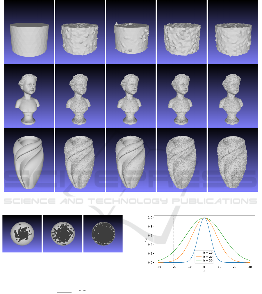
(a) GT (b) Exponential (c) Gamma (d) Gaussian (e) Weibull

Figure 1: Results of node noise generation applied to cylinder, bust and vase100K.

(a) (b) (c)

Figure 2: Topological noise clusters generated on the sphere

with σ = 0.5 and different h parameters: h = 10 (b), h = 20

(c), and h = 30 (d).

f (x, σ) =

√

2π

−

(

)

. (1)

Zero mean is required to make the highest proba-

bility of removing of vertices that are the closest to c.

We calculate d

= d(v, c) for a vertex v. The probabil-

ity to remove vertex v equals f (d

/h,σ), where h is a

special divider that determines how close to the peak

of the normal distribution the probabilities should be

chosen. The examples of cluster noise depending on

h is displayed on the Figures 2 and 3.

Figure 3: The Gaussian distributions with different h di-

viders, µ = 0 and σ = 0.5. The dashed vertical lines deﬁne

the interval [−20,20] that is used for clusters generation on

Figure 2. The bigger h the higher probability of faces re-

moving near the border of cluster.

Thus, the topological noise cluster C is deﬁned as

C = C(c,σ,h,R). The d(v, c) calculation is performed

via Breadth First Search (BFS) algorithm with the

start point at c vertex which can be speciﬁed by vertex

index or selected randomly.

Noisemaker 3D: Comprehensive Framework for Mesh Noise Generation

669

(a) (b)

(c)

(d)

Figure 4: Consider R = 2 and D = 4. The clusters are gen-

erated in the following way: a) The ﬁrst cluster is generated

randomly. b) The second cluster is generated so the distance

between centers equals D. c) The distance between third

cluster centers and the others centers is maximal if strat-

egy S(c

k+1

) → max is used. d) The distance between fourth

cluster centers and the others centers is minimal if strategy

S(c

k+1

) → min is used.

3.2.3 Set of Clusters Noise

The Set of Clusters algorithm generates the speciﬁed

number K of noise clusters C, where each cluster is

deﬁned as described above. The clusters are gener-

ated sequentially one by one. Each cluster is deﬁned

as C

= C(c

,σ,h,R); i = 1,.. . ,K. This algorithm re-

quires two additional parameters in comparison with

the previous one. The ﬁrst parameter which is labeled

by D is a desired distance between centers of each

pair of clusters. The second one is a variable that de-

scribes a strategy of clusters centers selection. We de-

ﬁne a function of sum distance between a new i + 1-th

center point and all previous ones with 2:

S(c

k+1

) =

∑

i=0

d(c

c+1

). (2)

There are two strategies of c

k+1

selection:

S(c

k+1

) → max and S(c

k+1

) → min.

The following algorithm was implemented. Let us

denote as isMax a boolean variable that deﬁnes if max

S(c

k+1

) is required. The idea of the algorithm consists

of BFS modiﬁcation. We start BFS K times. In the

end of i-th BFS the c

i+1

vertex is obtained. The ﬁrst

BFS is started from randomly selected vertex which

is set as c

. We introduce a priority queue structure

which is labeled as prQueue. This queue contains

pairs (v, S(v)). The comparison operator is adjusted

to make highest priority either pair with the smallest

S(v) if minimization is required or the pair with the

biggest S(v) if maximization is required. The c

i+1

selected randomly from the candidates with the best

S(v).

Input: C = (V,E,F),c

Parameter: K, R, D,σ,h

Output: verticesToDelete Let k = 0,c

= c

;

Let verticesToDelete =

while k < K do

prQueue.clear();

totalDistMap.clear();

queue.push(c

);

while !queue.empty() do

vCurr = queue. f ront();

Calculate d(c

,v) for vertices v

adjacent to vCurr;

if d(c

,v) > K ·R then

continue;

end

Let totalDistMap[v]+ = d(c

,v);

if d(c

,v) == D then

prQueue.push(v,totalDistMap[v]);

end

queue.push(v);

if d(c

,v) < R then

Calculate p = f (d

/h,σ);

isDelete =

GenerateBernoulli(p);

if d(c

,v) < R then

verticesToDelete.insert(v);

end

k + +;

= prQueue.top();

end

return verticesToDelete;

Algorithm 1: Set of clusters generation.

The strategies for selecting c

k+1

provide a speciﬁc

sequence for generating clusters. These strategies are

illustrated in Figure 4. The output of the algorithm is

a list of vertices that need to be removed. Figure 5

shows an example of the result.

VISAPP 2025 - 20th International Conference on Computer Vision Theory and Applications

670

3.2.4 Patch Noise

The Patch noise algorithm enables faces removing de-

pending on theirs position in relation to neighboring

faces. The small convex and concave fragments are

often missed. We introduce the speciﬁc noise model

to search such difﬁcult faces. we use the normal vot-

ing tensor (Yadav S.K., 2018) approach.

A patch p

that refers to the face f

∈F is a face f

and a set of faces in

R-ring neighborhood. The

R is a

radius that determines a size of patch.

Consider an arbitrary face and its patch. We de-

note the face’s normal as ¯n and the radius-vector of

the face center’s as ¯c. Let us introduce a vector

¯c

′

= ¯c

− ¯c, where ¯c

is a radius-vector of j-th face

in neighborhood of considered face. Here we label all

neighboring faces with j = 1,.. . ,N.

For each j-th face in neighborhood we denote by

the area of the face. We introduce the following

notions:

max

= max

j=1,...,N

, µ

max

exp(−||¯c

′

||/σ), (3)

where σ deﬁnes an importance of faces depending on

theirs distance from central face. Besides it we intro-

duce n

′

= 2( ¯n

· ¯w

) ¯w

− ¯n

, where ¯w

= [ ¯c

′

× ¯n

]× ¯c

′

The normal voting tensor is deﬁned by the formula 4:

T =

∑

j=1

′

. (4)

The eigenvalues of this tensor (λ

,λ

) are nor-

malized and sorted in the decreasing order: λ

≥λ

≥

. The face can be classiﬁed according to its patch

eigenvalues. The special restricting constants are used

to classify faces: ˆc

,k = 1,. ..,5. The faces are clas-

siﬁed as follows (Shen Y., 2022):

• If λ

< ˆc

and λ

< ˆc

then face classiﬁed as Plane

• If λ

> ˆc

and λ

< ˆc

then face classiﬁed as Edge

• If λ

> ˆc

then face classiﬁed as Corner

• In all other cases face is classiﬁed as Transitional

The Patch noise algorithm selects randomly the

speciﬁed portion of all faces from speciﬁed classes

and deletes them with neighboring faces. The number

of rings of neighboring faces to delete is also speci-

ﬁed.

Some examples of topological noise generated

with the algorithms developed are shown on Figure

More examples of node and topological noise are

provided in supplementary materials in our GitHub

repository.

The time consuming report is provided in supple-

mentary materials in our GitHub repository. A per-

sonal computer with Intel(R) Core(TM) i5-4670 CPU

3.40 GHz was used for library testing.

4 GENERATED DATASET

OVERVIEW

We used a dataset from (Wang P.-S., 2016) for our

tests

. This dataset was chosen because it is open-

source and contains both small and large meshes with

various geometric features. The Synthetic subset was

used to create examples of noisy meshes. We selected

three groups of meshes for testing:

• Complicated geometry models: armadillo, Chi-

nese lion and gargoyle;

• CAD models: block, joint and turbine Lp;

• Models with smooth surface: bumpy torus, fertil-

ity and kitten;

These models are selected to diversify the geome-

try as much as possible.

We choose three types of noise for testing. Each

type is used with three different parameters, resulting

in 9 noisy models from each ground truth. The types

of noise used for generation can be found in Table 1:

Table 1: Noise types and parameters used for examples gen-

eration.

Noise PDF Parameters

Exp. λe

−λx

λ = 4,7,10

Gamma

−x/β

Γ(α)

·x

α−1

α = 0.1,

β = 0.2,0.3,0.4

Weibull

(

)

k−1

exp−(

)

λ = 1,

k = 0.1, 0.2, 0.3

The code of our library with dataset examples are

presented via the link NoiseMaker3D.

5 NOISE VERIFICATION FOR

MICROSOFT KINECT V1

In this section, we demonstrate that our library’s tools

can generate noise that is similar to real-world noise.

We use the Kinect Fusion dataset from (Wang P.-

S., 2016), which contains 7 meshes. Each ﬁgure is

presented in two formats: the ground truth and the

noisy version. The natural noise is generated from the

scanning process using Microsoft Kinect v1 and the

wang-ps.github.io/denoising

Noisemaker 3D: Comprehensive Framework for Mesh Noise Generation

671

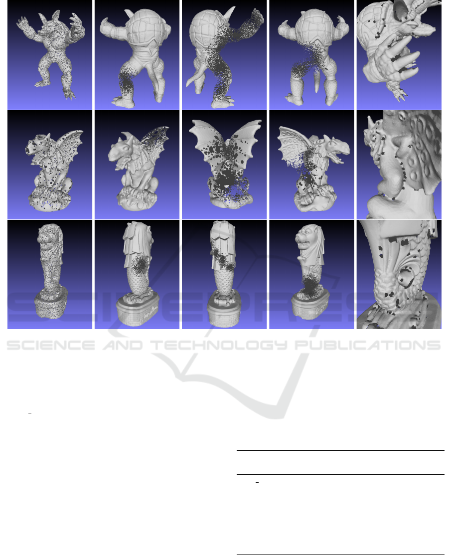
(a) Random (b) Cluster (c) Clusters set sepa-

rately

(d) Clusters set merged (e) Patch

Figure 5: Here, we present the results of topological noise generation applied to the armadillo, gargoyle, and Merlion meshes.

Each type of noise affects a different part of the mesh, as shown in the images. Random noise evenly covers the mesh with

holes. The cluster noise generates a single hole in the mesh, or a cascade of merged or separate holes. The patch noise

generates tiny holes at the bending points of the surface.

Kinect Fusion technique (Izadi et al., 2011). We eval-

uate the natural noise distribution by collecting shifts

of each node along its corresponding normal vector.

We use our library to generate artiﬁcial noise with

a Student distribution, with parameters n = 5 and

scale = 0.6. We collect the shift values of our arti-

ﬁcial noise for all meshes and calculate the KL diver-

gence and Chi-squared distance between the artiﬁcial

distribution and the Microsoft Kinect v1 distribution.

The results are 0.007 and 0.006, respectively. We also

calculate the KL divergence and Chi-squared distance

between each individual mesh’s natural noise and the

total natural noise, for comparison. The total natu-

ral and total artiﬁcial noise distributions are shown

in Figure 6. We calculate the distances between the

natural noise distributions of the mesh and the mean

artiﬁcial/natural distribution. The mean is calculated

over all ﬁgures considered. The results are presented

in Table 2.

Table 2: Each column contains the distance from speciﬁed

mesh natural noise distribution and average artiﬁcial or av-

erage natural distributions. KL divergence and Chi-squared

distance are used as measures.

Mesh

KL nat.

×10

−3

KL art.

×10

−3

Chi sq.

nat.

Chi sq.

art.

big girl 132 167 113 135

boy01 22 36 18 30

boy02 63 81 41 46

cone 100 100 95 94

david 58 56 22 21

girl 23 36 24 36

pyramid 56 59 47 49

The total distribution histogram is close to the Stu-

dent distribution. Each mesh natural noise distribu-

tion separately differs from the artiﬁcial distribution

approximately the same. The total natural noise dis-

tribution differs signiﬁcantly from the artiﬁcial one

VISAPP 2025 - 20th International Conference on Computer Vision Theory and Applications

672

Figure 6: Comparison of artiﬁcial Student distribution (n =

5) noise with natural noise of Microsoft Kinect v1. The

distributions are close.

compared to any separate natural distribution from the

total natural noise distribution.

6 MESH DENOISING PROBING

In this section, we demonstrate the denoising meth-

ods applied to dataset generated by our library. Some

learning-based denoising algorithms were also trained

on this dataset.

The following methods are used for noise re-

moval: Bilateral normal ﬁltering (C.-L., 2011),

Guided bilateral normal ﬁltering (Zhang W., 2015),

Fast and effective feature preserving mesh denois-

ing (Sun X, 2007), GeoBi-GNN (Zhang Y., 2022),

Cascaded normal regression (Wang P.-S., 2016).

Learning-based methods were trained on the Syn-

thetic data of dataset from (Wang P.-S., 2016).

For the evaluation of selected methods on gener-

ated node noise data, we choose the following met-

rics:

• Average weighted Hausdorff distance:

Err

∑

∈V

min

∈

(||v

−v

||), (5)

where N

is the number of vertices in the ground

truth mesh, L

is the length of the noisy mesh min-

imal oriented bounding box diagonal, V and

V are

an original and noisy mesh vertices’ sets respec-

tively.

• Average normal angular difference between

ground truth and denoised meshes:

Err

Ang

∑

∈F

arccos(n

), (6)

Table 3: Complicated geometry models denoising metrics.

Method

Hausdorff

×10

−3

Angle

×10

−4

Bilateral 0.67 8.79 2.96

Guided mesh 0.70 10.09 3.19

Fast and Effective 1.28 13.99 10.8

GeoBi-GNN 0.55 5.04 1.93

Cascaded 0.55 6.86 2.06

Table 4: CAD models denoising metrics.

Method

Hausdorff

×10

−3

Angle

×10

−4

Bilateral 1.20 2.29 1.73

Guided mesh 1.21 2.53 1.79

Fast and Effective 1.28 2.64 2.0

GeoBi-GNN 1.17 2.56 1.77

Cascaded 1.16 2.12 1.66

where F is a set of mesh faces, N

is F cardinality,

and

are normals of the same face of ground

truth and noisy mesh respectively.

• Average Chamfer Distance:

Err

|V |

−1



∑

∈V

∥v

−argmin

∈

∥v

−v

∥)∥

∑

∈

∥v

−argmin

∈V

∥v

−v

∥)∥

(7)

These metrics are borrowed from (Shen Y.,

2022), (Zhang W., 2015). The result metrics of de-

noising probing are presented in tables 3, 4 and 5. The

detailed table is provided in supplementary materials

in our GitHub repository.

Each metric is obtained by averaging over all de-

noised meshes, regardless of the type of noise. These

denoising metrics are comparable to those that can be

achieved in tests using Kinect Fusion. The normal

angular difference ranges from approximately 0.5 to

3.6 degrees, depending on the ﬁgure, and the Chamfer

distance ranges from 0.1 to 0.3 ×10

−4

. These values

are quoted from (Mashurov and Semenova, 2024).

7 CONCLUSION AND FUTURE

WORK

In this paper, we present a new library for generating

mesh noise. The library includes node and topologi-

cal noise generation methods, with a total of 15 meth-

ods implemented. Each algorithm can be adjusted us-

ing a set of input parameters, depending on the user’s

requirements.

Noisemaker 3D: Comprehensive Framework for Mesh Noise Generation

673

Table 5: Smooth surface models denoising metrics.

Method

Hausdorff

×10

−3

Angle

×10

−4

Bilateral 1.24 3.9 6.94

Guided mesh 1.31 5.27 7.93

Fast and Effective 2.09 6.3 17.6

GeoBi-GNN 1.16 2.7 5.67

Cascaded 1.12 3.17 5.67

The algorithms have been tested on a synthetic

dataset, using ﬁve non-learning and learning-based

denoising methods. Tables with the resulting met-

rics are provided. The experiments demonstrate that

meshes with artiﬁcial noise generated using our tool

can be effectively denoised. The denoising metrics

achieved in our tests are of the same order, and some-

times almost equal, as those in Kinect Fusion tests.

Currently, the parameters for topological noise

generation are not automatically adjusted. In future

work, these algorithms will automatically select input

parameters based on model size and speciﬁc require-

ments. Moreover, we will examine the meshes gen-

erated with topological noise on existing hole-ﬁlling

algorithms. We will perform an objective comparison

with the noise from real 3D sensors. For this purpose,

we will use Kinect to collect a dataset.

REFERENCES

Botsch J., Jain H., H. O. (2022). Imd-net: A deep learning-

based icosahedral mesh denoising network. IEEE Ac-

cess, 10:38635–38649.

C.-L., Z. Y. F. H. A. O. K.-C. T. (2011). Bilateral normal

ﬁltering for mesh denoising. IEEE Transactions on

Visualization and Computer Graphics, 17(10):1521–

1530.

Dai A., Qi C.R., N. M. (2017). Shape Completion Using

3D-Encoder-Predictor CNNs and Shape Synthesis. In

Proceedings of the IEEE Conference on Computer Vi-

sion and Pattern Recognition (CVPR), pages 5868–

5877, Honolulu, Hawaii, USA. IEEE.

Davis J., Marschner S.R., G. M. L. M. (2002). Fill-

ing holes in complex surfaces using volumetric diffu-

sion. In Proceedings. First International Symposium

on 3D Data Processing Visualization and Transmis-

sion, pages 428–441, Padua, Italy. IEEE.

I., Y. Y. P. N. I. (2013). Linear correlations between

spatial and normal noise in triangle meshes. IEEE

Transactions on Visualization and Computer Graph-

ics, 19(1):45–55.

Izadi, S., Kim, D., Hilliges, O., Molyneaux, D., Newcombe,

R., Kohli, P., Shotton, J., Hodges, S., Freeman, D.,

Davison, A., et al. (2011). Kinectfusion: real-time 3d

reconstruction and interaction using a moving depth

camera. In Proceedings of the 24th annual ACM sym-

posium on User interface software and technology,

pages 559–568.

Kamberova G., B. R. (1997). Precision of 3D points recon-

structed from stereo. Technical Report . MS-CIS-97-

20, Dept. of Computer & Information Science, Univ.

of Pennsylvania.

Litany O., Bronstein A., B. M. M. A. (2018). Deformable

Shape Completion With Graph Convolutional Au-

toencoders. In Proceedings of the IEEE Conference

on Computer Vision and Pattern Recognition (CVPR),

pages 1886–1895, Salt Lake City, Utah, USA. IEEE.

Ma Z., L. S. (2018). A review of 3d reconstruction tech-

niques in civil engineering and their applications. Ad-

vanced Engineering Informatics, 37:163–174.

Mashurov, V. and Semenova, N. (2024). Topological and

node noise ﬁltering on 3d meshes using graph neu-

ral networks (student abstract). In Proceedings of

the AAAI Conference on Artiﬁcial Intelligence, vol-

ume 38, pages 23582–23584.

Nguyen C. V., Izadi S., L. D. (2012). Modeling Kinect

Sensor Noise for Improved 3D Reconstruction and

Tracking. In 2012 Second International Conference

on 3D Imaging, Modeling, Processing, Visualization

& Transmission, pages 524–530, Zurich, Switzerland.

IEEE.

Shen Y., Fu H., D. Z. C. X. B. E.-Z. D. Z. K. Z. Y. (2022).

Gcn-denoiser: Mesh denoising with graph convolu-

tional networks. ACM Transactions on Graphics,

41(1):1—-14.

Sun X, Rosin P. L., M. R. L. F. (2007). Fast and ef-

fective feature-preserving mesh denoising. IEEE

Transactions on Visualization and Computer Graph-

ics, 13(5):925–938.

Wang P.-S., Liu Y., T. X. (2016). Mesh denoising via

cascaded normal regression. ACM Transactions on

Graphics, 35(6):1–12.

Yadav S.K., Reitebuch U., S. M. Z. E. P. K. (2018).

Constraint-based point set denoising using normal

voting tensor and restricted quadratic error metrics.

Computers & Graphics, 74:234—-243.

Zhang W., Deng B., Z. J. B. S. L. L. (2015). Guided mesh

normal ﬁltering. Comput. Graph. Forum., 34(7):23–

–34.

Zhang Y., Shen G., W. Q. Q. Y. W. M.-Q. J. (2022).

Geobi-gnn: Geometry-aware bi-domain mesh denois-

ing via graph neural networks. Computer-Aided De-

sign, 144:103154.

Zhao W., Liu X., Z. Y. F. X. Z. D. (2021). Normal-

net: Learning-based mesh normal denoising via local

partition normalization. IEEE Transactions on Cir-

cuits and Systems for Video Technology, 31(12):4697–

4710.

Zhong M., Q. H. (2016). Surface inpainting with spar-

sity constraints. Computer Aided Geometric Design,

41:23–35.

VISAPP 2025 - 20th International Conference on Computer Vision Theory and Applications

674