A Discrete Non-Additive Integral Based Interval-Valued Neural Network
for Enhanced Prediction Reliability
Yassine Hmidy and Mouna Ben Mabrouk
Sogetilabs at Capgemini, Paris, France
Keywords:
Neural Networks, Regression, Interval-Valued, Aggregation Function, Trustworthiness.
Abstract:
In this paper, we propose to replace the perceptron of classical feedforward neural networks by a new aggre-
gation function. In a recent paper, it has been shown that this new aggregation is a relevant learning model,
simple to use, and informative as it outputs an interval whose size is correlated to the prediction error of the
model. Unlike a classical neural network whose perceptron are usually composed of a linear aggregation and
an activation function, the model we propose here is a mere composition of those aggregation functions. In or-
der to show the relevance of using such a neural network, we rely on experiments comparing its performances
with those of a classical neural network.
1 INTRODUCTION
An aggregation function is by definition any function
that computes a single output value from a vector of
input values. Among these, there are parametric ag-
gregation functions whose computation involves op-
erations between a vector of parameters and the vec-
tor of input values. The most commonly used in ma-
chine learning model is the arithmetic mean. It is the
core operation of each perceptron in classical neural
networks.
Though a wide range of activation functions
have been customized, from sigmoid functions to
ReLU functions, the arithmetic mean still remains un-
changed in most of the current neural network. In
this paper, we propose a conceptual breakthrough,
not only by changing the arithmetic mean for another
parametric aggregation function, but by changing the
total perceptron. The new perceptron we propose is
based on a parametric aggregation function named the
Macsum aggregation (Strauss et al., 2022). The Mac-
sum aggregation outputs an interval whose bounds
are discrete Choquet integrals. The learning abilities
of the Macsum aggregation is presented in (Hmidy
et al., 2022b). In this paper we build a neural net-
work whose neurons computes the center of Macsum
aggregations except for the last neuron which com-
putes a Macsum aggregation. Therefore the output is
interval-valued. In (Hmidy et al., 2022b), the corre-
lation between the width of the interval-valued output
of the Macsum aggregation and the prediction error
made by the model has been demonstrated. An ex-
periment we carried on demonstrated that the neural
network we propose keeps this property.
In summary, the paper contribution is three fold:
• a new learning model, that is a neural network
whose perceptrons compute discrete Choquet in-
tegrals based aggregation functions,
• the possibility to assess the trustworthiness of a
prediction comparing to another through the size
of its interval-valued output,
• the unnecessity of using activation functions
thanks to the non-linearity naturally induced by
the composition of Macsum aggregations.
2 RELATED WORK
In this section we situate our work w.r.t. the literature.
2.1 Choquet Integral Based Neural
Network
The Choquet integral is a generalization of Lebesgue
integral to non-additive measures (Grabisch, 2015).
It is commonly used in decision theory to account for
situations that cannot be represented by additive set
functions (or games). The relevance of using a Cho-
quet integral as a neuron in a neural network imple-
mentation for decision analysis is presented in (Chi-
ang, 1999). In (Shi-Hong and Zheng-You, 2005), a
Hmidy, Y. and Ben Mabrouk, M.
A Discrete Non-Additive Integral Based Interval-Valued Neural Network for Enhanced Prediction Reliability.
DOI: 10.5220/0013155900003890
Paper published under CC license (CC BY-NC-ND 4.0)
In Proceedings of the 17th International Conference on Agents and Artificial Intelligence (ICAART 2025) - Volume 2, pages 345-352
ISBN: 978-989-758-737-5; ISSN: 2184-433X
Proceedings Copyright © 2025 by SCITEPRESS – Science and Technology Publications, Lda.
345

Choquet integral-based neural network turned out to
be efficient in multi-classification tasks. In (Machado
et al., 2015), the use of a bipolar Choquet integral led
to promising results for classification in a context of
decision making where underlying scales are bipolar.
More recently, in (Bresson et al., 2020), a neural rep-
resentation of a hierarchical 2-additive Choquet inte-
gral has shown efficiency in classification, regression
and ranking settings .
2.2 Interval Neural Network
An interval neural network is a neural network whose
output is interval-valued.
The interval-valued nature of the output can be
due to the use of interval parameters (Garczarczy,
2000; Oala et al., 2020; Beheshti et al., 1998). In
these architectures the forward propagation is ex-
pressed similarly to classical neural networks by us-
ing interval arithmetic instead of usual arithmetic.
This interval-valued nature can also be induced
by considering a neural network with interval-valued
inputs. Many neural networks have been extended
to learn from interval-valued inputs. In (Rossi and
Conan-Guez, 2002; Kowalski and Kulczycki, 2017),
a probabilistic neural network allows to learn from
interval-valued data considering an interval as a uni-
form distribution between two bounds. We can also
find in the literature extension of neural networks to
fuzzy input vectors (Hisao and Manabu, 2000).
2.3 Prediction Intervals
Neural networks are used in prediction tasks due to
their strong performance and flexibility in modeling
complex functions. With the increasing use of neu-
ral networks comes the need for developing tools to
estimate the uncertainty of their predictions. Predic-
tion intervals is a way to give a measure of uncer-
tainty that can be used on regression problems. Many
techniques exist to build such an interval in the case
of neural networks. For instance, in (Khosravi et al.,
2014), the bootstrap approach (Efron, 1979) is used to
build prediction intervals of the neural network out-
puts. In (Mancini et al., 2021) is presented another
method that consists in building multiple neural net-
work models and use their outputs to build the predic-
tion interval.
In this paper we present a feedforward neural net-
work based on a Choquet integral w.r.t. a parametric
set function. This neural network outputs an interval
that can be considered as an error prediction.
3 PRELIMINARIES
3.1 Notations and Definitions
• Ω = {1,...,N} ⊂ .
• ∀A ⊆ Ω, A
c
is the complementary of A in Ω.
• is the set of real numbers.
• A vector is a function x : Ω → defined by a dis-
crete subset of denoted x = (x
1
,··· ,x
N
) ∈ .
• x = [x,x] is a real interval whose lower bound is
x ∈ and upper bound is x ∈ .
• is the set of real intervals.
• A set function is a function µ : 2
Ω
→ that maps
any subset of Ω onto a real value. To a set function
µ is associated its complementary set function µ
c
:
∀A ⊆ Ω, µ
c
(A) = µ(Ω)−µ(A
c
). Usually, µ(
/
0) = 0
where
/
0 is the emptyset of Ω.
• A set function µ is said to be submodular if
∀A,B ⊆ Ω, µ(A ∪ B) + µ(A ∩ B) ≤ µ(A) + µ(B).
• A set function µ is said to be additive if ∀A,B ⊆ Ω,
µ(A ∪ B) + µ(A ∩ B) = µ(A) + µ(B).
• If a set function µ is submodular then its comple-
mentary µ
c
is supermodular.
• The discrete Choquet integral w.r.t. a set function
µ is denoted
ˇ
µ
(Grabisch et al., 2000) and
defined by :
ˇ
µ
(x) =
N
∑
k=1
x
(k)
.(µ(A
(k)
) − µ(A
(k+1)
)). (1)
(.) being the permutation that sorts the element
of x in increasing order: x
(1)
≤ x
(2)
≤ ··· ≤ x
(N)
and A
(i)
(i ∈ Ω) being the coalition of Ω such that
A
(i)
= {(i),.. ., (N)} with A
(N+1)
=
/
0.
• If a set function µ is submodular then ∀x ∈
N
,
ˇ
µ
(x) ≥
ˇ
µ
c
(x) (Grabisch, 2016).
3.2 Macsum Aggregation
Let θ ∈
N
be a vector used as a parameter. The Mac-
sum set function ν
θ
and its complementary set func-
tion ν
c
θ
, has been defined in (Strauss et al., 2022) as
∀A ⊆ Ω:
ν
θ
(A) = max
i∈A
θ
+
i
+ min
i∈Ω
θ
−
i
− min
i∈A
c
θ
−
i
, (2)
ν
c
θ
(A) = min
i∈A
θ
−
i
+ max
i∈Ω
θ
+
i
− max
i∈A
c
θ
+
i
, (3)
with ∀i ∈ Ω, θ
+
i
= max(0,θ
i
) and θ
−
i
= min(0,θ
i
).
ICAART 2025 - 17th International Conference on Agents and Artificial Intelligence
346

The Macsum set function being a parametric set
function that is submodular (Strauss et al., 2022),
ˇ
ν
θ
(x) ≥
ˇ
ν
c
θ
(x). The Macsum aggregation A
ν
θ
is
defined by using the Macsum set function such that:
∀x ∈
N
, y = [y,y] = A
ν
θ
(x) = [
ˇ
ν
c
θ
(x),
ˇ
ν
θ
(x)].
Let ψ ∈
N
, ∀A ⊆ Ω, we denote λ
ψ
the linear
parametric set function defined by:
λ
ψ
(A) =
∑
i∈A
ψ
i
.
A consequence of the submodularity of the Macsum
set function is that it dominates a set of linear para-
metric set function (Strauss et al., 2022).
The set of all parameters ψ such that λ
ψ
is domi-
nated by the Macsum set function w.r.t. the parameter
θ can be written this way:
M (θ) = {ψ ∈
N
|∀A ⊆ Ω,ν
c
θ
(A) ≤ λ
ψ
(A) ≤ ν
θ
(A)}.
This set is convex (Strauss et al., 2022), which
means that ∀ψ
1
,ψ
2
∈ M (θ),γψ
1
+(1−γ)ψ
2
∈ M (θ)
with γ ∈ [0,1].
Let ψ ∈
N
, the linear aggregation is defined by
using the linear operator λ
ψ
as:
A
λ
ψ
(x) =
ˇ
λ
ψ
(x) =
∑
i∈Ω
ψ
i
.x
i
.
Therefore, the Macsum aggregation can be inter-
preted as:
A
ν
θ
(x) =
n
A
λ
ψ
(x)/ψ ∈ M (θ)
o
= [A
ν
θ
(x),A
ν
θ
(x)], (4)
this set being convex (Strauss et al., 2022): ∀ψ ∈
M (θ), ∃y ∈ A
ν
θ
(x) such that y = A
λ
ψ
(x) and ∀y ∈
A
ν
θ
(x), ∃ψ ∈ M (θ) such that y = A
λ
ψ
(x).
As the Macsum aggregation is a set of linear
aggregation whose bounds depend on the same pa-
rameter, we can learn a set of linear aggregation by
learning a Macsum aggregation through the updat-
ing of one parameter, with the usual gradient descent
method as shown in (Hmidy et al., 2022b).
3.3 Computation of the Macsum
Aggregation
The upper and lower bound of the Macsum aggrega-
tion of a vector x ∈
N
w.r.t. a parameter θ ∈
N
can
easily be obtained by considering expressions (1), (2)
and (3):
A
ν
θ
(x) =
N
∑
k=1
x
(k)
.

N
max
i=k
θ
+
(i)
−
k−1
min
i=1
θ
−
(i)

−
N
∑
k=1
x
(k)
.

N
max
i=k+1
θ
+
(i)
+
k
min
i=1
θ
−
(i)

, (5)
and
A
ν
θ
(x) =
N
∑
k=1
x
(k)
.

N
min
i=k
θ
−
(i)
−
k−1
max
i=1
θ
+
(i)

−
N
∑
k=1
x
(k)
.

N
min
i=k+1
θ
−
(i)
+
k
max
i=1
θ
+
(i)

, (6)
where (.) is the permutation that sorts the element of
x in increasing order: x
(1)
≤ x
(2)
≤ ··· ≤ x
(N)
.
There exists an equivalent form for the Macsum
aggregation (Hmidy et al., 2022b) allowing its com-
putation with sorting the parameter vector θ instead
of sorting the input vector x:
A
ν
θ
(x) =
N
∑
k=1
θ
+
⌊k⌋
.

k
max
i=1
x
⌊i⌋
−
k−1
max
i=1
x
⌊i⌋

+
N
∑
k=1
θ
−
⌈k⌉
.

k
min
i=1
x
⌈k⌉
−
k−1
min
i=1
x
⌈k−1⌉

, (7)
and:
A
ν
θ
(x) =
N
∑
k=1
θ
−
⌊k⌋
.

k
min
i=1
x
⌊i⌋
−
k−1
min
i=1
x
⌊i⌋

+
N
∑
k=1
θ
+
⌈k⌉
.

k
max
i=1
x
⌈k⌉
−
k−1
max
i=1
x
⌈k−1⌉

, (8)
where ⌊.⌋ is a permutation that sorts θ in de-
creasing order (θ
⌊1⌋
≥ θ
⌊2⌋
≥ ··· ≥ θ
⌊N⌋
), and ⌈.⌉
is a permutation that sorts θ in increasing order
(θ
⌈1⌉
≤ θ
⌈2⌉
≤ · ·· ≤ θ
⌈N⌉
), with min
0
i=1
x
⌊i⌋
= 0 =
max
0
i=1
x
⌈i⌉
andmax
0
i=1
x
⌊i⌋
= 0 = min
0
i=1
x
⌈i⌉
.
4 MACSUM NEURAL NETWORK
FOR REGRESSION
In this section, we present a new learning model based
on the Macsum aggregation to replace the classical
neuron in a feedforward neural network. The mo-
tivation for introducing this model is to show that
the flexibility of the aggregation function we propose
can model a wide range of input/output relations and
therefore allows to get rid of the activation function
whose choice is often arbitrary. We define the Mac-
sum perceptron as being the center of the Macsum
aggregation. Getting rid of the activation function
is possible thanks to the inherent non-linearity of the
Macsum perceptron.
4.1 Macsum Perceptron
We propose to define the Macsum perceptron, de-
noted S
ν
θ
, as being the following parametric function:
A Discrete Non-Additive Integral Based Interval-Valued Neural Network for Enhanced Prediction Reliability
347

∀θ ∈
N
, S
ν
θ
:
N
→
x 7→
1
2

A
ν
θ
(x) + A
ν
θ
(x)

As for any classical perceptron, the learning
process of a Macsum perceptron uses the gradient
descent method to update the parameters. To able
a similar learning process, the derivatives of the
Macsum perceptron w.r.t. its parameters and w.r.t. its
inputs are required.
The derivative of A
ν
θ
and A
ν
θ
w.r.t. its parame-
ters have been established in (Hmidy et al., 2022b) .
The derivative of S
ν
θ
w.r.t. the k
th
parameter is:
δS
ν
θ
(x)
δθ
k
=
1
2
.

l
max
i=1
x
⌊i⌋
−
l−1
max
i=1
x
⌊i⌋
+
u
min
i=1
x
⌈i⌉
−
u−1
min
i=1
x
⌈i⌉
+
l
min
i=1
x
⌊i⌋
−
l−1
min
i=1
x
⌊i⌋
+
u
max
i=1
x
⌈i⌉
−
u−1
max
i=1
x
⌈i⌉

,
with l and u being the index such that ⌊l⌋ = k and
⌈u⌉ = k.
The derivates of S
ν
θ
(x) w.r.t. its inputs can be
easily obtained by considering Equations (5) and (6):
δS
ν
θ
(x)
δx
k
=
1
2
.

N
max
i=l
θ
+
(i)
−
l−1
min
i=1
θ
−
(i)
−
N
max
i=l+1
θ
+
(i)
+
l
min
i=1
θ
−
(i)
+
N
min
i=l
θ
−
(i)
−
l−1
max
i=1
θ
+
(i)
−
N
min
i=l+1
θ
−
(i)
+
l
max
i=1
θ
+
(i)

,
with (.) being the permutation that sorts the element
of x in increasing order: x
(1)
≤ x
(2)
≤ · ·· ≤ x
(N)
and
l the index such that (l) = k.
4.2 A Non-Linear Model with no
Activation Function
In a classical feedforward neural network each per-
ceptron is composed of a linear aggregation function
followed by an activation function. In the case of a
Macsum neural network the aggregation function is
non-linear which rids the model of activation func-
tions. Let us give a simple example:
Let θ = (−1, 2,−3), x = (1,0, 3) and y = (−2, 3,9):
then S
ν
θ
(x + y) = 4 while S
ν
θ
(x) + S
ν
θ
(y) = 5.
Consequently, each perceptron of a Macsum neu-
ral network is non-linear as for a classical neural net-
work.
4.3 An Interval Model for Regression
A way to learn the parameters of a Macsum aggre-
gation based on a dataset have been proposed in
(Hmidy et al., 2022b). The experiment associated
to this work shed light on a correlation between the
width of the interval-valued output and the prediction
error, i.e. the distance between the target value and
the center of the interval-valued output. This property
is interesting since it allows to have information on
the quality of a prediction. We propose to keep this
prediction ability by using a Macsum aggregation
instead of a Macsum perceptron for the last neuron.
This will provide an interval valued output. The
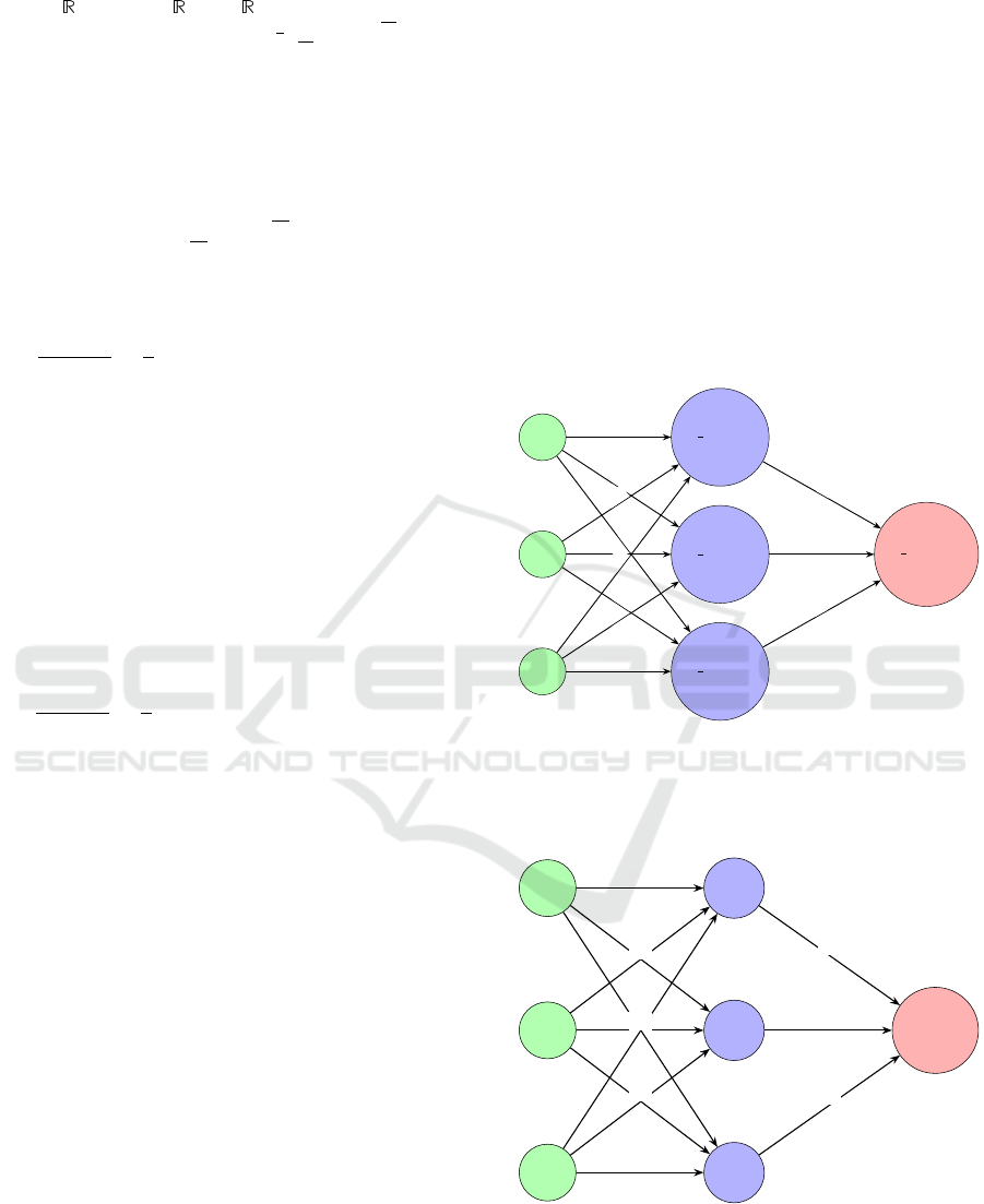
idea is to change this classical structure: To obtain
Input
I
1
Input
I
2
Input
I
3
σ

1
3
3
P
i=1
w
(1)
i1
I
i

σ

1
3
3
P
i=1
w
(1)
i2
I
i

σ

1
3
3
P
i=1
w
(1)
i3
I
i

σ

1
3
3
P
j=1
w
(2)
j
H
j

w
(1)
11
w
(1)
12
w
(1)
13
w
(1)
21
w
(1)
22
w
(1)
23
w
(1)
31
w
(1)
32
w
(1)
33
w
1
w
2
w
3
Figure 1: Classical neural network.
a structure in which neuron on the hidden layers are
Macsum perceptron and the output neuron is the
Macsum aggreation and is therefore interval-valued.
Input
I
1
Input
I
2
Input
I
3
S
ν
θ
1
(x)
S
ν
θ
2
(x)
S
ν
θ
3
(x)
A
ν
(2)
θ
(x
(2)
)
θ
(1)
11
θ
(1)
12
θ
(1)
13
θ
(1)
21
θ
(1)
22
θ
(1)
23
θ
(1)
31
θ
(1)
32
θ
(1)
33
θ
(2)
1
θ
(2)
2
θ
(2)
3
Figure 2: Macsum neural network.
ICAART 2025 - 17th International Conference on Agents and Artificial Intelligence
348

5 EXPERIMENTS
We present two experiments. The aim of the first ex-
periment was to show the relevance of using a Mac-
sum neural network as a learning model compared to
a Macsum aggregation. The aim of the second ex-
periment was to demonstrate the ability of a Macsum
neural network to compete with a classical neural net-
work on a regression task.
To determine the performances of a learning
model we relied on the following criteria:
• the cost value which is the Euclidean distance be-
tween the middle of the predicted output
1
2
(y + y)
and the actual output (target) for the Macsum neu-
ral network and the Euclidean distance between
the predicted output and the actual output for the
classical networks,
• the resulting criterion R
2
(Lewis-Beck, 2015),
• the belonging rate that is the percentage of targets
that belongs to the interval-valued output [y, y],
• the mean width of the predicted output
1
2
(y − y)
for the Macsum neural network,
• the Pearson correlation between the predicted er-
ror
1
2
(y − y) and the prediction error for the Mac-
sum neural network.
5.1 Comparison with a Macsum
Aggregation
In these experiments we first compared a Macsum
neural network to a Macsum aggregation on their abil-
ity to learn a linear relation. Secondly, we compared
them on their ability to learn a non-linear relation in
order to shed light on the relevance of using a Mac-
sum neural network instead of a simple Macsum ag-
gregation.
We implemented these experiment on noiseless
synthetic data.
We built two dataset of 700 examples such that
∀i ∈ {1,...,700} the i
th
target was a real value
y
i
= f (X
i
,ψ) with the parameter ψ ∈
13
randomly
picked according to the standard normal distribution
and the elements of the input vectors X
i
∈
13
were
uniformly picked between −10 and 10.
The function f was linear in the first experiment and
non-linear in the second.
We split the dataset into 500 examples for the
training phase and 200 examples for the test phase.
To perform these experiments, we proposed to use
a very simple fully connected 3-layer neural network
with two neurons on the input layer, two neurons on
the hidden layer and one neuron on the output layer.
The learning rate was arbitrarily set to 0.001 and
the number of epochs to 2000.
5.1.1 Learning a Linear Relation
The linear relation had the following form:
∀i ∈ {1,...,700}, y
i
=
∑
13
j=1
X
i
j
.ψ
j
.
Table 1: Results on the linear dataset.
Criteria Macsum Net Macsum Neuron
train / test train / test
Cost value 0.33 / 0.43 0.24 / 0.57
Belonging 80.3% / 80.3% 100% / 100%
Width 6.34 / 6.04 652 / 703
R
2
0.992 / 0.992 1 / 1
Table 1 brought out the ability of the Macsum neu-
ral network to learn linear data since the cost value
was quite low and R
2
was high. Nevertheless the
Macsum perceptron outperformed it in terms of be-
longing rate. Although the Macsum neural network
gave much smaller intervals than the Macsum aggre-
gation. Thus, the interval-valued output given by the
Macsum neural network was much more informative
than this of the Macsum aggregation.
Furthermore, the similarity of the performances
on both the train and the test dataset showed the gen-
eralization ability of both models.
5.1.2 Learning a Non-Linear Relation
As the Macsum aggregation is a convex set of linear
functions, the aim here was to show that a composi-
tion of Macsum perceptron was non-linear enough to
get rid of activation functions.
The non-linear relation had the following form:
∀i ∈ {1,...,700}, y
i
=
∑
13
j=1
sin(X
i
j
).ψ
j
.
We chose a sinusoidal function because of its
strong non-linearity.
Table 2: Results on the non-linear dataset.
Criteria Macsum Net Macsum Neuron
train / test train / test
Cost value 12.27 / 9.36 52.09 / 55.36
Belonging 52% / 50.9% 49.6% / 49.6%
Width 7.31 / 8.35 18.52 / 18.30
R
2
0.94 / 0.95 0.053 / 0.029
In Table 2, the significant difference between the
R
2
of the Macsum neural network and the Macsum
perceptron showed the relevance of using a network
of Macsum perceptron instead of a simple Macsum
perceptron to learn non-linear relations. As in the
previous experiment, the neural network gave a more
A Discrete Non-Additive Integral Based Interval-Valued Neural Network for Enhanced Prediction Reliability
349

specific i.e. more informative interval. Also the R
2
was the same on both training and test dataset.
5.2 Comparison Between Macsum
Neural Network and Classical
Neural Network Across Multiple
Datasets
The goal of this experiment was to compare the per-
formance of a Macsum neural network with a clas-
sical neural network across multiple regression tasks
using different datasets. Each dataset involves pre-
dicting a variable based on others, with neural net-
works structured identically across tasks.
In all experiments, the networks were composed
of 8 fully connected layers (6 hidden layers) with 9
neurons in the first layer, 18 in the second, 36 in the
third, 72 in the fourth, 36 in the fifth, 18 in the sixth,
9 in the seventh, and 1 neuron in the last layer. This
structure was chosen arbitrarily for consistency across
datasets.
In a classical neural network, each neuron is com-
posed of an affine function (a linear aggregation with
a bias) and an activation function, except for the last
perceptron, which has no activation function. For the
Macsum neural network, each neuron is composed of
a Macsum perceptron, which is a non-linear aggrega-
tion function with no bias and no activation function.
The learning rate was initialized at 10
−12
for the
classical neural network and 10
−5
for the Macsum
neural network in all experiments. Learning rates
were decreased gradually in steps of 1000 iterations
to encourage convergence.
Below, we describe the datasets and the tasks, fol-
lowed by a comparison of results.
5.2.1 Datasets
• Dataset 1: CalCOFI Dataset (Oceanographic
Data) (Dane, 2018)
Objective: Predict water temperature based on
salinity.
Inputs: Water salinity and other environmental
factors.
Output: Water temperature.
Samples: 1000 (randomly selected for training
and testing).
• Dataset 2: Szeged Weather Data (Budincsevity,
2017)
Objective: Predict apparent temperature based on
humidity.
Inputs: Humidity and other weather-related vari-
ables.
Output: Apparent temperature.
Samples: 800 (randomly selected).
• Dataset 3: World War Two Weather Data
(Smith, 2019)
Objective: Predict maximum temperature based
on minimum temperature.
Inputs: Daily minimum temperature.
Output: Daily maximum temperature.
Samples: 700 (randomly selected).
• Dataset 4: Montreal Bike Lane Usage (Mon-
leon, 2020)
Objective: Predict the number of bicyclists on
a specific bike path based on counts from other
paths.
Inputs: Counts of bicyclists on different bike
paths.
Output: Number of bicyclists on a selected path.
Samples: 600 (randomly selected).
• Dataset 5: New York City East River Bicycle
Crossings (of New York, 2021)
Objective: Predict the number of bicyclists on one
bridge based on counts from other bridges.
Inputs: Counts of bicyclists on different bridges.
Output: Number of bicyclists on a specific
bridge.
Samples: 800 (randomly selected).
• Dataset 6: UK Road Safety Data (Tsiaras,
2020)
Objective: Predict the number of casualties in
road accidents based on the number of people in
the car.
Inputs: Number of people in the car and other
contextual factors.
Output: Number of casualties.
Samples: 900 (randomly selected).
5.3 Results Across Datasets
The following tables summarize the results of the ex-
periments on all datasets for both the Macsum neural
network and the classical neural network.
5.3.1 Euclidean Distance (Train/Test)
The classical neural network learning curve often
shows variability in the learning process depending
on the dataset used, with performance improvements
occurring at different rates and sometimes with sig-
nificant fluctuations. In contrast, with the Macsum
neural network, the learning process tends to be more
uniform across different datasets. This indicates that
Macsum networks may generalize better, with more
stable convergence patterns, reducing the impact of
ICAART 2025 - 17th International Conference on Agents and Artificial Intelligence
350

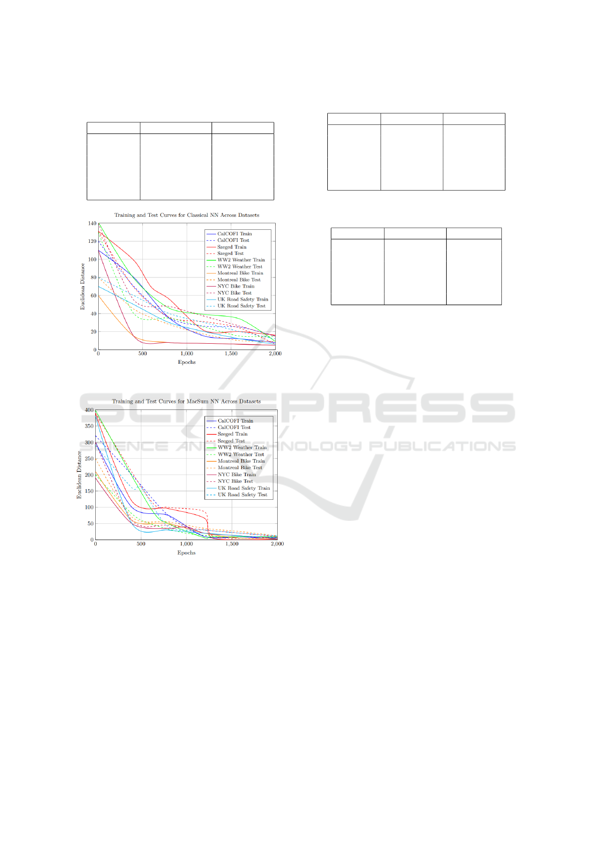
Table 3: Euclidean Distance across datasets for both mod-
els.
Dataset Classical NN Macsum NN
CalCOFI 12.532 / 13.145 6.314 / 6.765
Szeged 14.120 / 15.812 7.821 / 8.335
WW2 11.431 / 12.009 5.157 / 5.634
Mt. Bike 7.215 / 7.897 3.712 / 3.987
NYC Bike 8.635 / 9.324 4.012 / 4.563
UK Road 5.135 / 6.023 2.985 / 3.235
Figure 3: Euclidean Distance across datasets for the classi-
cal neural network.
Figure 4: Euclidean Distance across datasets for the Mac-
sum neural network.
dataset-specific characteristics on learning stability
and speed.
5.3.2 R
2
Coefficient (Train/Test)
5.3.3 Mean Width of Predicted Output
As seen in table 5, the correlation between the pre-
dicted and actual errors steadily increases with more
training epochs, indicating that both networks are be-
coming more capable of reducing their error margins.
Table 4: R
2
Coefficient across datasets for both models.
Dataset Classical NN Macsum NN
CalCOFI 0.121 / 0.223 0.102 / 0.245
Szeged 0.341 / 0.315 0.253 / 0.325
WW2 0.212 / 0.290 0.221 / 0.301
Mt. Bike 0.174 / 0.223 0.202 / 0.285
NYC Bike 0.153 / 0.211 0.235 / 0.301
UK Road 0.042 / 0.125 0.123 / 0.201
Table 5: Mean Width and Pearson correlation across
datasets.
Dataset Mean Width Correlation
CalCOFI 14.7 / 13.2 0.68
Szeged 5.41 / 5.32 0.73
WW2 4.91 / 5.10 0.72
Mt. Bike 16.1 / 16.05 0.80
NYC Bike 5.31 / 5.45 0.66
UK Road 14.72 / 14.85 0.85
6 CONCLUSION AND FUTURE
WORK
In this work, we proposed a neural network whose
perceptrons are based on a new aggregation method
called the Macsum aggregation. Given the Macsum
perceptron is non-linear there is no need for activa-
tion functions. A comparison with a classical neural
network with a ReLu activation function confirmed
the potential competitiveness of the Macsum neural
network with regard to the state of the art. On top of
that, the Macsum neural network goes toward the cur-
rent trend of trustworthy learning model. Indeed, as
the length of the interval-valued output is correlated to
the error made by the model we have information on
the quality of the prediction that can be crucial in de-
cision making. Therefore not only the Macsum neural
network has satisfying learning performances but also
it gives insights of the prediction error.
Yet, many improvement can be done for increasing
the performances of the Macsum neural network. An
important issue to tackle is the computation cost of
the Macsum perceptron since it is much higher that
this of a classical perceptron. We could also think
of an architecture that combines Macsum perceptrons
with classical perceptrons to alleviate the computa-
tion cost. Further work could go towards trying to
tighten the size of the interval output for them to be
more informative. The potential of this new model
is far from being fully exploited and several direc-
tions might lead to interesting results. For instance
we could use an extension of the Macsum aggrega-
tion to interval-valued input (Hmidy et al., 2022a) to
learn from interval-valued data.
A Discrete Non-Additive Integral Based Interval-Valued Neural Network for Enhanced Prediction Reliability
351

REFERENCES
Beheshti, M., Berrached, A., de Korvin, A., Hu, C., and
Sirisaengtaksin, O. (1998). On interval weighted
three-layer neural networks. In Proceedings of the
31st Annual Simulation Symposium, pages 188–194.
Bresson, R., Cohen, J., H
¨
ullermeier, E., Labreuche, C., and
Sebag, M. (2020). Neural representation and learning
of hierarchical 2-additive choquet integrals. In Pro-
ceedings of the International Joint Conference on Ar-
tificial Intelligence (IJCAI), pages 1984–1991.
Budincsevity, N. (2017). Weather in szeged 2006-
2016. https://www.kaggle.com/datasets/budincsevity/
szeged-weather. Kaggle Dataset.
Chiang, J. (1999). Choquet fuzzy integral-based hierarchi-
cal networks for decision analysis. IEEE Transactions
on Fuzzy Systems, 7(1):63–71.
Dane, S. (2018). Calcofi. https://www.kaggle.com/datasets/
sohier/calcofi. Kaggle Dataset.
Efron, B. (1979). Bootstrap methods: Another look at the
jackknife. The Annals of Statistics, 7:1–26.
Garczarczy, Z. A. (2000). Interval neural networks. In 2000
IEEE International Symposium on Circuits and Sys-
tems (ISCAS), volume 3, pages 567–570.
Grabisch, M. (2015). Fuzzy measures and integrals: Recent
developments. In Fifty Years of Fuzzy Logic and Its
Applications, pages 125–151.
Grabisch, M. (2016). Set Functions, Games and Capacities
in Decision Making. Springer.
Grabisch, M., Sugeno, M., and Murofushi, T. (2000). Fuzzy
Measures and Integrals: Theory and Applications.
Physica, Heidelberg.
Hisao, I. and Manabu, N. (2000). Neural networks
for soft decision making. Fuzzy Sets and Systems,
115(1):121–140.
Hmidy, Y., Rico, A., and Strauss, O. (2022a). Extend-
ing the macsum aggregation to interval-valued inputs.
In 15th International Conference on Scalable Uncer-
tainty Management, volume 13562, pages 338–347.
Hmidy, Y., Rico, A., and Strauss, O. (2022b). Macsum ag-
gregation learning. Fuzzy Sets and Systems, 24.
Khosravi, A., Nahavandi, S., Srinivasan, D., and Khosravi,
R. (2014). Constructing optimal prediction intervals
by using neural networks and bootstrap method. IEEE
Transactions on Neural Networks and Learning Sys-
tems, 26:1810–1815.
Kowalski, P. A. and Kulczycki, P. (2017). Interval proba-
bilistic neural network. Neural Computing and Appli-
cations, 28.
Lewis-Beck, C. (2015). Applied Regression: An Introduc-
tion, volume 22. Sage Publications.
Machado, M., Flavio, L., Jusan, D., and Caldeira, A.
(2015). Using a bipolar choquet neural network to
locate a retail store. In 3rd International Conference
on Information Technology and Quantitative Manage-
ment, volume 55, pages 741–747.
Mancini, T., Calvo-Pardo, H., and Olmo, J. (2021). Predic-
tion intervals for deep neural networks. arXiv preprint
arXiv:2010.04044v2.
Monleon, P. (2020). Montreal bike lanes.
https://www.kaggle.com/datasets/pablomonleon/
montreal-bike-lanes. Kaggle Dataset.
Oala, L., Heiß, C., Macdonald, J., M
¨
arz, M., Samek, W.,
and Kutyniok, G. (2020). Interval neural networks:
Uncertainty scores. arXiv preprint arXiv:2003.11566.
of New York, C. (2021). New york city - east river
bicycle crossings. https://www.kaggle.com/datasets/
new-york-city/nyc-east-river-bicycle-crossings. Kag-
gle Dataset.
Rossi, F. and Conan-Guez, B. (2002). Multi-layer percep-
tron on interval data. In Classification, Clustering,
and Data Analysis, pages 427–434.
Shi-Hong, Y. and Zheng-You, W. (2005). Toward accurate
choquet integral-based neural network. In Interna-
tional Conference on Machine Learning and Cyber-
netics, volume 8, pages 4621–4624.
Smith, S. (2019). Weather conditions in world
war two. https://www.kaggle.com/datasets/smid80/
weatherww2. Kaggle Dataset.
Strauss, O., Rico, A., and Hmidy, Y. (2022). Macsum:
A new interval-valued linear operator. International
Journal of Approximate Reasoning, 145:121–138.
Tsiaras, T. (2020). Uk road safety: Traffic acci-
dents and vehicles. https://www.kaggle.com/datasets/
tsiaras/uk-road-safety-accidents-and-vehicles. Kag-
gle Dataset.
ICAART 2025 - 17th International Conference on Agents and Artificial Intelligence
352