Can We Trust Explanation!
Evaluation of Model-Agnostic Explanation Techniques on Highly
Imbalanced, Multiclass-Multioutput Classification Problem
Syed Ihtesham Hussain Shah
1 a
, Annette ten Teije
1 b
and Jos
´
e Volders
2
1
Faculty of Science, Department of Computer Science, Vrije Universiteit Amsterdam, Netherlands
2
Diakonessenhuis, Netherlands
Keywords:
Explainable AI, LIME, SHAP, Breast Cancer, Healthcare.
Abstract:
Explainable AI (XAI) assist clinicians and researcher in understanding the rationale behind the predictions
made by data-driven models which helps them to make informed decisions and trust the model’s outputs.
Providing accurate explanations for breast cancer treatment predictions in the context of highly imbalanced,
multiclass-multioutput classification problem is extremely challenging. The aim of this study is to perform
a comprehensive and detailed analysis of the explanations generated by post-hoc explanatory methods: Lo-
cal Interpretable Model-agnostic Explanation (LIME) and SHaply Additive exPlanations (SHAP) for breast
cancer treatment prediction using highly imbalanced oncologycal dataset. We introduced evaluation matri-
ces including consistency, fidelity, alignment with established clinical guidelines and qualitative analysis to
evaluate the effectiveness and faithfulness of these methods. By examining the strengths and limitations of
LIME and SHAP, we aim to determine their suitability for supporting clinical decision making in multifaceted
treatments and complex scenarios. Our findings provide important insights into the use of these explanation
methods, highlighting the importance of transparent and robust predictive models. This experiment showed
that SHAP perform better than LIME in term of fidelity and by providing more stable explanation that are
better aligned with medical guidelines. This work provides guidance to practitioners and model developers
in selecting the most suitable explanation technique to promote trust and enhance understanding in predictive
healthcare models.
1 INTRODUCTION
In recent years, a drastic change and transforma-
tion has been observed in the healthcare industry
with the advent of Machine Learning (ML) tech-
nologies. These machine learning (data-driven) tech-
niques help to examine a vast amount of medical
data, leading to more accurate diagnoses, personal-
ized treatment strategies as well as better patient out-
comes. However, the black box nature and com-
plexity of many ML models, especially deep learning
algorithms make them unsuitable for many applica-
tions particularly in healthcare where interpretability
and trust are fundamentals. Hence, the need for in-
terpretable and transparent models is growing criti-
cal among doctors and patients who must understand
why automatic decisions were made in order to en-
a
https://orcid.org/0000-0002-6390-1864
b
https://orcid.org/0000-0002-9771-8822
sure model’s fairness, accuracy and compliance with
ethical standards.
Local Interpretable Model-agnostic Explanation
(LIME) and SHapley Additive exPlanation (SHAP)
are two popular methods used to explain the pre-
dictions made by ML models. LIME, proposed by
Ribeiro et al. in 2016, explains the individual predic-
tions by estimating the model around them. On the
other hand, SHAP, introduced by Lundberg in 2018
inspired by cooperative game theory, uses the Shap-
ley value to represent the contribution of each fea-
ture to prediction. There are some studies such as
(Ribeiro et al., 2016) and (Kumar et al., 2020) that
highlight the strengths and weaknesses of these ex-
planatory methods in different fields. However, direct
comparisons of both LIME and SHAP, especially in
healthcare domains and considering their impact on
clinical decision-making, are limited.
An ideal model explainer should contain the fol-
lowing key properties:
530
Shah, S. I. H., Teije, A. T. and Volders, J.
Can We Trust Explanation! Evaluation of Model-Agnostic Explanation Techniques on Highly Imbalanced, Multiclass-Multioutput Classification Problem.
DOI: 10.5220/0013157400003911
Paper published under CC license (CC BY-NC-ND 4.0)
In Proceedings of the 18th International Joint Conference on Biomedical Engineering Systems and Technologies (BIOSTEC 2025) - Volume 2: HEALTHINF, pages 530-539
ISBN: 978-989-758-731-3; ISSN: 2184-4305
Proceedings Copyright © 2025 by SCITEPRESS – Science and Technology Publications, Lda.

- It should provide a qualitative understanding be-
tween the input feature and the model’s response.
- For a similar instance, explanation must be con-
sistent each time.
- A surrogate model should approximate the black-
box model’s behavior well.
- Explanation must be consistently aligned with es-
tablished medical guidelines and with the expert
recommendations.
The main goal of this research is to conduct an in-
sightful and comprehensive comparison of the expla-
nation provided by LIME and SHAP for breast can-
cer treatment prediction in a highly imbalanced onco-
logical dataset. We aim to assess their performance
in term of interpretability, fidelity, stability and rele-
vance to the medical guidelines.
This research article is organized in following
manner: Section 2 comprises a quick review of the
technical background, where introductory concepts
about the LIME and SHAP are presented. A detailed
introduction to the system model is presented in Sec-
tion 3. The discussion about the experiments and
dataset is reported in Section 4 followed by the Sec-
tion 5 where we analysed and discussed the results of
the experiment. We summarize the paper in Section
6 with concluding remarks and by highlighting some
future directions.
2 TECHNICAL BACKGROUND
This section provides a brief introduction to two pop-
ular model-agnostic explainable machine learning ap-
proaches: LIME and SHAP.
2.1 SHAP
SHAP (shapley additive explanations) is a framework
(Meng et al., 2020), which is inspired by cooperative
game theory and used for optimal credit allocation,
uses the Shapley values to explain the outcome of any
machine learning model. In cooperative game the-
ory, a coalition game consist of N players and a func-
tion v which maps the subsets S = 1, 2, 3, 4, . . . ., N to
a real value v(s). The value function represents how
much combined payoff a set of players can gain by
“cooperating” as a set. The Shapley value is a pro-
cedure to split the total value of the collective coali-
tion, v(1, 2, ..., N), between each of the players. The
marginal contribution ∆v(i, S) of player i with respect
to a coalition S is defined as:
∆v(i, S) = v(S ∪ {i}) − v(S) (1)
The Shapley value can be thought of as a weighted av-
erage of a player’s marginal contribution to each pos-
sible subset of players. The Shapley value of player i
is then:
φ
v
(i) =
1
N!
∑
π∈Π
∆v(i, S
i,π
) (2)
Where Π is set of permutations of integers upto N and
π ∈ Π. Above equation can be written as:
φ
v
(i) =
1
N!
∑
S⊆{1,2,...,N}
|S|! (N − |S| − 1)! ∆v(i, S) (3)
Numerous methods have been developed to use the
Shapley value for determining feature importance. In
a model with features f (x
1
, x
2
, ..., x
d
), these features
from 1 to d can be considered as players in a game,
where the payoff v represents a measure of how im-
portant or influential each subset of features is. The
Shapley value φ
v
(i) represents the “influence” of the
feature i on the overall outcome.
Shapley sampling values (
ˇ
Strumbelj and
Kononenko, 2014) and SHAP values (Lundberg
and Lee, 2017) are based on defining v
f ,x
(S) as the
conditional expected output of a model for a specific
data point, considering only the features in the subset
S that are known:
v
f ,x
(S) = E[ f (X) | X
S
= x
S
] = E
X
¯
S
|X
S
[ f (x
S
, X
¯
S
)] (4)
In above equation X
S
: {X
i
: i ∈ S} is the set of random
variable, and x
S
is the set of values {x
i
: i ∈ S}.
In KernelSHAP samples of the features in
¯
S are
drawn from the marginal joint distribution of these
variables. The estimated value function ˆv
f ,x
(S)
ˆv
f ,x
(S) = E
D
[ f (x
S
, X
¯
S
)] (5)
2.2 LIME
The LIME method interprets individual model pre-
dictions by locally approximating the model around
a specific prediction. The local linear explanation
model used by LIME, making it an additive feature
attribution method.
Let f be the original prediction model (black-box
model) to be explained and g the post-hoc explanation
model. LIME defines the simplified inputs x
′
as ”in-
terpretable inputs”, and the mapping x = h
x
(x
′
) trans-
forms the binary vector of interpretable inputs into the
original input space. Different forms of the h
x
map-
ping are applied based on the type of input space. For
bag-of-words text features, h
x
converts a vector of 1’s
and 0’s (indicating presence or absence) into the orig-
inal word count if the interpretable input is one, or
zero if the interpretable input is zero.
Can We Trust Explanation! Evaluation of Model-Agnostic Explanation Techniques on Highly Imbalanced, Multiclass-Multioutput
Classification Problem
531

For images, h
x
considers the image as a collection
of superpixels. It assigns a value of 1 to retain the
original superpixel value, and 0 to replace the super-
pixel with the average of its neighbouring pixels (rep-
resenting a missing superpixel). We focus on local
methods aimed at explaining the prediction f (x) for a
given input x, as proposed in (Garreau and Luxburg,
2020). The prediction f (z) can be approximated as:
f (z) ≈ g(z) = φ
0
+
M
∑
i=1
φ
i
· z
i
where: g(z) is the interpretable model, φ
0
is the in-
tercept, φ
i
are the feature weights for the perturbed
instances, z
i
is perturbed instances.
LIME minimizes the following objective function:
ξ = argmin
g∈G
L( f , g, π
x
′
) + Ω(g) (6)
Where f : original prediction model, x: original fea-
tures, g: explanation model, π: proximity measure
between an instance x and z (z is a perturbed instance)
to define locality around x.
L(.) is the measure of the unfaithfulness of g in
approximating f in the locality defined by π. Ω(g)
is a measure of model complexity of the explanation
g. For example, if the explanation model is a decision
tree, it can be the depth of the tree; in the case of linear
explanation models, it can be the number of non-zero
weights.
2.3 KernelSHAP (Linear LIME +
Shapley Values)
KernelSHAP approximates Shapley values by solv-
ing a linear regression problem. KernelSHAP en-
hances the sample efficiency of model-agnostic es-
timations of SHAP values, by focusing on specific
model types. Below we show how to find the loss
function L, weighting kernel π
′
x
’ , and regularization
term Ω(g) in equation 6 that recover the Shapley val-
ues.
Ω(g) = 0, (7)
π
x
′
(z
′
) =
(M − 1)
(Mchoose|z
0
|)|z
′
|(M − |z
′
|)
(8)
L( f , g, π
x
′
) =
∑
z
′
∈Z

f (h
−1
x
(z
′
)) − g(z
′
)

2
π
x
′
(z
′
) (9)
where |z
′
| is the number of non-zero elements in z
′
.
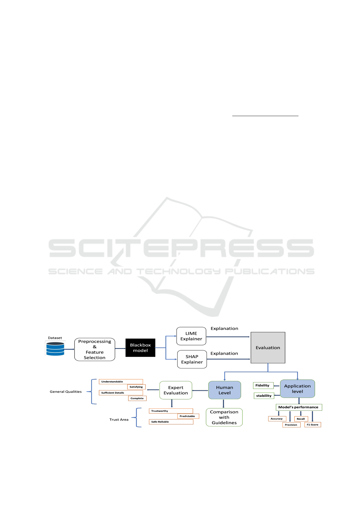
3 APPROACH
Figure 1 illustrate the layout of the experiment. Pre-
possessing steps involve handling missing values, re-
moving duplicates, and correcting errors, and feature
selection is carried out in consultation with the ex-
pert. A detail description of these steps is presented
in section-4. Randomforest is used as blackbox model
which is trained on the medical dataset for the pre-
diction of treatments for breast cancer patients. A
Random Forest is an ensemble learning method (Azar
et al., 2014). It works by constructing multiple de-
cision trees during training. Each tree in the forest
is built using a random subset of features and a ran-
dom subset of the training data, which helps ensure
that the trees are diverse and not excessively corre-
lated. This randomness improves classification ac-
curacy and gain better generalization ability (Parmar
et al., 2019). Our use case involves predicting five
treatment options, including surgery and four types
of therapies (Chemo, Target, Hormonal and Radio).
Figure 1: Evaluation of LIME and SHAP explainer through quantitative (Application-based) and qualitative (Human-based)
assessments.
HEALTHINF 2025 - 18th International Conference on Health Informatics
532

These therapies has further divided into four out-
puts/labels (pre − surgery, Post − surgery, pre and
post surgery and without surgery) which make this
problem multi-class multi-output problem. Two sur-
rogate models (LIME and SHAP ) are used to explain
the predictions of the blackbox model. LIME pro-
vides local approximation to explain individual pre-
dictions. On the other hand SHAP uses sharply values
from cooperative game theory to fairly distribute the
contribution of each feature to the prediction.
The explanations from both LIME and SHAP are
subjected to an extensive analysis. This process eval-
uates the effectiveness of each method in providing
meaningful insights into the model’s predictions. The
evaluation is taken place onto two levels: Human-
level and Application-level.
3.1 Application Level Evaluation
At application level, explanations are evaluated at fol-
lowing parameters:
3.1.1 Model’s Performance
In this section we will present the evaluation matrices
of black-box model. Accuracy measures the overall
correctness of the model and is calculated as the ra-
tio of correctly predicted instances to the total num-
ber of instances. Precision measures the accuracy
of the positive predictions made by the model. It
is calculated as the ratio of true-positive predictions
to the sum of true-positive and false-positive predic-
tions. Recall measures the model’s ability to identify
all relevant instances. It is calculated as the ratio of
true positive predictions to the sum of true positives
and false negatives. F1-score is the matrix which con-
siders both precision and recall. It is harmonic mean
of precision and recall, providing a balance between
the two metrics.
3.1.2 Fidelity
Although post-hoc explanation methods (Guidotti
et al., 2018) can be used to interpret black-box mod-
els, it is possible that the explanation generated is not
always faithful to the decision-making of the origi-
nal black box as the explanatory methods are differ-
ent from the prediction methods. Hence, it is im-
portant to understand how well explainable methods
can mimic the decision making process of black-box
models (Messalas et al., 2019). Fidelity measures the
similarity of prediction made by a black box and sur-
rogate model.
Consider an input feature vector x =
(x
1
, x
2
, . . . ,x
k
), prediction probability for predicted
class Y (x) and Z as set of pertubations z ∈ Z. Mean
absolute percentage error (MAPE), that computes the
difference in the prediction probabilities of surogate
model and black-box model, is used to measure the
fidelity of explanations (Velmurugan et al., 2021).
F =
∑
|Z|
1
|Y (z)−Y (z)|
Y (z)
|Z|
(10)
Fidelity can also be computed by using R-squared:
R
2
= 1 −
∑
k
i=1
( f (z
(i)
) − g(z
(i)
))
2
∑
k
i=1
( f (z
(i)
) −
¯
f )
2
(11)
Where f (z
(i)
) are predictions for perturbed samples
from the complex model, g(z(1)) are predictions for
perturbed samples from the surrogate model and
¯
f is
the mean of the original model’s predictions for the
perturbed samples:
¯
f =
1
k
k
∑
i=1
f (z
(i)
) (12)
A high R
2
value close to 1 indicates high fidelity,
meaning the surrogate model’s predictions closely
match those of the complex model.
3.1.3 Stability
The Stability Index (SI) compares the variables com-
position in the explanations E
1
, . . . ,E
m
, that are gen-
erated multiple times for the same instance.
We consider the set of all possible combinations (two
by two) C
2
m
(E
1
, . . . ,E
m
) of the m explanations for the
same instance. We define a measure of concordance
among the two explanations:
pair = (E
α
, E
β
) (13)
V
α
= {feat ∈ V : (E
α
(feat) ̸= 0} (14)
V
β
= {feat ∈ V : (E
β
(feat) ̸= 0} (15)
C
pair
= |V
α
∩V
β
| (16)
where V
α
and V
β
represent respectively the variables
used in the explanations E
α
and E
β
. The concor-
dance function C
pair
returns an integer value, namely
the cardinality of the intersection between V
α
and V
β
,
ranging from 0 to p, p is the number of variables
used by both V
α
and V
β
. For obtaining the VI in-
dex we evaluate the concordance over all the pairs in
C
2
m
(E
1
, . . . ,E
m
) and average them out.
V I =
∑
k
1
C
pair
p
|C
2
m
(E
1
, . . . ,E
m
)|
(17)
Can We Trust Explanation! Evaluation of Model-Agnostic Explanation Techniques on Highly Imbalanced, Multiclass-Multioutput
Classification Problem
533

3.2 Human Level Evaluation
In order to evaluate the quality of the explanation
generated using both LIME and SHAP, we compared
them with medical guidelines and also carried out a
human study.
3.2.1 Comparison with Guidelines
Medical guidelines are systematic statements that aid
practitioners in decision-making. They are based
on evidence and provide a framework for evaluating
patients, diagnosing conditions, and recommending
treatments.
Lets M is the complex machine learning model
and x is the instance for which explanations are gen-
erated. Explanation E
M
generated by model M can
be defined as:
E
LIME
(x) = {( f
i
, w
i
) : i = 1, 2, . . . , n} (18)
E
SHAP
(x) = {( f
i
, s
i
) : i = 1, 2, . . . , n} (19)
Where f
i
is the i-th feature, w
i
is its weight in the
LIME explanation and s
i
is SHAP value of i-th fea-
ture.
We define importance mapping function
Imp( f
i
, E) as:
Imp( f
i
, E) =
(
w
i
if E = E
LIME
s
i
if E = E
SHAP
(20)
We define the I
i
(G, E) as indicator function:
I
i
(G, E) = {( f
i
, Imp( f
i
, E), G
i
) : f
i
∈ G (21)
I
i
(G, E) =













if Imp( f
i
, E) > 0 and G
i
= High
1 or
Imp( f
i
, E) = 0 and G
i
= Low
0 Else
(22)
G is the set of medical guidelines, where G
i
∈ {High,
Medium, Low} represents the importance of feature
i. Comparison index Γ(G, E), that measures the con-
cordance scores between explanations and medical
guidelines, can be defined as:
Γ(E, G) =
1
|G|
|G|
∑
i=1
I
i
(23)
A high value of Γ(E , G) close to 1 indicates that the
explanations are completely matches the guidelines
and vice versa.
3.2.2 Expert Evaluation
After the detailed description of the considered ex-
planations, we focus now on the expert evaluation of
explanations. We conducted survey which consists of
two components: first, an introduction to the features
as we converted categorical features to numerical fea-
tures for training of black-box model. Second, we
presented explanations from LIME and SHAP to the
expert. We considered seven qualities: Understand,
Satisfying, Sufficient Details, Complete, Trustworthy,
Predictable and Safe-Reliable. The first four belong
to the class of general qualities, because they apply
universally to any explanation. While the later three
are the members of the trust area, which is crucial for
users to have confidence in the explanations. The clin-
ician can evaluate the quality of the explanations by
answering questions asked in the survey: giving an
integer evaluation between 1 (very bad) and 10 (very
good).
4 EXPERIMENT
This section first presents an overview of the dataset
used during experiments, followed by a detail descrip-
tion of the steps taken to prepare the dataset for this
study, including pre-processing, feature selection, and
handling class-imbalance.
4.1 Dataset
The Integraal Kankercentrum Nederland (IKNL) is
an organization dedicated to improving the quality of
cancer care in the Netherlands, and is established to
address the need for a coordinated and integrated ap-
proach to cancer prevention, treatment, and research.
The synthetic dataset (Integraal Kankercentrum Ned-
erland, 2021) retrieved from the IKNL comprises
breast cancer data of a total of 60 thousand patients
from 2010 to 2019. The data consists of 46 features,
including five target variables, named chemo therapy,
Table 1: Distribution of targets.
Modalities/Labels
Treatments
No-therapy Pre-surgical Post-surgical Pre- and post-surgical Without surgery
Chemotherapy 39145 7187 11909 734 1025
Hormonal therapy 26977 664 26828 1433 4098
Radio therapy 20277 1532 36875 - 1316
Targeted therapy 50889 1490 3183 2834 1604
Yes No
Surgery
5728 54272
HEALTHINF 2025 - 18th International Conference on Health Informatics
534

hormonal therapy, radiotherapy, targeted therapy and
surgery.
The data exploration revealed a total of 58,377
women and 1,623 men, with an average age of 62
years, ranging from 18 to 105 years old.
The distribution of the patients over the classes of
target variables can be seen in table 1.
4.2 Prepossessing
Features selection is carried out by incorporating
expert knowledge. After consulting with a physi-
cian, several features were deleted from the dataframe
which were irrelevant and have no influence on the
treatment prediction, such as the key ID of the pa-
tients and the tumor, the year o f incidence or the
localisation of the primary tumor (which is the same
for every patient).
Moreover, to handle missing values, each row
containing one or more missing values has been re-
moved. Due to the complex intrinsic relationships
between variables in the dataset, any fill-in method
would result in implausible combinations.
Additionally, one-hot encoding was applied to
convert categorical features into numerical form.
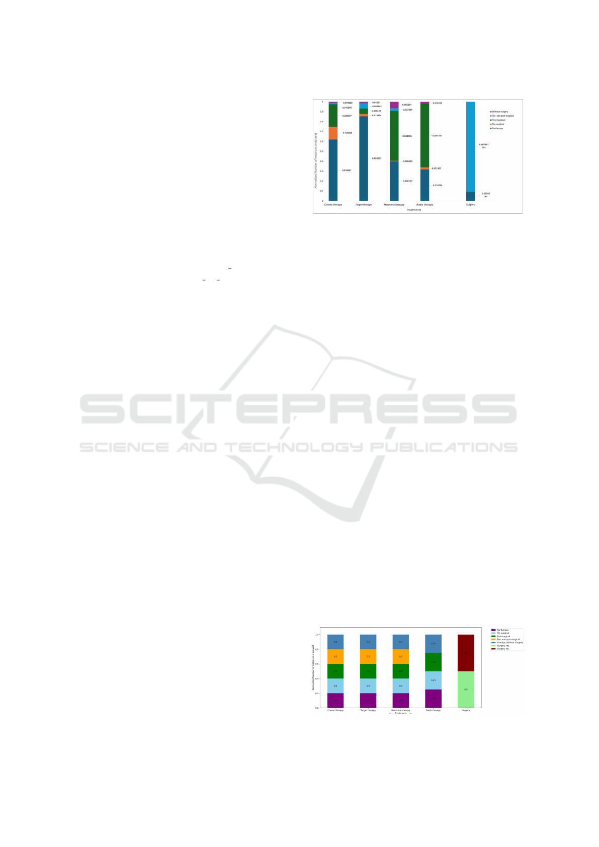
4.3 Class Imbalance Handling
Class imbalance between the target variables can be
seen in the figure 2. Five targets/classes are shown
along the x-axis. Each class has a number of out-
puts/labels that are represented in different colors.
For example, chemotherapy has five output / labels
(no therapy, pre-surgical, post-surgical, pre- and post-
surgical, and without surgery). Each segment within
the bars represents these labels by indicating the nor-
malized value from 0 to 1. To solve this problem
of class-imbalance, Synthetic Minority Oversampling
TEchnique (SMOTE) (Fern
´
andez et al., 2018) is uti-
lized. Where synthetic data is generated based on the
distance between a minority data point and its near-
est minority neighbor, thereby creating new synthetic
data points between the two minority data points. The
result is shown in the figure 3 where, for a particu-
lar Class, each segment within the bars has the same
normalized value. Thus, the new dataset has the same
number of instances for all the labels within the a spe-
cific class.
5 RESULT
The results presented in this section are obtained
by running the experiments on MacBook M3 using
Figure 2: Class imbalance for targeted treatments.
Python version 3.11.5. Our main goal is to evaluate
the explanations from the surrogate-models. We will
present results of application level and human level
evaluation in this section. SHAP and LIME provide a
way of explaining how individual features contribute
to the predictions of machine-learning models. The
explanation plot provides a clear and interpretable vi-
sualization of the most critical features influencing
the model’s prediction for specific treatment. Figure4
shows the explanation for predicting ”chemo-therapy
pre-surgery” treatment. The features here are ranked
according to their importance. The most important
feature is at the top, and vice-versa. In this figure, we
stated only the features that support the prediction of
”pre-surgical chemotherapy”. A complete participa-
tion of features presented in figure5, where the other
features are also included. Features in green colour
support the prediction and features in red colour op-
pose this prediction.
5.1 Results for Application Level
Evaluation
5.1.1 Model’s Performance
In this section, We evaluated the performance of black
box model. Dataset divided into train and test data
with a ratio of 80% and 20% respectively. We trained
the Randomforst classifier and evaluated it’s perfor-
mance using four primary metrics, accuracy, preci-
sion, recall and F1-score. Results are shown in the
table 2. It is evident that the classifier performs well
for all treatment’s prediction. Among them, the model
Figure 3: Balanced dataset after SMOTE.
Can We Trust Explanation! Evaluation of Model-Agnostic Explanation Techniques on Highly Imbalanced, Multiclass-Multioutput
Classification Problem
535

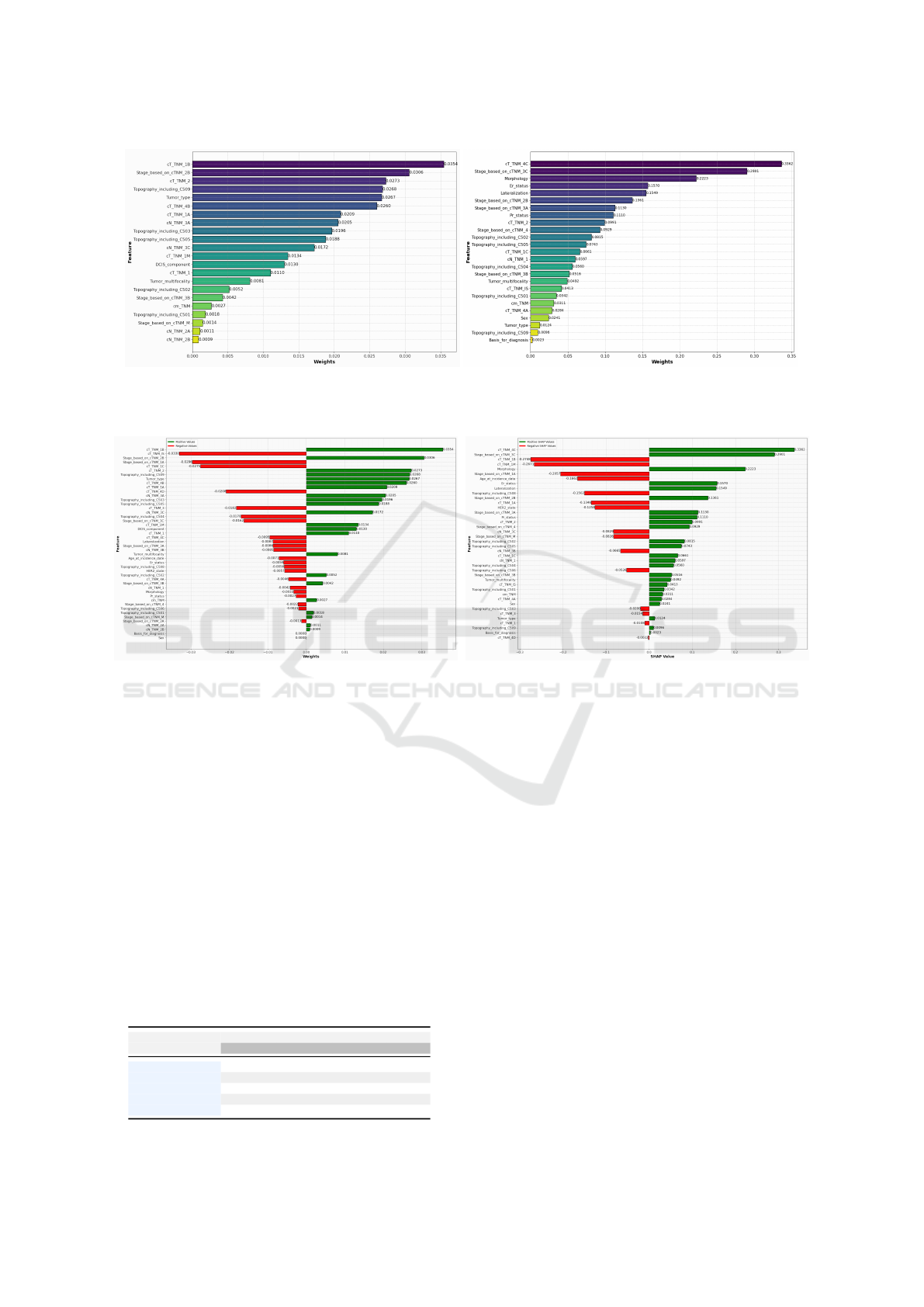
(a) Top features for single label prediction (by LIME) (b) Top features for single label prediction (by SHAP)
Figure 4: Top features, those supported the prediction of Pre-surgical Chemo Therapy, by both LIME and SHAP.
(a) Summery of LIME explanation for single label prediction (b) Summery of shap Explanation for single label prediction
Figure 5: Over all contribution of features (in-favour or opposite) for prediction of Pre-surgical Chemo Therapy provided by
both LIME and SHAP.
performed better for Hormonal-Therapy where we
obtained about 94% precision, F1 score, precision and
recall scores. On the other hand, we have the lowest
performance for Radio therapy which is about 76%
for all evaluation metrics. This performance demon-
strate that the model makes accurate prediction and
effectively identifies relevant cases.
5.1.2 Fidelity
Fidelity refers to how well the surrogate model ap-
proximates the predictions of the original complex
model for a given instance. It can have values be-
Table 2: Performance of black-box model for breast cancer
treatment prediction.
Performance Metrics
Treatments
Accuracy F1 scores Precision Recall
Chemotherapy 0.801 0.800 0.804 0.801
Hormonal therapy 0.947 0.947 0.948 0.947
Radio therapy 0.764 0.763 0.763 0.764
Targeted therapy 0.815 0.813 0.815 0.815
Surgery 0.934 0.934 0.936 0.934
tween 0 to 1. High fidelity indicates that the local sur-
rogate model’s predictions closely match those of the
complex model for the instance being explained. We
randomly selected 10 instances from the dataframe
and assessed the fidelity of LIME and SHAP across
5 classes. The boxplot in Figure 6 illustrates the fi-
delity scores of both LIME and SHAP. The graph
contains five pairs of box plots, each representing one
of the treatment modalities. A horizontal line inside
each box marks the median value. Overall, SHAP
has higher fidelity than LIME. The fidelity scores of
LIME for chemotherapy and radiotherapy were no-
tably low. For target therapy, the mean fidelity scores
of both LIME and SHAP were similar. Both explana-
tion methods showed better results for surgery treat-
ment prediction, which is a binary class.
5.1.3 Stability
To evaluate stability, we aimed to determine if the ex-
planations were consistent across the same instances
HEALTHINF 2025 - 18th International Conference on Health Informatics
536

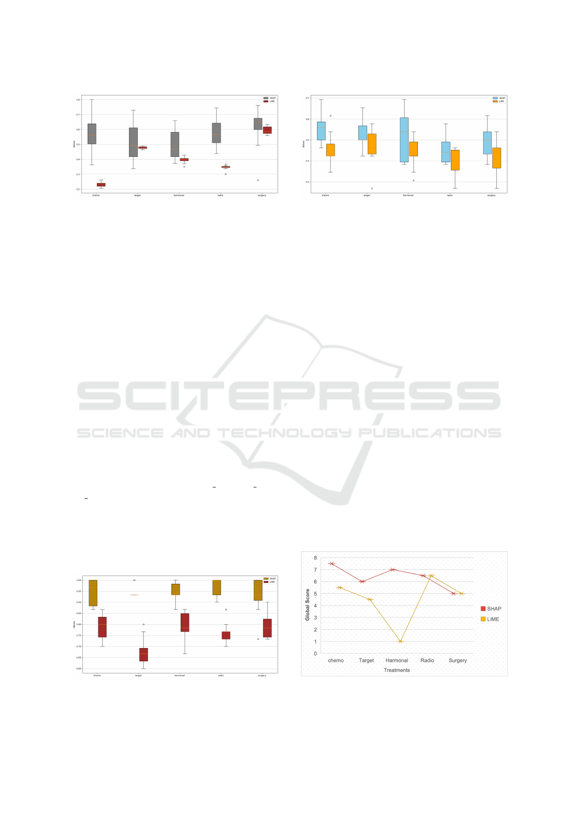
Figure 6: Fidelity score of LIME and SHAP over different
treatments modalities.
when generated multiple times. We randomly se-
lected 10 instances and, for each instance and each
target class, generated explanations 5 times under the
same model settings. We compared the feature com-
positions in these repeatedly generated explanations
for each instance and class. Figure 7 presents the
concordance of the top 5 features in the explanations
for each treatment. SHAP demonstrated better sta-
bility compared to LIME in this multi-class, multi-
output scenario. For some point, i.e. for target ther-
apy and hormonal therapy, LIME has lower median
and a slightly wider spread compared to SHAP.
5.2 Results for Human Level Evaluation
5.2.1 Comparison with Guideline
We have used the Oncoguide-2020 guidelines (Inte-
graal Kankercentrum Nederland, 2020) about breast
cancer developed by Integraal Kankercentrum Ned-
erland (IKNL). For our primary treatment predic-
tions, we extracted a portion of the relevant features
from these guidelines, such as [cT TNM, cN TNM,
cM TNM, Grade of tumor, Age, and HER2-status].
Figure 8 illustrate the concordance scores of two
explanation methods, SHAP and LIME, with med-
ical treatment guidelines across five different treat-
ment modalities: chemotherapy (’chemo’), targeted
therapy (’target’), hormonal therapy (’hormonal’), ra-
diotherapy (’radio’), and surgery (’surgery’). The
Figure 7: Stability score of LIME and SHAP for breast can-
cer treatment prediction.
Figure 8: Comparison of explanations with IKNL-
guideline.
concordance score measures how well the explana-
tions from each method align with established medi-
cal guidelines. A higher concordance score is better,
with an ideal value of 1.
The box-plot 8 shows that SHAP generally
achieves higher median concordance scores across all
treatment modalities compared to LIME. This sug-
gests that SHAP explanations are more consistently
aligned with medical guidelines. However, the vari-
ability within each method and modality indicates that
there are specific cases where the concordance can
vary significantly. This detailed visualization pro-
vides reliability and applicability of these explanation
methods in clinical settings.
5.3 Expert Evaluation
We generated explanation on randomly chosen sam-
ples from the dataset and asked expert/clinician to
judge the explanations and give score to these ex-
planation. On the basis of proposed qualities, ex-
pert can give score between 1( very bad) and 10
(vary good) to each explanation. The graph 9 il-
lustrate the aggregated average performance score of
two methods, LIME and SHAP, across multiple in-
stances. The graph highlights that SHAP is generally
preferred by experts over LIME for explaining predic-
tion tasks related to various breast cancer treatments.
Figure 9: Aggregated score from expert evaluation for dif-
ferent treatments.
Can We Trust Explanation! Evaluation of Model-Agnostic Explanation Techniques on Highly Imbalanced, Multiclass-Multioutput
Classification Problem
537

SHAP’s consistent performance makes it a more suit-
able choice for scenarios where explanation and reli-
ability is crucial.
This survey helps us to measure the credibility and
reliability of the explanation and also helps us to as-
sess the extent to which the explanation meets the ex-
pectations and needs of the experts.
6 CONCLUSIONS & FUTURE
WORK
In this paper we have presented a comprehensive and
detailed analysis of the explanation produced by post-
hoc explanations methods LIME and SHAP, for pre-
dicting breast cancer treatments using highly imbal-
anced IKNL systhetic dataset. We evaluated these
explanation on stability, fidelity, and their alignment
with established medical guidelines and expert evalu-
ations.
Our experiments showed that SHAP outperformed
LIME in terms of fidelity for this problem. This ad-
vantage is likely due to SHAP’s game theory foun-
dation and the use of Shapley values, which provide
a unique solution for feature importance allocation.
This robust nature of SHAP enhances the accuracy,
consistency, and reliability of explanations. On the
other hand, LIME offers local explanations by mod-
ifying the input data and fitting a simplified model
to approximate the original model’s behavior around
specific instances.
In terms of stability, which measures the consis-
tency of explanations across the same instances over
multiple runs, SHAP produced more stable explana-
tions compared to LIME for local predictions. How-
ever, SHAP can be more expensive considering com-
putations as there is a trade off between speed and
stability.
Comparing the human-level interpretation, SHAP
explanations were more consistently aligned with
medical guidelines and with the expert evaluation
than LIME. This could be attributed to LIME’s re-
liance on random sampling, which can introduce vari-
ability across different runs.
For robust and dependable explanations, particu-
larly in contexts demanding high fidelity, SHAP is a
more reliable option for interpreting machine learning
models.
In the healthcare industry, XAI is used very fre-
quently in clinical decision models to ensure trans-
parency and trustworthy analytics. It is applied to
manage clinical diagnosis (Zhang et al., 2022), drug
delivery (Jim
´
enez-Luna et al., 2020), disease classifi-
cation and treatment recommendations (Mellem et al.,
2021) (Shah et al., 2023) and other purposes.
LIME and SHAP are widely recognized as leading
model-agnostic XAI techniques. This study shows
that SHAP outperforms LIME in both qualitative and
quantitative assessments. However, these (LIME and
SHAP) are not the only model-agnostic XIA (Xu
et al., 2019) approaches available. Let us compare
them to other techniques by examining their limita-
tions and advantages:
- For simple models, partial dependency plots
(PDPs) and individual conditional expectation
plots (ICE) may be suitable. For complex mod-
els, LIME or SHAP might be more appropriate.
- If you need detailed explanations for individual
predictions, LIME is usually a good choice. For
global insights, SHAP, PDPs and sensitivity anal-
ysis are suitable.
- SHAP can be computationally expensive, espe-
cially for large datasets. LIME and PDPs are gen-
erally more efficient.
In our experiment, we utilized features listed in the
current IKNL medical guidelines, although the model
was trained on numerous other features. In future
studies:
- we can incorporate guidelines from additional
sources, including the American Cancer Society
(ACM) (Oeffinger et al., 2015) and National Insti-
tute for Health and Care Excellence (NICE) (Mur-
ray et al., 2009) to ensure clinical relevance and
accuracy.
- we can use other black-box ML models, i.e.
deep neural network (DNN) (Samek et al., 2016),
extreme learning machines (ELM) (Shah et al.,
2019) and deep reinforcement learning (DRL)
(Arulkumaran et al., 2017) to assess their impact
on the outcomes, generalizability, and robustness.
- we can also compare LIME and SHAP explana-
tions with those from interpretable models such
as Explainable Boosting Machine (EBM) (Chen
et al., 2021) and Bayesian Networks (BN) (Scana-
gatta et al., 2019).
ACKNOWLEDGEMENTS
This work has been partly supported by the PersOn
project (P21-03), which has received funding from
Nederlandse Organisatie voor Wetenschappelijk On-
derzoek (NWO).
HEALTHINF 2025 - 18th International Conference on Health Informatics
538

REFERENCES
Arulkumaran, K., Deisenroth, M. P., Brundage, M., and
Bharath, A. A. (2017). Deep reinforcement learning:
A brief survey. IEEE Signal Processing Magazine,
34(6):26–38.
Azar, A. T., Elshazly, H. I., Hassanien, A. E., and Elko-
rany, A. M. (2014). A random forest classifier for
lymph diseases. Computer methods and programs in
biomedicine, 113(2):465–473.
Chen, Z., Tan, S., Nori, H., Inkpen, K., Lou, Y., and
Caruana, R. (2021). Using explainable boosting ma-
chines (ebms) to detect common flaws in data. In
Joint European Conference on Machine Learning and
Knowledge Discovery in Databases, pages 534–551.
Springer.
Fern
´
andez, A., Garcia, S., Herrera, F., and Chawla, N. V.
(2018). Smote for learning from imbalanced data:
progress and challenges, marking the 15-year an-
niversary. Journal of artificial intelligence research,
61:863–905.
Garreau, D. and Luxburg, U. (2020). Explaining the ex-
plainer: A first theoretical analysis of lime. In Interna-
tional conference on artificial intelligence and statis-
tics, pages 1287–1296. PMLR.
Guidotti, R., Monreale, A., Ruggieri, S., Turini, F., Gian-
notti, F., and Pedreschi, D. (2018). A survey of meth-
ods for explaining black box models. ACM computing
surveys (CSUR), 51(5):1–42.
Integraal Kankercentrum Nederland (2020). Integraal
kankercentrum nederland (iknl). Accessed: 2024-07-
26.
Integraal Kankercentrum Nederland (2021). Synthetic
dataset. Accessed: 2024-07-26.
Jim
´
enez-Luna, J., Grisoni, F., and Schneider, G. (2020).
Drug discovery with explainable artificial intelligence.
Nature Machine Intelligence, 2(10):573–584.
Kumar, I. E., Venkatasubramanian, S., Scheidegger, C., and
Friedler, S. (2020). Problems with shapley-value-
based explanations as feature importance measures.
Lundberg, S. M. and Lee, S.-I. (2017). A unified approach
to interpreting model predictions. Advances in neural
information processing systems, 30.
Mellem, M. S., Kollada, M., Tiller, J., and Lauritzen, T.
(2021). Explainable ai enables clinical trial patient se-
lection to retrospectively improve treatment effects in
schizophrenia. BMC medical informatics and decision
making, 21(1):162.
Meng, Y., Yang, N., Qian, Z., and Zhang, G. (2020). What
makes an online review more helpful: an interpreta-
tion framework using xgboost and shap values. Jour-
nal of Theoretical and Applied Electronic Commerce
Research, 16(3):466–490.
Messalas, A., Kanellopoulos, Y., and Makris, C. (2019).
Model-agnostic interpretability with shapley values.
In 2019 10th International Conference on Informa-
tion, Intelligence, Systems and Applications (IISA),
pages 1–7. IEEE.
Murray, N., Winstanley, J., Bennett, A., and Francis, K.
(2009). Diagnosis and treatment of advanced breast
cancer: summary of nice guidance. Bmj, 338.
Oeffinger, K. C., Fontham, E. T., Etzioni, R., Herzig,
A., Michaelson, J. S., Shih, Y.-C. T., Walter, L. C.,
Church, T. R., Flowers, C. R., LaMonte, S. J., et al.
(2015). Breast cancer screening for women at average
risk: 2015 guideline update from the american cancer
society. Jama, 314(15):1599–1614.
Parmar, A., Katariya, R., and Patel, V. (2019). A review
on random forest: An ensemble classifier. In Inter-
national conference on intelligent data communica-
tion technologies and internet of things (ICICI) 2018,
pages 758–763. Springer.
Ribeiro, M. T., Singh, S., and Guestrin, C. (2016). ”why
should i trust you?”: Explaining the predictions of any
classifier.
Samek, W., Binder, A., Montavon, G., Lapuschkin, S., and
M
¨
uller, K.-R. (2016). Evaluating the visualization
of what a deep neural network has learned. IEEE
transactions on neural networks and learning systems,
28(11):2660–2673.
Scanagatta, M., Salmer
´
on, A., and Stella, F. (2019). A sur-
vey on bayesian network structure learning from data.
Progress in Artificial Intelligence, 8(4):425–439.
Shah, S. I. H., Alam, S., Ghauri, S. A., Hussain, A., and
Ansari, F. A. (2019). A novel hybrid cuckoo search-
extreme learning machine approach for modulation
classification. IEEE Access, 7:90525–90537.
Shah, S. I. H., De Pietro, G., Paragliola, G., and Coro-
nato, A. (2023). Projection based inverse reinforce-
ment learning for the analysis of dynamic treatment
regimes. Applied Intelligence, 53(11):14072–14084.
ˇ
Strumbelj, E. and Kononenko, I. (2014). Explaining pre-
diction models and individual predictions with feature
contributions. Knowledge and information systems,
41:647–665.
Velmurugan, M., Ouyang, C., Moreira, C., and Sindhgatta,
R. (2021). Evaluating fidelity of explainable methods
for predictive process analytics. In International con-
ference on advanced information systems engineer-
ing, pages 64–72. Springer.
Xu, F., Uszkoreit, H., Du, Y., Fan, W., Zhao, D., and Zhu,
J. (2019). Explainable ai: A brief survey on his-
tory, research areas, approaches and challenges. In
Natural language processing and Chinese computing:
8th cCF international conference, NLPCC 2019, dun-
huang, China, October 9–14, 2019, proceedings, part
II 8, pages 563–574. Springer.
Zhang, Y., Weng, Y., and Lund, J. (2022). Applications
of explainable artificial intelligence in diagnosis and
surgery. Diagnostics, 12(2):237.
Can We Trust Explanation! Evaluation of Model-Agnostic Explanation Techniques on Highly Imbalanced, Multiclass-Multioutput
Classification Problem
539