A Mixed Quantization Approach for Data-Free Quantization of LLMs

Feng Zhang

1 a

, Yanbin Liu

1,∗ b

, Weihua Li

1 c

, Xiaodan Wang

2,∗ d

and Quan Bai

3 e

Auckland University of Technology, Auckland, New Zealand

Yanbian University, Jilin, China

University of Tasmania, Hobart, Australia

yxr1097@autuni.ac.nz, {yanbin.liu, weihua.li}@aut.ac.nz,

Keywords:

Quantization, Large Language Model, Linear Programming, Transformer, PTQ, LLama-2.

Abstract:

Large Language Models (LLMs) have demonstrated signiﬁcant capabilities in intelligent activities such as

natural language comprehension, content generation, and knowledge retrieval. However, training and deploy-

ing these models require substantial computation resources, setting up a signiﬁcant barrier for developing AI

applications and conducting research. Various model compression techniques have been developed to address

the demanding computational resource issue. Nonetheless, there has been limited exploration into high-level

quantization strategy to offer better ﬂexibility of balancing the trade-off between memory usage and accu-

racy. We propose an effective mixed-quantization method named MXQ to bridge this research gap for a better

memory-accuracy balance. Speciﬁcally, we observe that the weight distributions of LLMs vary considerably

from layer to layer, resulting in different tolerances to quantization errors. Motivated by this, we derive a

novel quantization optimisation formulation to solve for the layer-wise quantization parameters, while enforc-

ing the overall quantization memory consumption budget into the constraints. The new formulation can be

efﬁciently solved by converting to a mixed integer programming problem. Experiments shows that our method

can achieve the 1% accuracy loss goal with additional bit budget or further reduce memory usage on Llama

models. This unlocks a wide range of quantization options and simpliﬁes memory-accuracy trade-off.

1 INTRODUCTION

When deploying or ﬁne-tuning pre-trained Large Lan-

guage Models (LLMs), GPUs are typically employed

to accelerate the neural network’s forward and back-

ward propagation processes. These specialized pro-

cessors excel at executing massive parallel opera-

tions, such as large-scale matrix multiplication (Baji,

2018). To minimize latency, the model parameters,

gradients, and associated optimizer states are stored

in GPU memory using high-precision numeric rep-

resentations like ﬂoat16 or ﬂoat32. However, this

approach often proves inadequate in addressing the

increasing computational resource demands resulting

from the exponential growth in parameters of pre-

trained LLMs, driven by the scaling laws (Kaplan

https://orcid.org/0009-0007-1891-6403

https://orcid.org/0000-0003-4724-8065

https://orcid.org/0000-0001-9215-4979

https://orcid.org/0009-0008-2159-2339

https://orcid.org/0000-0003-1214-6317

∗

Corresponding author

et al., 2020). The high computational demands have

hindered research on large LLMs (Ding et al., 2023),

as only very limited researches surveyed were able to

conduct practical experiments due to the prohibitive

costs of deploying large pre-trained language models

to validate their hypotheses experimentally.

Fortunately, an innovative model compression

technique, known as model quantization, has been de-

veloped to tackle this challenge and signiﬁcantly re-

duce storage requirements. Quantization is a tech-

nique used to convert the high-precision numeric

representation of large pre-trained models’ parame-

ters into compact, low-bit equivalents. This process

reduces memory consumption and boosts inference

speed. Although current quantization methods strive

to preserve model precision as much as possible,

some loss of accuracy is inevitable. It is almost im-

possible for a quantized model to maintain the exact

accuracy of the unquantized model. The quantization

research community typically aims for near-lossless

compression, commonly considered to be within 1%

error relative to the uncompressed baseline, as deﬁned

Zhang, F., Liu, Y., Li, W., Wang, X. and Bai, Q.

A Mixed Quantization Approach for Data-Free Quantization of LLMs.

DOI: 10.5220/0013159100003890

Paper published under CC license (CC BY-NC-ND 4.0)

In Proceedings of the 17th International Conference on Agents and Artiﬁcial Intelligence (ICAART 2025) - Volume 2, pages 353-363

ISBN: 978-989-758-737-5; ISSN: 2184-433X

353

Quantization Grid

Gaussian

K-means

RTN

Calibration Dataset

Original Model

Optimization

Quantized Weights

and Meta Data

Quantized Model

*.pth

*.safetensors

Figure 1: Model quantization converts an original model to the quantized model with several steps: quantization grid, optimi-

sation with calibration dataset, and quantized weights and metadata storage.

in the MLCommons benchmark (Reddi et al., 2020).

The key challenge of quantization lies in the trade-off

between reducing the memory requirements and pre-

serving the model performance.

The general pipeline of a model quantization pro-

cess is shown in Figure 1. First, the quantization

method maps the original high-precision numeric rep-

resentation of parameters into a narrower range of val-

ues, known as quantization grids or bins, allowing

them to be packed into fewer bits. Then, an optimisa-

tion step is usually employed to compensate for quan-

tization errors, which may require additional metrics,

such as a calibration dataset. After that, adjacent

weights are packed into the same byte to save space.

The associated metadata are usually quantized using

the same process to further reduce storage, which is

also known as double-quantization in (Dettmers et al.,

2023). Finally, the quantized model is saved in persis-

tent storage for distribution.

However, existing methods using this approach

lack ﬂexible controls of the memory-accuracy balance

since they tend to adopt identical quantization conﬁg-

urations across all weight matrices with diverse dis-

tributions. To tackle this issue, we propose a novel

mixed-quantization method named MXQ, which can

offer a broader spectrum of options for memory-

accuracy trade-off and simplify memory management

by using intuitive bit budget.

Speciﬁcally, we conducted a comprehensive in-

vestigation on the weight distribution of all neural net-

work layers in Llama family models and observed an

intriguing phenomenon: the MLP and self-attention

modules exhibit signiﬁcantly distinct weight distribu-

tions across various layers, as shown in Figure 2. For

example, mlp.down proj has a wider weight band

while mlp.gate proj owns a much narrower one.

In addition, the Kurtosis line plots indicate the start-

ing and ending layers tend to exhibit higher Kurto-

sis value, which demonstrates the degree of quantiza-

tion difﬁculty varies signiﬁcantly across different lay-

ers. Motivated by this observation, we design a new

quantization optimisation formulation by introducing

a set of layer-wise conﬁgurations to handle their dis-

tinctive distributions. Moreover, the memory budget

is controlled by a well-devised storage cost function

in the formulation constraints. For efﬁcient optimi-

sation, we convert the quantization formulation to a

mixed integer linear programming (MiLP) problem.

The quantization error matrices and storage cost ma-

trices are pre-computed before solving the LP prob-

lem to accelerate the overall quantization process.

Comprehensive experiments were conducted to

validate the effectiveness of MXQ on language mod-

els, showing a good balance between memory storage

and model performance. The contributions of this pa-

per are summarized as follows:

• We propose an effective quantization method

named MXQ for precise budget control and ﬂex-

ible memory-accuracy balance. MXQ provides

a novel optimisation formulation with layer-wise

conﬁgurations in the objective and a storage cost

function in the constraints.

• The new formulation is transformed into a mixed

integer linear programming (MiLP) problem,

which can be solved with efﬁcient off-the-shell LP

solvers, which contributes to fast quantization.

• Experiments are performed on perplexity bench-

marks for the Llama family of language mod-

els, showing ﬂexible control and better memory-

accuracy balance over state-of-the-art quantiza-

tion methods.

ICAART 2025 - 17th International Conference on Agents and Artiﬁcial Intelligence

354

100

150

200

kurtosis

0.00

0.25

0.50

0.75

1.00

1.25

0 10 20 30 40

input_layernorm(2.048e+05)

Absolute Value

5.0

7.5

10.0

12.5

kurtosis

0.0

0.5

1.0

1.5

2.0

2.5

0 10 20 30 40

mlp.down_proj(2.831e+09)

Absolute Value

kurtosis

0.0

0.2

0.4

0.6

0.8

0 10 20 30 40

mlp.gate_proj(2.831e+09)

Absolute Value

3.0

3.3

3.6

3.9

4.2

kurtosis

0.0

0.5

1.0

1.5

0 10 20 30 40

mlp.up_proj(2.831e+09)

Absolute Value

500

1000

1500

2000

2500

kurtosis

0.0

0.5

1.0

1.5

0 10 20 30 40

post_attention_layernorm(2.048e+05)

Absolute Value

kurtosis

0.0

0.2

0.4

0.6

0.8

0 10 20 30 40

self_attn.k_proj(1.049e+09)

Absolute Value

kurtosis

0.00

0.25

0.50

0.75

1.00

1.25

0 10 20 30 40

self_attn.o_proj(1.049e+09)

Absolute Value

100

kurtosis

0.00

0.25

0.50

0.75

1.00

0 10 20 30 40

self_attn.q_proj(1.049e+09)

Absolute Value

nth percentile 100 99.99 99.9 99 0

kurtosis

0.0

0.2

0.4

0 10 20 30 40

self_attn.v_proj(1.049e+09)

Absolute Value

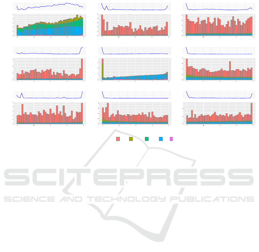
Figure 2: This ﬁgure illustrates the weight distributions across all layers of the Llama-2-13B model, represented by various

percentiles (0%, 99%, 99.9%, 99.99%, and 100%). The numbers in parentheses the total parameters of each module. The

Kurtosis line plot shows the degree of deviation from a normal distribution, where a value of 3 indicates no deviation. The

higher Kurtosis value denotes greater divergence thus greater difﬁculty to quantize accurately. The varying column heights and

the Kurtosis line plot highlight distinct patterns across different layers, motivating the design of a novel layer-wise quantization

method. This ﬁgure is best viewed in color and with zoom for clarity.

2 RELATED WORKS

The Quantization techniques have been extensively

explored, and numerous innovative methods were in-

vented and applied in a variety of use cases, such

as inference (Frantar et al., 2023; Lin et al., 2023),

ﬁne-tuning (Dettmers et al., 2023; Guo et al., 2024)

and optimizer state (Dettmers et al., 2022). These

techniques can be generally categorised into two

categories: (1) Quantization Aware Training (QAT)

(Nagel et al., 2021), requiring backward propagation

and being tightly coupled with model training, and

(2) Post Training Quantization (PTQ) (Nagel et al.,

2019), which is a training-free methodology. PTQ

has been recognised as the mainstream due to the

substantial number of pre-trained LLMs. For ex-

ample, the HuggingFace model search page reports

around 700,000 models published as of June 2024.

Consequently, advancements in PTQ research provide

greater practical values.

In this paper, we focus on a speciﬁc class of the

PTQ method, i.e., weight-only quantization method.

Speciﬁcally, considering whether an extra calibration

dataset is adopted during quantization, weight-only

method can be further divided into two categories:

calibration-based methods and calibration-free meth-

ods. Below, we survey the papers most relevant to our

proposed mixed-quantization method.

2.1 Calibration-Based Methods

The calibration-based approaches, based on advanced

mathematical theory such as the Hessian matrix and

Fisher information, usually produce better-quantized

models. However, they tend to be slow and prone to

overﬁtting the calibration dataset. The representative

state-of-the-art implementations of calibration-based

approaches include GPTQ and AWQ.

GPTQ (Frantar et al., 2023) is based on Optimal

Brain Quantizer (OBQ) (Frantar and Alistarh, 2022),

which quantized one weight at a time while con-

stantly updating all not-yet-quantized weights to

compensate for the error incurred by quantizing a

single weight. GPTQ improves OBQ by quantizing

weight column-wise to eliminate repeated calculation

of the inverse of the Hessian Matrix, thus scaling

to a larger model with parameters as many as a few

hundred billion. GPTQ has extensively optimized

kernels to accelerate mixed-precision matrix multi-

A Mixed Quantization Approach for Data-Free Quantization of LLMs

355

plication. Thus, the GPTQ quantized models not only

save memory but also run faster.

AWQ (Lin et al., 2023), based the observation that the

importance of LLM’s weights is non-uniform, pro-

poses a quantization method to identify the minor-

ity “salient” weights by measuring activation magni-

tude and scaling the identiﬁed weights to minimize

quantization errors. What makes AWQ unique is that

rather than isolating salient weights into separate stor-

age like sparse matrix, it utilises the same quantized

storage to preserve the salient weights, eliminating

the need to develop specialised mixed-precision ma-

trix multiplication kernel for fast inference.

2.2 Calibration-Free Methods

HQQ (Badri and Shaji, 2023) approaches minimiz-

ing quantization errors by relying solely on the weight

without considering the layer activation. Further-

more, it incorporates the L

p<1

-norm loss function to

effectively model outliers through a hyper-Laplacian

distribution, which captures the long-tailed nature of

outlier errors more accurately than the squared error,

resulting in a better representation of error distribu-

tion. The outstanding feature of HQQ lies in its ex-

traordinary quantization speed, which achieves a very

close performance compared to the top quantization

methods.

BnB (Dettmers et al., 2023) employs a novel high-

precision technique to quantize pre-trained model

weights to 4-bit NormalFloat(NF4), which employs

the Gaussian distribution exhibited in model weights.

The 4-bit NormalFloat datatype represents 16 val-

ues (q1,q2,·· · , q16) in the interval [−1,1]. Each

weight matrix is chunked into small groups for bet-

ter quantization accuracy. Additionally, NF4 employs

the double quantization technique to reduce the over-

head introduced by granular group-wise quantization,

a widely adopted strategy by other state-of–the-art

quantization methods.

3 MIXED QUANTIZATION

METHOD

Previous studies on quantizing LLMs (Dettmers et al.,

2023; Frantar et al., 2023; Lin et al., 2023; Badri

and Shaji, 2023) employed identical quantization con-

ﬁgurations across entire model. This approach lacks

ﬂexibility in balancing the trade-off between memory

consumption and model performance under various

resource constraints and may be sub-optimal, espe-

cially in billion-scale LLMs as demonstrated in ﬁg-

Table 1: The mixed quantization conﬁgurations.

Parameter Values

2,3,4,8

32,64,128

128

ure 2, where some layers exhibit far taller weight

bands and spikes in Kurtosis line, indicating not all

layers are equally quantizable. This necessitates a

new approach that employs non-uniform quantization

settings for optimal quantization.

MXQ allocates optimal quantization conﬁgura-

tions to each weight matrix according to a user-

speciﬁed overall bit budget for each parameter to

minimize the global quantization error. Speciﬁcally,

MXQ identiﬁes ideal conﬁgurations that minimize

the sum of Frobenius norm of the difference between

the original matrices and their quantized counterparts

while conﬁning the memory usage within the con-

straint of the target memory budget. Thus the problem

can be formulated as a Mixed integer Linear Program-

ming (Huangfu and Hall, 2018) problem. Let’s denote

= (b

) as the conﬁguration parameters

used to quantize the ith matrix of the LLM, where b

and g

denote the bit width and group size for quan-

tizing weights, b

and g

indicate the bit width and

group size to quantize metadata, such as zero points

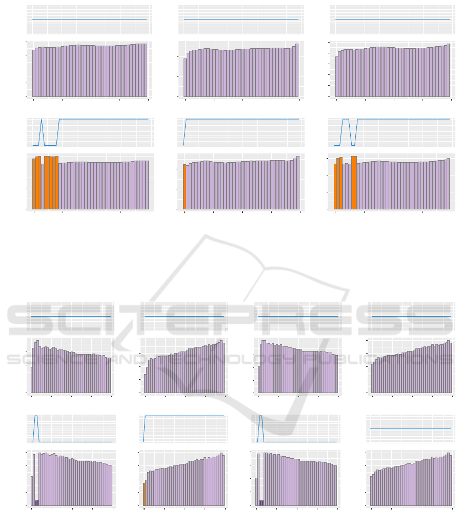
and scales. For a visual explanation of the bit width

and group size, refer to Figure 8 in the appendix.

Let C be the set of all possible conﬁgurations. In

this paper, we limit the search space as listed in Table

1, leading to the cardinality of all possible conﬁgura-

tions to be 12. Moreover, let {W

(i)

}

i=1

be the set of N

matrices in the LLM to be quantized. The MXQ qua-

tization probelm can be formulated as an optimisation

problem with equation 1.

argmin

,···,c

∑

i∈{1,...N}

∈C



(i)

−

(i)



s.t.

∑

i∈{1,...N}

∈C

storage(W

(i)

) ≤ β,

(1)

where parameter β denotes the overall memory bud-

get for the quantized model in megabytes. The stor-

age cost function stor is deﬁned in Equation 2:

stor(W

(i)

) = |W

(i)

| ·



· g



(2)

For simplicity, we use the same second-level bit width

and group size for scales and zeroes, as variations

in these conﬁgurations have minor impact on overall

memory consumption.

ICAART 2025 - 17th International Conference on Agents and Artiﬁcial Intelligence

356

To minimize the objective function in Equation 1,

we calculate Frobenius norms and storage costs with

respect to all possible conﬁgurations (N × |C| in to-

tal) for a given LLM. To accelerate the process, the

Frobenius norm and storage cost can be pre-computed

and stored in two matrices beforehand, denoted as

F ∈ R

N×|C|

and S ∈ R

N×|C|

. With these pre-computed

metrics in place, the optimal quantization conﬁgu-

rations problem is re-formulated as a mixed integer

linear programming problem by introducing a series

of binary decision variables x

, where j ∈ {1,. ..,M}

and M = N × |C|. Speciﬁcally, the optimisation prob-

lem can be formulated as follows:

argmin

F · X

s.t. S · X ≤ β,

A · X =













N×1

(3)

where X =













M×1

∈ {0, 1} ∀ j ∈ {1, . ..,M},

F =



··· f



S =



··· s



A =







|C|

z }| {

1,··· ,1

|C|

z }| {

0,··· ,0 · · ·

|C|

z }| {

0,··· ,0

|C|

z }| {

0,··· ,0

|C|

z }| {

1,··· ,1 · · ·

|C|

z }| {

0,··· ,0

|C|

z }| {

0,··· ,0

|C|

z }| {

0,··· ,0 · · ·

|C|

z }| {

1,··· ,1







N×M

As we search for one optimal conﬁguration out

of |C| for a total number of N matrices, we initial-

ize A ∈ R

N×M

in Equation 3, i.e., a matrix of N rows

by M columns with only 0’s and 1’s. Each row con-

tains |C| consecutive ones corresponding to positions

of the weight matrices encoded in A. Equation 3

can be solved efﬁciently by off-the-shelf LP solvers

such as Gurobi (Gurobi Optimization, LLC, 2023)

and HiGHS (Huangfu and Hall, 2018). In this pa-

per, the scipy wrapper of HiGHS is adopted to solve

Equation 3.

4 EXPERIMENTS

Theoretically, our method can be extended to support

quantization methods that support layer-wise conﬁg-

urations. However, limited by time and computation

resources, we focused our experiments on leveraging

HQQ (Badri and Shaji, 2023) as the underlying quan-

tization implementation due to its impressive quanti-

zation speed and outstanding accuracy. The design

of the experiments primarily emphasizes the 3- and

4-bit quantization as these conﬁgurations better pre-

serve the performance of LLMs (Dettmers and Zettle-

moyer, 2023). Besides the perplexity, which is a strin-

gent measurement of accuracy and generally reﬂects

true performance of the LLM (Dettmers and Zettle-

moyer, 2023). Additionally, we benchmarked quanti-

zation speed and actual GPU memory consumption in

order to evaluate the quantization algorithms compre-

hensively.

We evaluated the performance of our MXQ on the

state-of-art large language models such as the Llama

family models to verify the efﬁcacy of the MXQ. The

selected baselines were simultaneously tested under

the same experimental settings. To facilitate the ex-

periment and maximize reproducibility, we developed

a harness tool named lm-quant-toolkit, open-sourced

on GitHub, to execute the experiments and collect

data. The procedures to execute the experiments are

elaborated in the appendix 5.

4.1 Settings

The proposed method was applied to the Llama (Tou-

vron et al., 2023) family models, including Llama-2-

7B, Llama-2-13B, and Llama-3-8B. We employed the

Hugging Face(huggingface, 2024) perplexity evalu-

ation method, which is slightly different from those

used in prior works and tends to yield lower values

than those reported in existing research, on the two

datasets: WikiText-2 (Merity et al., 2016) and C4

(Raffel et al., 2020) respectively. The current state-of-

the-art calibration-based and calibration-free quanti-

zation methods are adopted as the baselines, including

HQQ (Badri and Shaji, 2023), BnB (Dettmers et al.,

2023), GPTQ (Frantar et al., 2023) and AWQ (Lin

et al., 2023). These baselines were re-evaluated with

3 or 4-bit conﬁgurations according to Table 1, ensur-

ing a fair comparison.

All the experiments were conducted on a Linux

workstation with Nvidia RTX 4090 GPU. The hard-

ware and software speciﬁcations are presented in the

Table 3. The Llama models, published by Meta, were

fetched from the HuggingFace.

A Mixed Quantization Approach for Data-Free Quantization of LLMs

357

Table 2: This table presents the perplexity metrics of the proposed MXQ method along with various baseline methods on the

Llama family models. The table includes some of MXQ’s representative bit budgets, ranging from 3.07 to 6.89. As the budget

increases, the MXQ’s perplexity approaches or even surpasses the state-of-the-art methods, demonstrating its effectiveness in

prioritizing accuracy over memory.

Llama-2-7B Llama-2-13B Llama-3-8B

Method Conﬁg BPP

↓WikiText2

↓C4

↓MEM

↓WikiText2 ↓C4 ↓MEM ↓WikiText2 ↓C4 ↓MEM

FP16 - 16 5.18 6.95 12.55 4.63 6.45 19.21 5.81 8.98 14.96

HQQ

g32

4.51 5.28 7.06 4.07 4.69 6.51 7.63 6.07 9.41 5.82

MXQ 4.51 5.29 7.08 3.89 4.69 6.51 7.28 6.11 9.47 5.62

GPTQ

4.51 5.39 7.11 4.74 4.72 6.54 8.43 8.80 10.44 6.71

AWQ 4.51 5.26 7.04 3.98 4.69 6.51 7.59 6.07 9.39 5.72

HQQ

g64

4.25 5.30 7.11 3.79 4.70 6.54 7.07 6.19 9.60 5.51

MXQ 4.25 5.31 7.13 3.71 4.71 6.54 6.90 6.29 9.76 5.49

GPTQ 4.25 5.39 7.13 4.50 4.73 6.56 7.97 11.83 11.77 6.46

AWQ 4.25 5.29 7.07 3.74 4.71 6.53 7.10 6.15 9.52 5.46

HQQ

g128

4.13 5.35 7.16 3.65 4.74 6.57 6.80 6.38 9.94 5.36

MXQ 4.13 5.33 7.17 3.72 4.74 6.57 6.94 6.40 9.96 5.54

BnB

4.13 5.32 7.12 3.60 4.72 6.55 6.71 6.20 9.64 5.31

GPTQ 4.13 5.39 7.18 4.39 4.74 6.57 7.74 97.03 27.77 6.33

AWQ 4.13 5.31 7.10 3.62 4.71 6.55 6.92 6.21 9.67 5.33

HQQ

g32

3.51 5.62 7.53 4.07 4.89 6.78 7.63 7.09 11.16 5.82

MXQ 3.51 5.65 7.63 4.17 4.92 6.84 7.54 7.30 11.68 6.16

GPTQ 3.51 5.94 7.81 3.20 5.09 6.96 5.93 17.76 17.98 4.88

AWQ

3.51 - - - - - - - - -

HQQ

g64

3.25 5.82 7.80 3.41 4.98 6.94 6.33 7.80 12.35 5.11

MXQ 3.25 6.04 8.13 3.98 5.06 7.05 7.18 9.52 15.23 5.80

GPTQ 3.25 6.13 8.07 2.98 5.14 7.06 5.49 11.16 14.33 4.64

AWQ 3.25 - - - - - - - - -

HQQ

g128

3.13 6.20 8.39 3.08 5.15 7.14 5.69 9.31 14.90 4.75

MXQ 3.13 6.36 8.60 3.85 5.24 7.34 6.92 12.23 19.49 5.67

GPTQ 3.13 6.32 8.30 2.87 5.24 7.19 5.27 52.78 30.04 4.52

AWQ 3.13 - - - - - - - - -

MXQ

6.89 6.89 5.25 7.01 6.40 4.66 6.48 11.91 6.01 9.30 8.49

5.72 5.72 5.26 7.03 5.54 4.67 6.50 10.22 6.04 9.35 7.57

5.02 5.02 5.28 7.05 5.01 4.68 6.50 9.18 6.05 9.38 7.00

4.21 4.21 5.32 7.14 4.43 4.72 6.55 8.04 6.34 9.84 6.46

4.17 4.17 5.33 7.16 4.44 4.73 6.56 8.07 6.38 9.93 6.48

4.11 4.11 5.34 7.18 4.46 4.74 6.58 8.10 6.42 9.99 6.50

4.07 4.07 5.36 7.21 4.44 4.75 6.59 8.12 6.46 10.08 6.53

3.95 3.95 5.43 7.29 4.44 4.79 6.65 8.06 6.59 10.36 6.45

3.87 3.87 5.45 7.33 4.46 4.81 6.67 8.12 6.73 10.59 6.35

3.83 3.83 5.46 7.36 4.42 4.82 6.69 8.04 6.80 10.71 6.30

3.65 3.65 5.54 7.50 4.32 4.87 6.76 7.81 7.09 11.24 6.27

3.19 3.19 6.15 8.30 3.91 5.11 7.12 7.05 11.20 17.89 5.73

3.15 3.15 6.25 8.45 3.87 5.18 7.25 6.96 12.02 19.10 5.69

3.11 3.11 6.49 8.75 3.82 5.30 7.43 6.88 12.52 20.16 5.65

3.07 3.07 6.78 9.12 3.78 5.57 7.72 6.80 13.54 21.40 5.61

Bit per parameter, i.e. the average bits a paratemer takes.

Perplexity on the WikiText2 dataset, evaluation follows the HuggingFace algorithm (huggingface, 2024).

Perplexity on a subset of the C4 dataset, which is composed of the ﬁrst 1,100 entries of the en validation split.

Memory is measured using PyTorch’s API after loading the quantized model into GPU. This column is reported in GiB.

We used github.com/AutoGPTQ/AutoGPTQ for this experiment.

The 4-bit BnB employes 64 as the group size. However, the bit per parameter is 4.13 according to (Dettmers et al., 2023).

The github.com/casper-hansen/AutoAWQ used by this experiment has no 3-bit quantization implementation.

Additional bit budgets unavailable to other baseline methods.

ICAART 2025 - 17th International Conference on Agents and Artiﬁcial Intelligence

358

FP16

Llama−2−13B

65707580

2.8 3.0 3.2 3.4 3.6 3.8 4.0 4.2 4.4 4.6 4.8 5.0 5.2 5.4

4.63

4.83

5.03

5.23

5.43

FP16

Llama−2−13B

−1012

% Degradation

Method: MXQ FP16 BnB HQQ

% Memory Reduction

Bit Budget

Perplexity

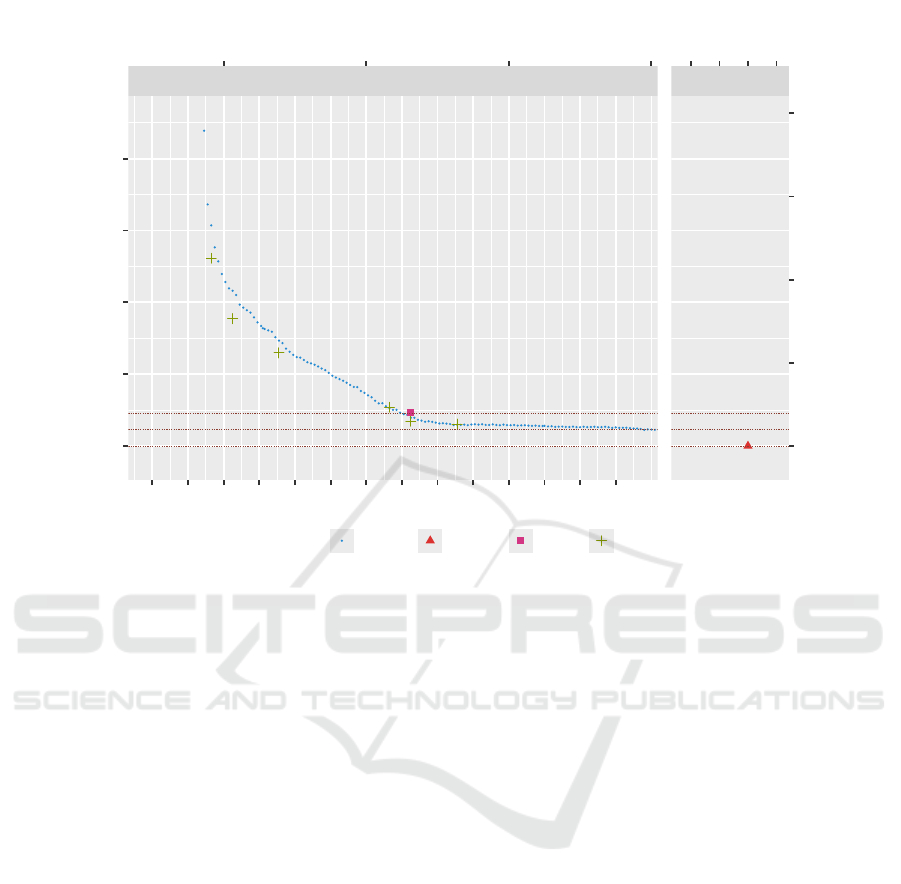
Figure 3: This ﬁgure illustrates the potential trade-offs between memory and perplexity within the 3-bit to 5-bit range for the

Llama-2-13B models on the WikiText2 dataset using the calibration-free quantization methods such as HQQ and BnB. The

red triangle at the lower right corner denotes the FP16 baseline. The gaps between the there horizontal lines represent the 1%

and 2% perplexity degradation ranges respectively. The tiny square indicates the BnB performance. As evidenced by this plot,

MXQ offers far more options to balance memory and performance. It achieves the 1% performance loss goal at a bit budget

around 5.6. Additionally, it enables aggressive 77% memory saving at a bit budget around 3.7 while maintaining perplexity

drop within 5%.

4.2 Results and Analysis

The perplexity metrics for various Llama models are

presented in Table 2. The evaluation results for our

mixed quantization method are shown as the “MXQ”

rows at the bottom of the table. We tested a few hun-

dred bit budgets, ranging from 2.75 to 7.75, some of

the representative bit budgets as listed in the Table 2.

The upper section of the table displays the results for

HQQ, GPTQ, and AWQ under various bit and group

size settings. The ﬁrst column denotes the quantiza-

tion method, while second column indicates the com-

bination of bit width and group size.

Figure 3 presents the broader range of quantiza-

tion options and the corresponding performance met-

rics within the 3-bit to 5-bit range for the Llama-2-

13B models on the WikiText2 dataset on the Llama-

2-13B model. The calibration-free quantization meth-

ods such as HQQ and BnB are included as reference.

The red triangle at the lower right corner denotes the

FP16 baseline. The gaps between the there horizontal

lines represent the 1% and 2% perplexity drop zones.

MXQ offers a ﬂexible trade-off between memory

consumption and accuracy by unlocking a variety of

budget-perplexity options, showing good potential for

real application with diverse memory constraints. On

one hand, MXQ can leverage slightly larger memory

budget for better accuracy, which is not an option for

the existing methods. As demonstrated in Table 2, at

the bit budget of 6.89, MXQ surpasses all SoTA meth-

ods on WikiText2 and C4 perplexity metrcis for all the

three Llama models. Additionally, MXQ achieves the

1% performance loss goal at a bit budget around 5.6

on the Llama-2-13B model as evidenced in the Fig-

ure 3. On the other hand, MXQ enables aggressive

memory reduction. As illustrated by Figure 3, MXQ

achieves approximately 77% memory saving at a bit

budget around 3.7 while maintaining perplexity drop

within 5% on the Llama-2-13B model.

In addition to evaluating perplexity, we conducted

a comprehensive assessment of the actual GPU mem-

ory consumption and quantization time of MXQ and

A Mixed Quantization Approach for Data-Free Quantization of LLMs

359

HQQ

GPTQ

AWQ

FP16

MXQ

HQQ

GPTQ

AWQ

FP16

MXQ

HQQ

GPTQ

AWQ

FP16

MXQ

HQQ

GPTQ

AWQ

FP16

MXQ

HQQ

GPTQ

AWQ

FP16

MXQ

HQQ

GPTQ

AWQ

FP16

MXQ

HQQ

GPTQ

AWQ

FP16

MXQ

HQQ

GPTQ

AWQ

FP16

MXQ

HQQ

GPTQ

AWQ

FP16

MXQ

Llama−2−7B

Llama−3−8B

Llama−2−13B

b4g32

b4g64

b4g128

0 4 8 12 16 20 0 4 8 12 16 20 0 4 8 12 16 20

Figure 4: This ﬁgure illustrates the GPU memory usage,

measured in gigabytes(GiB) when loading baseline and

quantized Llama models into GPU prior to executing any

inference. All quantized models exhibit a substantial reduc-

tion in memory consumption when compared to the FP16

baseline. Notably, the MXQ approach offers additional

memory saving comparing to HQQ.

the baseline quantization methods on the Llama mod-

els. As presented in Figure 4, all quantization meth-

ods demonstrate signiﬁcant drop in memory usage,

decreasing it to approximately one-third of the mem-

ory required by the unquantized models. Notably,

MXQ exhibits additional memory reduction when

compared to HQQ. With respect to the quantization

time, despite the fact that MXQ incurs small overhead

on the MiLP algorithm to ﬁnd optimal quantization

conﬁgurations, it is able to quantize the Llama-2 13B

model within 1 mintue, which is an order of magni-

tude smaller than the AWQ and GPTQ.

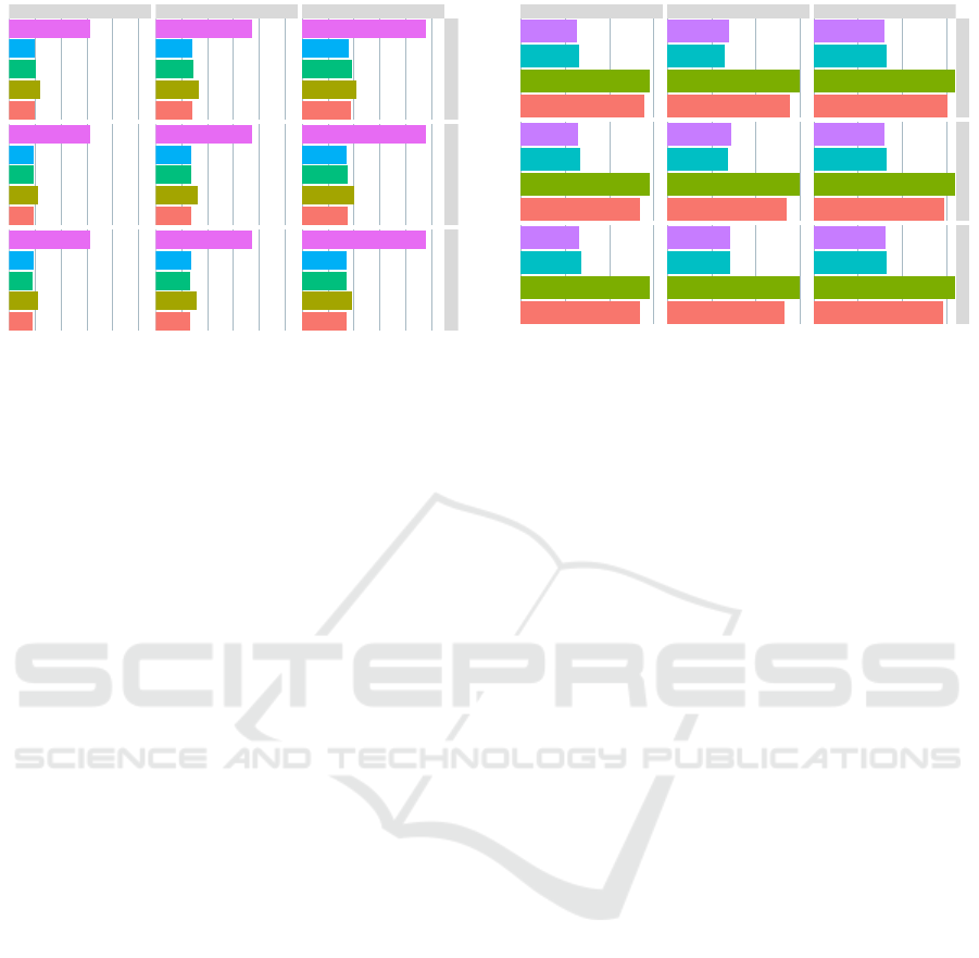
Lastly, we examined the differences between

MXQ and HQQ in bit budget allocation. The Fig-

ure 6 and 7 present the quantization conﬁg assigments

for the MLP and self attention modules of Llama-2-

13B model respectively. As demonstrated by the ﬁg-

ures, HQQ allocates identical bit bugdets to all lay-

ers and modules. In contrast, MXQ tends to sacri-

ﬁce the initial layers of the MLP modules to favor the

second and third layer of the self attention modules,

speciﬁcally the K and Q. This approach aligns with

the MiLP formulation deﬁned in Equation 3, which

aims to minimize the sum of Frobenius norms and sat-

isfy the memory constraints. We veriﬁed the sum of

Frobenius norms produced by MXQ is indeed smaller

than the that of HQQ.

5 CONCLUSION

The mixed quantization (MXQ) represents an ef-

fective approach to optimizing the balance between

GPTQ

HQQ

AWQ

MXQ

GPTQ

HQQ

AWQ

MXQ

GPTQ

HQQ

AWQ

MXQ

GPTQ

HQQ

AWQ

MXQ

GPTQ

HQQ

AWQ

MXQ

GPTQ

HQQ

AWQ

MXQ

AWQ

GPTQ

HQQ

MXQ

AWQ

GPTQ

HQQ

MXQ

AWQ

GPTQ

HQQ

MXQ

Llama−2−7B

Llama−3−8B

Llama−2−13B

b4g32

b4g64

b4g128

100

1000

100

1000

100

1000

Figure 5: This ﬁgure compares the quantization time of

various quantization methods: MXQ, HQQ, AWQ, GPTQ.

The three Llama variants: Llama-2-7B, Llama-2-13B and

Llama-3-8B, are evaluated using b4g32, b4g64 and b4g128

conﬁgurations on a NIVDIA RTX 4090 GPU. The quan-

tization time is measured in seconds and displayed in log

scale (log10). Notably, GPTQ and AWQ quantization are

approximately an order of magnitude slower than MXQ and

HQQ.

model accuracy and memory consumption. By speci-

fying a bit budget, this methodology offers a broader

spectrum of quantization options, enabling the identi-

ﬁcation of optimal quantization conﬁgurations to en-

hance existing quantization methods. This innovative

optimization formulation to allow us to solve layer-

wise quantization parameters, incorporating memory

budget constraints. This approach enables our method

to offer an advantageous memory-performance bal-

ance when quantizing transformer-based large mod-

els. Incorporating the proposed MXQ into the repos-

itory of quantization utilities would constitute a valu-

able supplement, enriching the tools available for op-

timizing increasingly larger transformer-based mod-

els.

Future work will focus on enhancing the accuracy

of MXQ and extending its generalizability by experi-

menting with other transformer-based language mod-

els and multi-modal models. Furthermore, we plan

to incorporate end-to-end benchmarks such as IFEval,

BBH, MATH Level 5, GPQA, MUSR, and MMLU-

PRO in our evaluations to ensure the robustness of the

proposed method’s performance on real-world tasks.

ICAART 2025 - 17th International Conference on Agents and Artiﬁcial Intelligence

360

38.00

38.02

38.04

38.06

38.08

Memory(MiB)

b4g32

0 10 20 30 40

HQQ − mlp.down_proj

FNorm

38.00

38.02

38.04

38.06

38.08

Memory(MiB)

b4g32

0 10 20 30 40

HQQ − mlp.gate_proj

FNorm

38.00

38.02

38.04

38.06

38.08

Memory(MiB)

b4g32

0.0

2.5

5.0

7.5

10.0

12.5

0 10 20 30 40

HQQ − mlp.up_proj

FNorm

36.0

36.5

37.0

37.5

38.0

Memory(MiB)

b4g64

b4g32

b4g64

b4g32

0 10 20 30 40

MXQ − mlp.down_proj

FNorm

36.0

36.5

37.0

37.5

38.0

Memory(MiB)

b4g64

b4g32

0 10 20 30 40

MXQ − mlp.gate_proj

FNorm

36.0

36.5

37.0

37.5

38.0

Memory(MiB)

b4g64

b4g32

b4g64

b4g32

0 10 20 30 40

MXQ − mlp.up_proj

FNorm

Figure 6: This ﬁgure presents a comparison of quantization conﬁguration allocations for the MLP modules in the Llama-

2-13B model, as determined by MXQ and HQQ, under a bit budget of 4.51. The column diagrams depict the assigned

quantization conﬁgurations, with light purple columns indicating the b4g32 conﬁguration, while the accompanying line plots

show memory usage in megabytes. Taller columns correspond to greater quantization errors. Notably, MXQ tends to sacriﬁce

the budgets of MLP modules in the initial layers. This ﬁgure should be viewed in color and zoomed in for optimal clarity.

14.04

14.06

14.08

14.10

14.12

Memory(MiB)

b4g32

0 10 20 30 40

HQQ − self_attn.k_proj

FNorm

14.04

14.06

14.08

14.10

14.12

Memory(MiB)

b4g32

0 10 20 30 40

HQQ − self_attn.o_proj

FNorm

14.04

14.06

14.08

14.10

14.12

Memory(MiB)

b4g32

0.0

2.5

5.0

7.5

10.0

0 10 20 30 40

HQQ − self_attn.q_proj

FNorm

14.04

14.06

14.08

14.10

14.12

Memory(MiB)

b4g32

0 10 20 30 40

HQQ − self_attn.v_proj

FNorm

Memory(MiB)

b8g128

b4g32

0.0

2.5

5.0

7.5

10.0

0 10 20 30 40

MXQ − self_attn.k_proj

FNorm

13.3

13.5

13.7

13.9

14.1

Memory(MiB)

b4g64

b4g32

0 10 20 30 40

MXQ − self_attn.o_proj

FNorm

Memory(MiB)

b8g128

b4g32

0.0

2.5

5.0

7.5

10.0

0 10 20 30 40

MXQ − self_attn.q_proj

FNorm

14.04

14.06

14.08

14.10

14.12

Memory(MiB)

b4g32

0 10 20 30 40

MXQ − self_attn.v_proj

FNorm

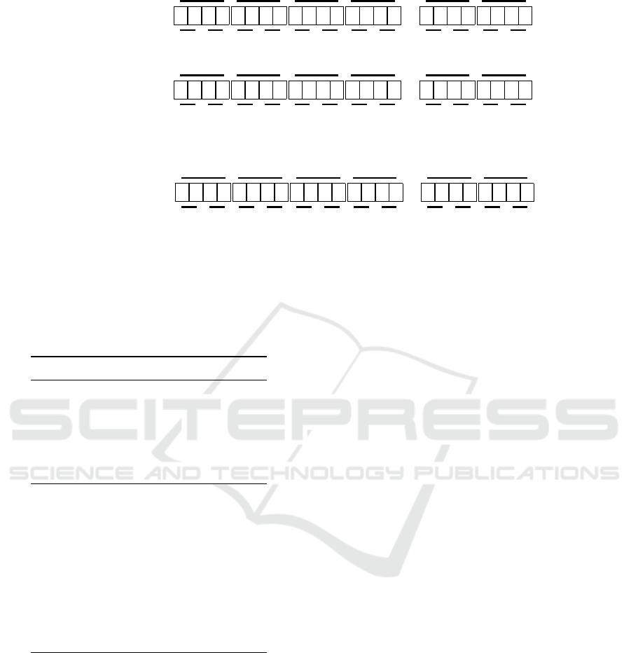
Figure 7: This ﬁgure presents a comparison of quantization conﬁguration allocations for the self attention modules in the

Llama-2-13B model under a bit budget of 4.51. The column diagrams depict the assigned quantization conﬁgurations, with

light purple columns indicating the b4g32 conﬁguration, while the accompanying line plots show memory usage in megabytes.

Taller columns correspond to greater quantization errors. As demonstrated in this ﬁgure, MXQ assigns bit bugdets aggres-

sively to the second and third layer of self attention modules (K and Q) to mininize sum of FNorm. This ﬁgure is best viewed

in color and with zoom for clarity.

A Mixed Quantization Approach for Data-Free Quantization of LLMs

361

REFERENCES

Badri, H. and Shaji, A. (2023). Half-quadratic quantization

of large machine learning models.

Baji, T. (2018). Evolution of the GPU Device widely used

in AI and Massive Parallel Processing. In 2018 IEEE

2nd Electron Devices Technology and Manufacturing

Conference (EDTM), pages 7–9.

Dettmers, T., Lewis, M., Shleifer, S., and Zettlemoyer, L.

(2022). 8-bit Optimizers via Block-wise Quantization.

arXiv:2110.02861 [cs].

Dettmers, T., Pagnoni, A., Holtzman, A., and Zettlemoyer,

L. (2023). QLoRA: Efﬁcient Finetuning of Quantized

LLMs. arXiv:2305.14314 [cs].

Dettmers, T. and Zettlemoyer, L. (2023). The case for 4-bit

precision: k-bit Inference Scaling Laws. In Proceed-

ings of the 40th International Conference on Machine

Learning, pages 7750–7774. PMLR. ISSN: 2640-

3498.

Ding, N., Qin, Y., Yang, G., Wei, F., Yang, Z., Su,

Y., Hu, S., Chen, Y., Chan, C.-M., Chen, W., Yi,

J., Zhao, W., Wang, X., Liu, Z., Zheng, H.-T.,

Chen, J., Liu, Y., Tang, J., Li, J., and Sun, M.

(2023). Parameter-efﬁcient ﬁne-tuning of large-scale

pre-trained language models. Nature Machine Intel-

ligence, 5(3):220–235. Publisher: Nature Publishing

Group.

Frantar, E. and Alistarh, D. (2022). Optimal brain compres-

sion: A framework for accurate post-training quanti-

zation and pruning. Advances in Neural Information

Processing Systems, 35:4475–4488.

Frantar, E., Ashkboos, S., Hoeﬂer, T., and Alistarh,

D. (2023). GPTQ: Accurate Post-Training Quan-

tization for Generative Pre-trained Transformers.

arXiv:2210.17323 [cs].

Guo, H., Greengard, P., Xing, E. P., and Kim, Y. (2024).

LQ-LoRA: Low-rank Plus Quantized Matrix Decom-

position for Efﬁcient Language Model Finetuning.

arXiv:2311.12023 [cs].

Gurobi Optimization, LLC (2023). Gurobi Optimizer Ref-

erence Manual.

Huangfu, Q. and Hall, J. A. J. (2018). Parallelizing the dual

revised simplex method. Mathematical Programming

Computation, 10(1):119–142.

huggingface (2024). Perplexity of ﬁxed-length models.

Kaplan, J., McCandlish, S., Henighan, T., Brown, T. B.,

Chess, B., Child, R., Gray, S., Radford, A., Wu, J.,

and Amodei, D. (2020). Scaling Laws for Neural Lan-

guage Models. arXiv:2001.08361 [cs, stat].

Lin, J., Tang, J., Tang, H., Yang, S., Dang, X., and Han,

S. (2023). AWQ: Activation-aware Weight Quantiza-

tion for LLM Compression and Acceleration. arXiv

preprint arXiv:2306.00978.

Merity, S., Xiong, C., Bradbury, J., and Socher, R. (2016).

Pointer Sentinel Mixture Models. arXiv:1609.07843

[cs].

Nagel, M., Baalen, M. v., Blankevoort, T., and Welling,

M. (2019). Data-Free Quantization Through Weight

Equalization and Bias Correction. pages 1325–1334.

Nagel, M., Fournarakis, M., Amjad, R. A., Bondarenko,

Y., van Baalen, M., and Blankevoort, T. (2021).

A White Paper on Neural Network Quantization.

arXiv:2106.08295 [cs].

Raffel, C., Shazeer, N., Roberts, A., Lee, K., Narang, S.,

Matena, M., Zhou, Y., Li, W., and Liu, P. J. (2020).

Exploring the Limits of Transfer Learning with a Uni-

ﬁed Text-to-Text Transformer. Journal of Machine

Learning Research, 21(140):1–67.

Reddi, V. J., Cheng, C., Kanter, D., and Mattson, P. a. e.

(2020). MLPerf Inference Benchmark. In 2020

ACM/IEEE 47th Annual International Symposium on

Computer Architecture (ISCA), pages 446–459.

Touvron, H., Martin, L., and Stone, K. e. a. (2023). Llama

2: Open Foundation and Fine-Tuned Chat Models.

arXiv:2307.09288 [cs].

APPENDIX

Experiments Procedure

The results presented in the previous sections were

produced by conducting experiments on the Llama

family models. The Llama model experiments in-

clude quantization and perplexity evaluation.

The specialized harness tool named lm-quant-

toolkit facilitates the tasks to quantize, evaluate lan-

guage and vision transformer models using the pro-

posed MXQ method as well as the baselines such as

HQQ, AWQ, GPTQ. This harness is designed to per-

form long-running experiments. It tracks the experi-

ment status and automatically resumes interrupted ex-

periment from last failed point. It collects experiment

duration, GPU memory consumption and key met-

rics such as perplexity and Open LLM LeaderBoard

scores. It consolidates outputs from sub-tasks into

experiment dataset in .csv format for further analysis

and reporting.

The quantization and evaluation of LLMs re-

quire substantial computation and storage resources.

Our experiment environment’s hardware and software

conﬁgurations are presented in Table 3.

The patched softwares need to be cloned from

github, as noted under Table 3, then be installed using

the PIP’s editable install method as they haven’t been

integrated in the upstream yet. Additional Python

libraries are automatically installed when the lm-

quant-toolkit is installed. For complete dependen-

cies, please review the ‘pyproject.toml‘ ﬁle of the lm-

quant-toolkit project.

The three Llama models, published on Hug-

ging Face by Meta, employed in this experiment

are the Llama-2-7B(meta-llama/Llama-2-7b-hf),

Llama-2-13B(meta-llama/Llama-2-13b-hf) and

ICAART 2025 - 17th International Conference on Agents and Artiﬁcial Intelligence

362

Group 1

1byte

z }| {

| {z }

1byte

z }| {

| {z }

···

1byte

z }| {

| {z }

Group 2

1byte

z }| {

| {z }

1byte

z }| {

| {z }

···

1byte

z }| {

| {z }

127

| {z }

128

Group m

1byte

z }| {

| {z }

n−63

| {z }

n−62

1byte

z }| {

| {z }

n−61

| {z }

n−60

···

1byte

z }| {

| {z }

n−1

| {z }

Figure 8: This ﬁgure illustrates the mapping of parameters in large language models (LLMs) to a low-bit representation with

a bit width of 4 and a group size of 64 (denoted as b

= 4,g

= 64 or simply b4g64). The small square boxes represent the bits

used to store the quantized parameters. In this scheme, a total of n parameters are divided into m = n/64 groups, with each

quantized parameter occupying 4 bits. To optimize memory storage, two successive parameters are packed into a single byte.

Additionally, per-group metadata, such as scales and zero points, are quantized using a similar approach but with a distinct bit

width and group size, referred to as b

and g

, respectively.

Table 3: Experiment hardware/software conﬁguration

Item Conﬁguation

CPU Intel i9-14900KF

Memory 192 GiB

Disk HP SSD FX900 Pro

2TB x 2

GPU NVIDIA GeForce

RTX 4090

OS Ubuntu 24.04

Python 3.11.9

CUDA 12.5

PyTorch 2.4.1

lm-quant-toolkit master

AutoAWQ 0.2.5

AutoGPTQ ea829c7 with the

CUDA 12.5 patch

HQQ aad6868 with MXQ

patch

The lm-quant-toolkit is published on github:

https://github.com/schnell18/lm-quant-toolkit.

The CUDA 12.5 patch can be fetched from:

https://github.com/schnell18/AutoGPTQ.

The MXQ patch can be fetched from:

https://github.com/schnell18/hqq.

Llama-3-8B(meta-llama/Meta-Llama-3-8B). The

main procedure to reproduce the language model

experiment results consists of:

1. evaluate the FP16 baseline’s perplexity metrics

on WikiText2 and C4 dataset for original Llama

models

2. quantize the selected Llama models using AWQ,

GPTQ, HQQ with conﬁgurations b4g32, b4g64,

b4g128, b3g32, b3g64 and b3g128

3. evaluate perplexity metrics on WikiText2 and C4

dataset for the AWQ, GPTQ and HQQ quantized

models

4. quantize the selected Llama models using MXQ

with a wide range of bit budgets ranging from 3.07

to 8.51

5. evaluate perplexity metrics on WikiText2 and C4

dataset for the MXQ quantized models

6. aggregate, analyze and visualize experiment re-

sults using R

The lm-quant-toolkit includes bash scripts to au-

tomate the aforementioned evaluation tasks. The re-

sults of the evaluation tasks, formatted as .csv ﬁles,

are stored in the experiment directories speciﬁed in

the corresponding task script. The quantized models

are stored under the snapshot directory speciﬁed in

the quantization scripts.

For future reference, the experiment result .csv

ﬁles are archived under the data-vis/data folder in

the lm-quant-toolkit repository with the compan-

ion R scripts to visualize the experiment data located

under the data-vis folder.

A Mixed Quantization Approach for Data-Free Quantization of LLMs

363