Distribution Controlled Clustering of Time Series Segments by Reduced

Embeddings

abor Sz

ucs

, Marcell Bal

azs T

oth

and Marcell N

emeth

Budapest University of Technology and Economics, Department of Telecommunications and Artiﬁcial Intelligence, Hungary

Keywords:

Clustering, Time Series Segments, Kolmogorov–Smirnov Test, COP-KMeans, Clustering Evaluation,

Conﬁdence Score.

Abstract:

This paper introduces a novel framework for clustering time series segments, addressing challenges like tem-

poral misalignment, varying segment lengths, and computational inefﬁciencies. The method combines the

Kolmogorov–Smirnov (KS) test for statistical segment comparison and adapted COP-KMeans for clustering

with temporal constraints. To enhance scalability, we propose a basepoint selection strategy for embedding

the time series segments that reduces the computational complexity from O(n

) to O(n · b) by limiting com-

parisons to representative basepoints. The approach is evaluated on diverse time series datasets from domains

such as motion tracking and medical signals. Results show improved runtime performance over traditional

methods, particularly for large datasets. In addition, we introduce a conﬁdence score to quantify the reliability

of cluster assignments, with higher accuracy achieved by ﬁltering low-conﬁdence segments. We evaluated

clustering performance using the Rand Index (RI), Adjusted Rand Index (ARI), and Normalized Mutual Infor-

mation (NMI). Our results demonstrate advantageous properties of the method in handling noise and different

time series data, making it suitable for large scale applications.

1 INTRODUCTION

Time series clustering is a crucial task in machine

learning with applications across various domains,

including ﬁnance, healthcare, and industry. It in-

volves grouping similar sequences of data points that

evolve over time. However, this process poses chal-

lenges due to temporal dependencies and varying seg-

ment lengths. Traditional methods, such as whole

time series and subsequence clustering (Aghabozorgi

et al., 2015; Zolhavarieh et al., 2014; Caiado et al.,

2015; Fujimaki et al., 2008), either struggle with large

datasets or fail to account for such complexities.

Subsequence clustering, which partitions a long

time series into segments for clustering, is particularly

relevant for identifying recurring patterns in datasets.

However, existing approaches often have difﬁculty in

dealing with temporal misalignment and variability in

segment length. Furthermore, at large datasets, the

computational inefﬁciency of traditional clustering al-

gorithms is a signiﬁcant limitation.

https://orcid.org/0000-0002-5781-1088

https://orcid.org/0009-0007-7136-314X

https://orcid.org/0009-0002-2835-0363

In this paper, we propose a novel clustering frame-

work that integrates the Kolmogorov-Smirnov (KS)

test (Kolmogorov, 1933) for statistical comparison

of segments to address temporal misalignment. To

further enhance clustering, we apply COP-KMeans

(Wagstaff et al., 2001), incorporating pairwise con-

straints to ensure that consecutive time series seg-

ments are not assigned to the same cluster, thereby

preserving their temporal independence. Our method

effectively handles large datasets while maintaining

accuracy. The key contributions of this paper are:

• A new subsequence clustering method combining

KS test statistic and adapted constrained cluster-

ing algorithm (COP-KMeans) for ﬂexible time se-

ries segment clustering.

• A reduced-embedding-based clustering method

with base point selection to decrease computa-

tional complexity.

• Comprehensive experimental results demonstrat-

ing the method’s efﬁciency and accuracy on di-

verse datasets.

• A conﬁdence score to quantify the reliability

of cluster assignments, where higher accuracy

achieved by ﬁltering low-conﬁdence segments.

SzÅ

scs, G., Tóth, M. B. and Németh, M.

Distribution Controlled Clustering of Time Series Segments by Reduced Embeddings.

DOI: 10.5220/0013162700003905

Paper published under CC license (CC BY-NC-ND 4.0)

In Proceedings of the 14th International Conference on Pattern Recognition Applications and Methods (ICPRAM 2025), pages 43-54

ISBN: 978-989-758-730-6; ISSN: 2184-4313

The remainder of this paper is organized as fol-

lows: Section 2 reviews related work, Section 3 ex-

plains the theoretical foundations, Section 4 and Sec-

tion 5 detail the proposed approach, and Section 6

presents experimental results and in the Section 7 we

draw the conclusions.

2 RELATED WORKS

The literature on time series clustering can be clas-

siﬁed into three main categories: whole time series,

subsequence, and time-point clustering (Aghabozorgi

et al., 2015; Zolhavarieh et al., 2014).

Whole time series clustering involves clustering a

set of individual time series (where each time series

is treated as a distinct instance for the clustering algo-

rithm) based on their similarity. This category has the

most extensive body of research and can be further di-

vided into three subcategories: shape-based, feature-

based, and model-based approaches.

In the shape-based approach (Meesrikamolkul

et al., 2012; Li et al., 2022), the shapes of two time

series are aligned as closely as possible by apply-

ing non-linear stretching and contracting along the

time axes. In the feature-based approach (Hautamaki

et al., 2008), raw time series data are transformed into

lower-dimensional feature vectors, which are then

used as inputs for traditional clustering algorithms.

Finally, in model-based methods (Liao, 2005), the

raw time series are converted into model parameters,

and clustering is performed based on these extracted

parameters using an appropriate distance measure.

Subsequence clustering (Keogh and Lin, 2005;

Zolhavarieh et al., 2014) focuses on clustering subse-

quences extracted from a single long time series, typi-

cally through a sliding window or other segmentation

techniques. The goal is to cluster these segments, and

this is the primary focus of our paper.

Time-point clustering (M

orchen et al., 2005; Ertl

et al., 2021), the third category, involves clustering

individual time points based on their temporal prox-

imity and the similarity of their corresponding values.

This method is similar to time series segmentation but

allows for some points to remain unclustered, treating

them as noise.

Several methods have been proposed for subse-

quence clustering. For example, the MDL framework

(Rakthanmanon et al., 2012) is a highly efﬁcient ap-

proach for time series clustering and can be applied

to data streams. Building on this foundational work,

Li et al. (Li et al., 2012) developed a methodology

to discover approximate time series motifs of varying

lengths using a compression algorithm.

Some researchers have proposed selective cluster-

ing of subsequences, emphasizing that subsequence

clustering is more meaningful when noisy or irrel-

evant subsequences are ignored and when subse-

quences of varying lengths are considered (Rodpong-

pun et al., 2012). Another approach by Yang (Yang

and Wang, 2014) introduced the phase shift weighted

spherical K-means algorithm (PS-WSKM) for clus-

tering unsynchronized time series.

Rakthanmanon et al. (Rakthanmanon et al., 2013)

demonstrated that time series clustering using Dy-

namic Time Warping (DTW) is signiﬁcantly faster

than methods relying on Euclidean distance.

However, one of the major challenges in sub-

sequence time series clustering is handling large

datasets with numerous segments. Most previous re-

search has focused on relatively small datasets, but as

the number of segments grows, traditional algorithms

become inefﬁcient and slow. Our goal in this paper

is to accelerate these processes, making them suitable

for large scale industrial applications.

3 THEORETICAL OVERVIEW

In this section, we explore the key concepts, algo-

rithms, and methodologies that formed the foundation

of our research. A crucial aspect of analyzing time

series data is comparing segments to determine their

degree of similarity; this requires the application of

statistical tests.

3.1 Kolmogorov-Smirnov Test

The Kolmogorov-Smirnov (K-S) (Kolmogorov, 1933)

test and the Anderson-Darling (Anderson and Dar-

ling, 1952) test are commonly used to compare the

distributions of two samples to determine if they come

from the same distribution. The K-S test calculates

the maximum difference between their empirical cu-

mulative distribution functions (ECDFs):

(x) =

∑

i=1

≤x]

, F

(y) =

∑

i=1

≤y]

(1)

The K-S statistic D is the maximum absolute dif-

ference between the ECDFs:

D = sup

(x) − F

(x)

(2)

The p-value quantiﬁes the probability of observ-

ing a test statistic as extreme as the observed D, or

more extreme, under the assumption that the null hy-

pothesis is true. The complexity of the K-S test is

O(nlogn), where n = n

+ n

ICPRAM 2025 - 14th International Conference on Pattern Recognition Applications and Methods

The K-S test is distribution-free, as its critical val-

ues do not depend on the speciﬁc distribution. This

makes it computationally simpler and versatile. It ex-

cels at detecting differences near the center of dis-

tributions, which aligns with the focus of this study.

In contrast, the Anderson-Darling test is more sensi-

tive to differences in the tails of distributions but relies

on the speciﬁc distribution for critical values, limiting

its generalizability when such information is unavail-

able. Given the need for a robust and adaptable test,

the K-S test is better suited to this application.

3.2 COP-KMeans

COP-KMeans (Wagstaff et al., 2001) extends K-

means by incorporating pairwise constraints:

• Must-link: Points must be in the same cluster.

• Cannot-link: Points cannot be in the same cluster.

During assignment, points are assigned to the

nearest centroid while respecting these constraints.

The complexity is similar to K-means, O(t · n · k),

where t is the number of iterations until deﬁned con-

vergence criteria, n is the number of samples and k is

the number of desired clusters.

3.3 Key Metrics for Clustering

Evaluation

Several metrics are used to evaluate clustering perfor-

mance, especially when multiple labels are present.

Key metrics include the Rand Index (RI) (Rand,

1971), Adjusted Rand Index (ARI) (Hubert and

Arabie, 1985), and Normalized Mutual Information

(NMI) (Vinh et al., 2009).

Rand Index (RI) measures the proportion of cor-

rectly classiﬁed pairs of samples. It ranges from 0 to

1, where 1 indicates perfect agreement.

RI =

a + d

a + b + c + d

(3)

where a and b are the number of pairs correctly and

incorrectly clustered together; c and d are the num-

ber of pairs incorrectly and correctly clustered apart,

respectively.

Adjusted Rand Index (ARI) adjusts the RI by ac-

counting for chance. It ranges from -1 to 1, with 1

indicating perfect agreement.

ARI =

RI − E[RI]

max(RI) − E[RI]

(4)

where E[RI] is the expected RI under random cluster-

ing.

Normalized Mutual Information (NMI) measures

the mutual information between two clusterings, nor-

malized to account for different cluster sizes. It ranges

from 0 to 1, where 1 indicates perfect correlation.

NMI(U,V ) =

2 · I(U;V )

H(U ) + H(V )

(5)

where I(U ;V ) is the mutual information, and H(U)

and H(V ) are the entropies of the clusterings U and

V .

These metrics provide insights into clustering per-

formance, with ARI and NMI useful for comparing

results against ground truth or when cluster sizes vary.

4 PROPOSED CLUSTERING

METHOD WITH FULL

EMBEDDING

In this section, we present a novel clustering method

designed for time-varying segments characterized by

inhomogeneous lengths and temporal misalignment.

The proposed approach integrates a feature extrac-

tion process using the Kolmogorov-Smirnov (KS)

test to quantify statistical differences between seg-

ment distributions, followed by embedding construc-

tion and clustering using the Constrained K-means

(COP-KMeans) algorithm. Our approach ensures that

consecutive segments are assigned to distinct clusters,

respecting their temporal dependencies.

4.1 Problem Formulation

Clustering time-varying segments introduces signiﬁ-

cant challenges due to two key factors:

• Temporal Misalignment: Segments may exhibit

signiﬁcant shifts along the time axis, making di-

rect comparison difﬁcult.

• Inhomogeneous Lengths: The segments may have

varying lengths, further complicating distance-

based clustering methods.

To address these challenges, our proposed method

focuses on extracting features that capture distribu-

tional differences, independent of temporal alignment

or length variation.

The time-varying segments {s

, s

, . . . , s

} are de-

rived by dividing the continuous time series into

non-overlapping, variable-length segments. The seg-

mentation is guided by domain-speciﬁc events or

changes in the signal, such as sharp transitions or

activity boundaries, ensuring that each segment cap-

tures a meaningful portion of the underlying dynam-

ics (Guijo-Rubio et al., 2021).

Distribution Controlled Clustering of Time Series Segments by Reduced Embeddings

Given these segments, where each segment s

has

an associated length l

, our goal is to cluster them into

K distinct clusters. This is achieved by construct-

ing meaningful embeddings for each segment based

on distributional similarity, allowing robust cluster-

ing even in the presence of temporal misalignment or

length variation.

4.2 Embedding Construction Using

Kolmogorov-Smirnov Test Statistic

To generate appropriate embeddings, we begin by

quantifying the statistical differences between each

pair of segments. For this, we employ the

Kolmogorov-Smirnov (KS) test, a non-parametric test

that compares two sample distributions. The KS test

statistic for two segments s

and s

, with lengths l

and l

, is deﬁned as:

, s

) = sup|F

(t) − F

(t)| (6)

where F

(t) and F

(t) represent the empirical cumu-

lative distribution functions (ECDFs) of segments s

and s

, respectively. The KS statistic D

, s

)

measures the maximum difference between the two

ECDFs, offering a robust means of comparing the sta-

tistical distributions of the segments, irrespective of

their length or alignment.

Once the KS test statistic has been computed for

all pairs of segments, the corresponding p-values are

derived to evaluate the null hypothesis that the com-

pared segments are drawn from the same distribution.

These p-values are then used to construct an embed-

ding vector x

for each segment s

. Each component

of x

captures the likelihood that the KS test statis-

tic D

, s

) falls below a predeﬁned threshold d.

Formally, the embedding vector for segment s

is ex-

pressed as:

P(D

, s

) < d), P(D

, s

) < d),

. . . , P(D

, s

) < d)

(7)

These embeddings encapsulate the statistical re-

lationship of segment s

with all other segments, ef-

fectively reducing the original time series data into

a feature space based on pairwise distributional dif-

ferences. The dimensionality of each embedding is

equal to n, the total number of segments.

4.3 Clustering with Adapted

COP-KMeans

While standard clustering algorithms like K-means

could be applied to these embeddings, they do not

take into account the temporal structure of the data,

where consecutive segments should belong to distinct

clusters. To address this, we use the Constrained

K-means (COP-KMeans) algorithm (Wagstaff et al.,

2001), which incorporates pairwise constraints to

guide the clustering process.

4.3.1 COP-KMeans Algorithm

COP-KMeans operates similarly to the traditional K-

means algorithm but incorporates two types of con-

straints:

• Must-Link Constraint: Enforces that certain pairs

of data points must belong to the same cluster.

• Cannot-Link Constraint: Ensures that certain

pairs of data points must belong to different clus-

ters.

In our context, the cannot-link constraint is ap-

plied to consecutive segments to prevent them from

being grouped into the same cluster. This constraint

reﬂects the temporal dependency between consecu-

tive segments, ensuring that segments that are adja-

cent in time are not grouped together, as they are

likely to represent distinct temporal phenomena.

4.3.2 Temporal Structure and Constraints

The use of cannot-link constraints based on temporal

adjacency ensures that consecutive segments, which

are known to belong to different clusters, are assigned

to distinct groups.

Let s

and s

t+1

represent two consecutive seg-

ments. The cannot-link constraint ensures:

Cluster(s

) ̸= Cluster(s

t+1

) (8)

This constraint is enforced during the assignment

step of the COP-KMeans algorithm, ensuring that the

temporal structure of the data is preserved in the clus-

tering process. In our context, the cannot-link con-

straint is applied to consecutive segments to prevent

them from being grouped into the same cluster. This

constraint reﬂects the temporal dependency between

consecutive segments, ensuring that segments adja-

cent in time are not grouped together, as they likely

represent distinct temporal phenomena.

This assumption is justiﬁed by prior knowledge of

changepoints between segments, which we have iden-

tiﬁed using proxy methods. These changepoints could

have been detected by any suitable time series seg-

mentation algorithm, such as ClaSP (Ermshaus et al.,

2023), and are considered available knowledge in our

research. Therefore, the subsegments are divided by

changepoints, and consecutive segments cannot be

in the same cluster, reinforcing the necessity of the

cannot-link constraint.

ICPRAM 2025 - 14th International Conference on Pattern Recognition Applications and Methods

4.3.3 Algorithm Details

Let x

∈ R

represent the embedding vector for seg-

ment i, constructed as described above. The steps for

COP-KMeans clustering are as follows:

Step 1: Initialization. Randomly initialize

K centroids {c

, c

, . . . , c

} from the embeddings

, x

, . . . , x

Step 2: Assignment. Assign each embedding x

to the nearest centroid based on Euclidean distance,

while respecting the cannot-link constraints. For each

embedding x

, the assignment step solves:

argmin

∥x

− c

∥

subject to constraints (9)

The cannot-link constraint ensures that the seg-

ments are assigned to different clusters.

Step 3: Centroid Update. After assigning all seg-

ments, update the centroids as the mean of the em-

beddings assigned to each cluster. For cluster k, the

updated centroid c

is computed as:

∑

∈C

(10)

where C

represents the set of embeddings assigned

to cluster k, and |C

| is the number of embeddings in

that cluster.

Step 4: Iteration. Repeat Steps 2 and 3 until con-

vergence, deﬁned as no further changes in cluster as-

signments or centroid locations.

4.3.4 Final Clustering Output

The ﬁnal output of the clustering process is a set

of cluster labels {l

, l

, . . . , l

}, where l

denotes the

cluster to which segment x

is assigned. The clus-

ters reﬂect both the statistical differences between

segments, as captured by the KS test statistic, and

the temporal dependencies between consecutive seg-

ments, as enforced by the cannot-link constraints. In

summary, the proposed method offers a non-sensitive

approach to clustering time-varying segments with in-

homogeneous lengths by combining statistical feature

extraction with constrained clustering.

5 REDUCED-EMBEDDING-

BASED CLUSTERING

METHOD WITH BASEPOINTS

In this section, we present an updated approach to

address the computational challenges associated with

the construction of embedding vectors. Speciﬁcally,

we tackle the quadratic growth in dimensionality of

the embedding vectors when performing exhaustive

pairwise comparisons between segments. By utiliz-

ing a predeﬁned set of b basepoints, we reduce the di-

mensionality of the embedding vectors and improve

computational efﬁciency without signiﬁcantly sacri-

ﬁcing accuracy in clustering.

5.1 Motivation for Basepoint Selection

The embedding vectors generated by performing a

Kolmogorov-Smirnov (KS) test between all pairs of

segments grow quadratically with the number of seg-

ments. This results in both an excessive computa-

tional burden and the inclusion of redundant infor-

mation. To overcome this, we propose selecting a

smaller set of representative basepoints, b, which is

signiﬁcantly smaller than the total number of seg-

ments n. By limiting comparisons to these b base-

points, the dimensionality of the embeddings is re-

duced. This reduction decreases the complexity of the

algorithm from O(n

) to O(n · b) while retaining the

essential characteristics of the dataset.

The motivation behind the basepoint selection is

to maintain the representativeness of the clustering

space by focusing on a set of diverse basepoints. This

ensures that the essential characteristics of the dataset

are captured without performing exhaustive pairwise

comparisons.

5.2 Proposed Basepoint Selection

Strategy

The idea of the basepoint selection process comes

from k-means++ (Arthur and Vassilvitskii, 2007).

The basepoint selection process begins by randomly

selecting one segment to serve as the ﬁrst basepoint.

The embedding vector’s initial value is then calcu-

lated for each segment based on this basepoint. Sub-

sequent basepoints are selected iteratively by maxi-

mizing the Euclidean distance from the previously se-

lected basepoints. This ensures that each new base-

point adds diversity and enhances the representation

of the data.

The steps of the basepoint selection process are as

follows:

1. Initialization: Select the ﬁrst basepoint B[g]

randomly from the set of segments X =

, s

, . . . , s

}, where g=1.

2. Intermediate Embedding Vector: For each seg-

ment s

∈ X, compute the embedding vector’s ﬁrst

value, v

[g] = f (s

B[g]

, s

), where f (s

, s

) repre-

sents the distance metric and g=1.

Distribution Controlled Clustering of Time Series Segments by Reduced Embeddings

3. Iterative Selection: For each subsequent basepoint

B[ j] (j=2,3,...,b), calculate the Euclidean distance

between the current basepoints and all remaining

segments. Select the segment that maximizes the

minimum distance from the current basepoints:

B[ j] = arg max

min

B[1]

,...,x

B[ j−1]

∥x

− x

B[k]

∥ (11)

This iterative selection continues until b base-

points are chosen.

4. Embedding Vector Construction: For each seg-

ment s

∈ X, compute the embedding vector based

on the selected basepoints:



f (s

B[1]

, s

), f (s

B[2]

, s

), . . . , f (s

B[b]

, s

)



(12)

By strategically selecting basepoints in this man-

ner, we ensure that each new basepoint captures a

unique aspect of the dataset, enhancing the goodness

of the embeddings while signiﬁcantly reducing com-

putational complexity.

5.3 Complexity of the Method

The overall time complexity of the proposed method

can be analyzed as follows:

• KS Test Cost: The computational cost of per-

forming the Kolmogorov-Smirnov test between

two segments of combined length L is O(L log L).

Since this test is performed between the base-

points and all segments, the total cost for this step

is O(b · n · LlogL), where b is the number of base-

points and n is the number of segments.

• Euclidean Distance Calculation: The cost of cal-

culating the Euclidean distance for each basepoint

is O(b), where b is the number of dimensions in

the embedding vector.

• Embedding Vector Construction: The cost of con-

structing the embedding vector is:

O(b·(n·L logL+b·n·b)) = O(b·n·L log L+b

·n)

(13)

This accounts for the KS test comparisons and

the embedding vector construction based on base-

points.

• Clustering Step: The complexity of the COP-

KMeans clustering algorithm is:

O(n · b · k ·I) (14)

where k is the number of clusters, and I is the

number of iterations required for convergence.

Thus, the total complexity of the method is:

O(b · n · L log L + b

· n + n · b · k · I) (15)

This formulation highlights the computational efﬁ-

ciency gained by reducing the dimensionality of the

embeddings through basepoint selection.

5.4 Conﬁdence Score Calculation

To further enhance the interpretability of the cluster-

ing results, we introduce a conﬁdence score for each

segment’s assigned label. The conﬁdence score is

based on the relative distances between the segment

and its two closest cluster centers.

The conﬁdence score C(x

) for segment x

is de-

ﬁned as follows:

C(x

) =

(

1 if d

) > 2 · d

)

)−d

)

otherwise

(16)

where d

) is the distance between x

and the closest

cluster center, and d

) is the distance to the second

closest cluster center. The conﬁdence score ranges

between 0 and 1:

• C(x

) = 1 if the second closest cluster center is

very far from the closest one, indicating high con-

ﬁdence.

• C(x

) = 0 if the second closest center is as close

as the closest, indicating low conﬁdence.

This method provides an effective way to quantify

the reliability of clustering labels, offering insights

into ambiguous or uncertain assignments. This is sim-

ilar to Silhouette Index, but in this case we quantify

nearest centroid reliability, while the Silhouette In-

dex measures intra-cluster density. We provide the

pseudo-code implementation of the proposed method

in the Algorithm 1.

6 EXPERIMENTAL RESULTS

6.1 Dataset Description

For experimental evaluation, we selected ten diverse

datasets from the Time Series Segmentation Bench-

mark (TSSB) (Ermshaus et al., 2023). These datasets

vary in domain, complexity, and length, providing a

basis for testing. The datasets include:

• Plane (PLN): Time series for plane shapes.

• NonInvasiveFetalECGThorax1 (NIFECG): Fetal

ECG signals with physiological noise.

• UWaveGestureLibraryX/All (UWGLX/All): Ac-

celerometer data capturing hand gestures.

• EOGHorizontalSignal (EOGHS): Noisy eye

movement data from electrooculography (EOG).

• ProximalPhalanxTW (PPTW): Hand bone mo-

tion.

• SwedishLeaf (SLF): Leaf outlines for shape.

ICPRAM 2025 - 14th International Conference on Pattern Recognition Applications and Methods

Algorithm 1: Basepoint Selection and Clustering

with Adapted COP-KMeans.

Data: Segments X = {s

, s

, . . . , s

}, Number

of basepoints b, Number of clusters k,

Distance function f (s

, s

) (i.e.

KS-test)

Result: Cluster labels L = {l

, l

, . . . , l

}

Initialize empty array B to store basepoints;

Select the ﬁrst basepoint as the ﬁrst element:

B[1] = 1;

for each segment x

in X do

Calculate the embedding vector’s ﬁrst

value: v

[1] = f (s

B[1]

, s

);

end

for basepoint index j = 2 to b do

Find the next basepoint;

for each segment s

in X (including

already selected basepoints) do

Calculate Euclidean distance from the

vectors of the current basepoints

B[1]

, . . . , x

B[ j−1]

};

end

Select the segment with the maximum

distance as the new basepoint:

B[ j] = arg max d(x

B[ j−1]

, x

);

end

for each segment s

in X do

Update the embedding vector:

[ j] = f (s

B[ j]

, s

);

end

Perform adapted COP-KMeans clustering on

the embedding vectors V = {v

, v

, . . . , v

};

Use constraints to ensure consecutive

segments are assigned to different clusters;

return Cluster labels L = {l

, l

, . . . , l

}

• Symbols (SYM): Symbolic shape representations.

• Car (CAR): Car data from driving behaviors.

• InlineSkate (INSK): Data from inline skating.

We generated larger datasets of 1,000 and 10,000

segments by randomly extracting 30–80% portions of

the original time series, introducing segment length

variability. Clustering performance was evaluated us-

ing RI, ARI, and NMI, averaged over 10 runs. Addi-

tionally, we assessed the impact of conﬁdence-based

label removal on clustering quality by recalculating

metrics after discarding low-conﬁdence labels.

6.2 Results of the Clustering

Performance

This section presents the results for clustering using

the ground truth number of clusters. The adapted

COP-KMeans algorithm was run more times, and the

average scores were calculated.

6.2.1 Clustering Performance with Ground

Truth Number of Clusters

The Table 1 summarizes the results for each dataset,

consisting of 1,000 segments, using the ground truth

number of clusters. The results presented are the av-

erages across ten runs of the adapted COP-KMeans

algorithm with ﬁfty basepoints.

Table 1: Adapted COP-KMeans with 50 Basepoints.

Dataset RI (mean/std) ARI (mean/std) NMI (mean/std)

PLN 0.987/0.026 0.950/0.100 0.970/0.060

NIFECG 0.947/0.044 0.818/0.148 0.872/0.094

UWGLX 0.901/0.042 0.704/0.119 0.788/0.077

UWGLAll 0.983/0.001 0.948/0.003 0.941/0.003

EOGHS 0.680/0.020 0.202/0.047 0.259/0.028

PPTW 0.994/0.000 0.984/0.000 0.976/0.000

SLF 1.000/0.000 1.000/0.000 1.000/0.000

SYM 0.920/0.002 0.786/0.005 0.736/0.005

CAR 0.977/0.000 0.940/0.000 0.925/0.000

INSK 0.864/0.000 0.695/0.000 0.654/0.000

Average 0.925/0.014 0.803/0.042 0.812/0.027

After evaluating adapted COP-KMeans with base-

points, we perform a similar experiment without the

use of basepoints. This conﬁguration provides insight

into how the method performs without basepoints.

In Table 2, the results show the performance when

all segments are compared to each other, removing the

basepoint constraint. This conﬁguration is expected

to yield higher accuracy because of the comparison

of each segment, but this comes at the cost of sig-

niﬁcantly increased computation time. The last three

columns present that the goodness indicators decrease

only slightly with the basepoints, dropping to only

97%, 89% and 91% compared to the reference.

Table 2: Clustering performance comparison of adapted

COP-KMeans without basepoints and the ratio of perfor-

mance with and without basepoints.

Dataset

No Basepoints (BP) With and w/o BP ratio (%)

RI ARI NMI RI ARI NMI

PLN 0.987 0.952 0.971 100 99.8 99.9

NIFECG 0.981 0.932 0.945 96.5 87.8 92.3

UWGLX 0.974 0.925 0.931 92.5 76.1 84.6

UWGLAll 0.985 0.952 0.942 99.9 99.5 99.5

EOGHS 0.761 0.381 0.432 89.4 53 60

PPTW 0.996 0.989 0.984 99.5 99.9 99.2

SLF 1 1 1 100 100 100

SYM 0.932 0.818 0.771 98.7 96.1 95.5

CAR 0.966 0.909 0.887 101.1 103.4 104.3

INSK 0.956 0.9 0.859 94.0 77.2 76.1

Average 0.954 0.876 0.872 96.8 89.3 91.2

Distribution Controlled Clustering of Time Series Segments by Reduced Embeddings

6.2.2 Effectiveness of Conﬁdence Score in

Enhancing Clustering Performance

In this section, we analyze the distribution of con-

ﬁdence scores within the ”Symbols” dataset to un-

derstand their relationship with clustering accuracy.

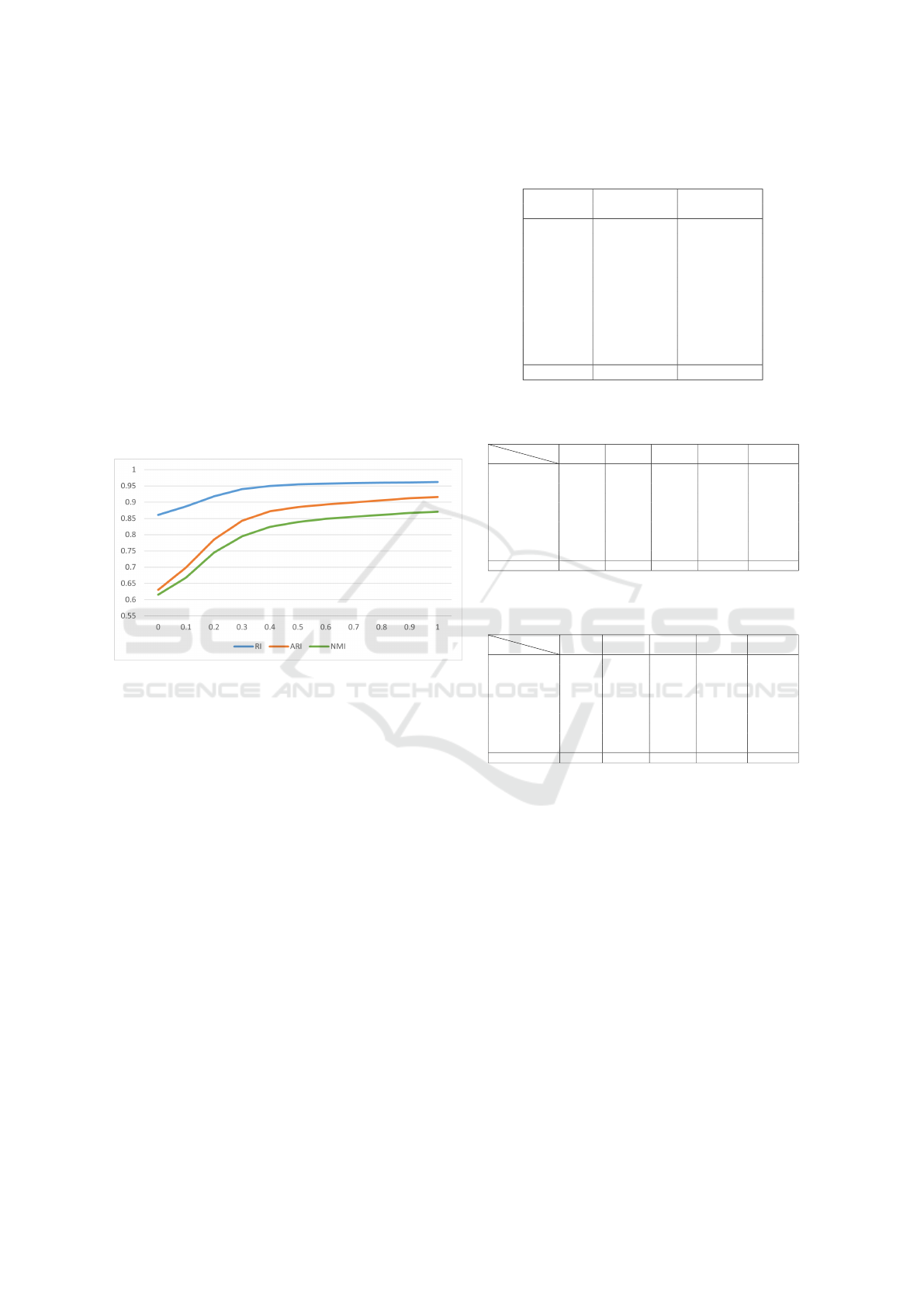
Figure 1 shows how ﬁltering segments based on con-

ﬁdence scores affects clustering metrics (RI, ARI,

and NMI, and the horizontal axis shows the thresh-

old of the conﬁdence score in the ﬁltering). As

low-conﬁdence segments are removed, the metrics

improve signiﬁcantly, indicating that segments with

lower conﬁdence are more likely to be mislabeled.

This supports the hypothesis that higher conﬁdence

scores correlate with better clustering accuracy, and

ﬁltering based on conﬁdence can enhance clustering

performance.

Figure 1: Impact of conﬁdence score ﬁltering on clustering

performance metrics for the ”Symbols” dataset.

6.3 Runtime Analysis

The performance of clustering algorithms is critical

not only in terms of accuracy but also computational

efﬁciency, especially with large datasets. In this sec-

tion, the runtime of the adapted COP-KMeans al-

gorithm is evaluated under varying conditions, com-

paring its performance with and without basepoints.

These comparisons help assess the algorithm’s scala-

bility and applicability to large scale datasets.

Table 3 compares runtimes for two conﬁgurations:

with 50 basepoints and without basepoints, all tested

on 1,000 segments. This reveals the computational

trade-offs across different setups.

Table 4 presents runtimes with 1,000 segments

and varying basepoints (from 25 to 1,000), illustrat-

ing how runtime increases with more basepoints.

Table 5 presents runtime results with a ﬁxed num-

ber of basepoints (50) while varying the number of

segments (100, 500, 1,000, 5,000, 10,000), demon-

strating how runtime scales with dataset size.

In addition, Figure 2 and 3 illustrates the average

Table 3: Runtime comparison of adapted COP-KMeans

conﬁgurations with 1,000 segments.

Dataset N × B - COP N × N - COP

(mean ± std) (mean ± std)

PLN 22.8 ± 0.6 375.4 ± 12.3

NIFECG 24.1 ± 0.4 417.3 ± 11.4

UWGLX 23.1 ± 0.7 370.4 ± 11.6

UWGLAll 23.4 ± 0.5 403.0 ± 10.0

EOGHS 23.2 ± 0.5 387.6 ± 12.2

PPTW 22.3 ± 0.3 382.9 ± 7.5

SLF 22.1 ± 0.7 374.9 ± 6.4

SYM 23.3 ± 0.7 400.8 ± 6.4

CAR 21.3 ± 0.6 363.9 ± 7.3

INSK 22.9 ± 0.4 404.0 ± 7.6

Average 22.8 ± 0.5 388.0 ± 9.3

Table 4: Runtime results with varying numbers of base-

points at a ﬁxed dataset size of 1,000 segments.

Dataset

25 50 100 200 500

PLN 11.1 ± 0.6 23.7 ± 0.4 54.5 ± 0.5 142.7 ± 0.6 615.2 ± 0.7

NIFECG 11.6 ± 0.4 24.7 ± 0.3 56.9 ± 0.4 150.6 ± 0.4 659.4 ± 0.5

UWGLX 11.4 ± 0.7 23.9 ± 0.4 55.1 ± 0.4 142.6 ± 0.5 617.0 ± 0.6

UWGLAll 11.6 ± 0.5 23.8 ± 0.5 54.9 ± 0.4 146.6 ± 0.5 642.1 ± 0.5

EOGHS 11.3 ± 0.5 23.8 ± 0.4 54.1 ± 0.4 143.4 ± 0.5 630.5 ± 0.4

PPTW 11.4 ± 0.3 22.7 ± 0.4 51.4 ± 0.4 140.6 ± 0.5 617.8 ± 0.5

SLF 10.6 ± 0.7 23.0 ± 0.5 52.4 ± 0.4 140.9 ± 0.5 623.0 ± 0.5

SYM 11.8 ± 0.7 24.2 ± 0.3 54.0 ± 0.4 144.8 ± 0.5 622.3 ± 0.6

CAR 10.6 ± 0.6 22.1 ± 0.2 51.5 ± 0.5 138.0 ± 0.4 620.4 ± 0.4

INSK 11.1 ± 0.4 23.5 ± 0.4 54.9 ± 0.4 145.2 ± 0.4 636.6 ± 0.5

Average 11.3 ± 0.5 23.5 ± 0.4 54.0 ± 0.4 143.5 ± 0.5 628.4 ± 0.5

Table 5: Runtime results with a ﬁxed number of basepoints

(50) and varying numbers of segments.

Dataset

100 500 1000 5000 10000

PLN 6.4 ± 0.6 14.6 ± 0.4 23.7 ± 0.4 96.5 ± 0.5 197.3 ± 0.6

NIFECG 6.3 ± 0.4 15.6 ± 0.3 24.7 ± 0.3 106.7 ± 0.4 199.8 ± 0.5

UWGLX 6.3 ± 0.7 14.4 ± 0.4 23.9 ± 0.4 96.0 ± 0.5 190.8 ± 0.6

UWGLAll 6.4 ± 0.5 14.9 ± 0.5 23.8 ± 0.5 101.6 ± 0.5 190.6 ± 0.5

EOGHS 6.4 ± 0.5 14.7 ± 0.5 23.8 ± 0.4 100.2 ± 0.5 192.4 ± 0.5

PPTW 6.3 ± 0.3 14.2 ± 0.4 22.7 ± 0.4 94.7 ± 0.5 178.2 ± 0.5

SLF 6.4 ± 0.7 14.4 ± 0.5 23.0 ± 0.5 96.1 ± 0.5 180.6 ± 0.5

SYM 6.4 ± 0.7 14.7 ± 0.3 24.2 ± 0.4 100.5 ± 0.5 184.8 ± 0.5

CAR 6.4 ± 0.6 13.9 ± 0.2 22.1 ± 0.5 92.5 ± 0.4 178.5 ± 0.4

INSK 6.4 ± 0.4 15.2 ± 0.4 23.5 ± 0.4 97.4 ± 0.4 188.5 ± 0.5

Average 6.4 ± 0.5 14.5 ± 0.4 23.4 ± 0.4 98.7 ± 0.5 188.5 ± 0.5

runtime of the adapted COP-KMeans algorithm as the

number of segments (n) and basepoints (b) vary. The

algorithm’s complexity is O(b · n · L · logL + b

· n +

n · b · k · I), indicating linear scaling with respect to n

and power function behavior with respect to b. The

plots conﬁrm these trends, aligning with theoretical

expectations for runtime behavior.

6.4 Sensitivity Analysis with Noise

In real-world scenarios, time series data often con-

tains noise from environmental factors or measure-

ment errors. Evaluating a clustering method under

noisy conditions is essential to assess its stability and

reliability. By introducing noise and analyzing the im-

pact on clustering performance, we can identify both

the strengths and limitations of the method, providing

a basis for potential improvements.

ICPRAM 2025 - 14th International Conference on Pattern Recognition Applications and Methods

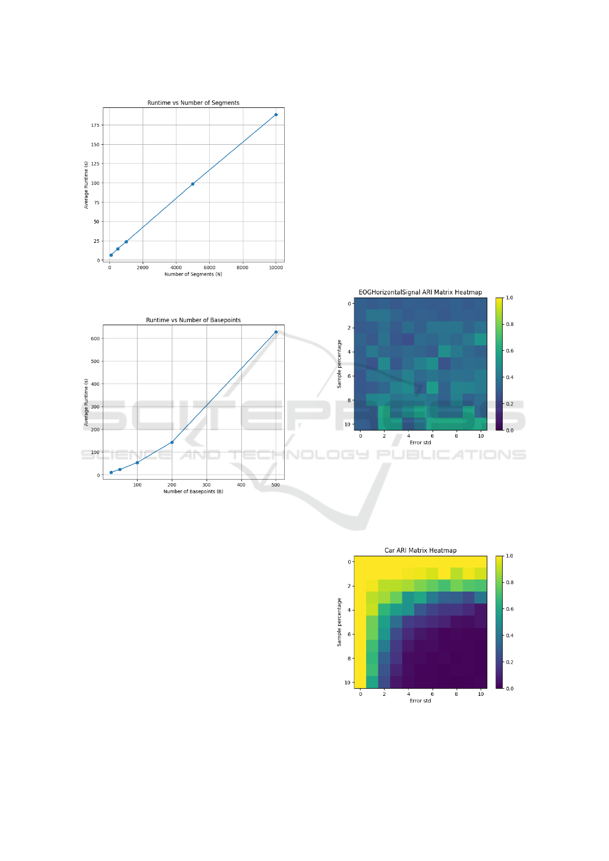
Figure 2: Average runtime of the adapted COP-KMeans al-

gorithm based on varying segments (n).

Figure 3: Average runtime of the adapted COP-KMeans al-

gorithm based on varying basepoints (b).

6.4.1 Noise Injection Strategy

To measure the sensitivity of the clustering method,

Gaussian noise is systematically injected into seg-

ments, simulating real-world sensor data imperfec-

tions. Noise is controlled by two parameters:

• Error Percentage: Deﬁnes the proportion of data

points affected by noise (e.g., 10% means 10% of

the segment is modiﬁed).

• Error Standard Deviation: Determines the magni-

tude of Gaussian noise, which has a mean of 0 and

a standard deviation ranging from 0 to 1, relative

to the segment’s data range.

Noise is incrementally applied, with both parameters

varying from 0% to 100% in 10% steps, allowing per-

formance analysis under different noise levels.

6.4.2 Results

We evaluated the impact of noise on clustering per-

formance using 11x11 ARI heatmaps, where the x-

axis represents the error standard deviation and the

y-axis indicates the sample percentage affected by

noise. The adapted COP-KMeans was run 10 times

for each conﬁguration, with results averaged for ac-

curacy. The results fall into three main categories:

1. Low Performance Without Noise: In some

datasets, the clustering method struggles even

without noise, indicated by low ARI values across

all noise levels. Noise slightly worsens results, but

the method already fails to cluster effectively (see

Figure 4).

Figure 4: EOGHorizontalSignal dataset’s ARI heatmap.

2. High Sensitivity to Noise: Some datasets show

high clustering accuracy without noise, but per-

formance rapidly degrades as noise increases.

ARI values drop to near zero, highlighting the

method’s vulnerability to noise (see Figure 5).

Figure 5: Car dataset’s ARI heatmap.

Distribution Controlled Clustering of Time Series Segments by Reduced Embeddings

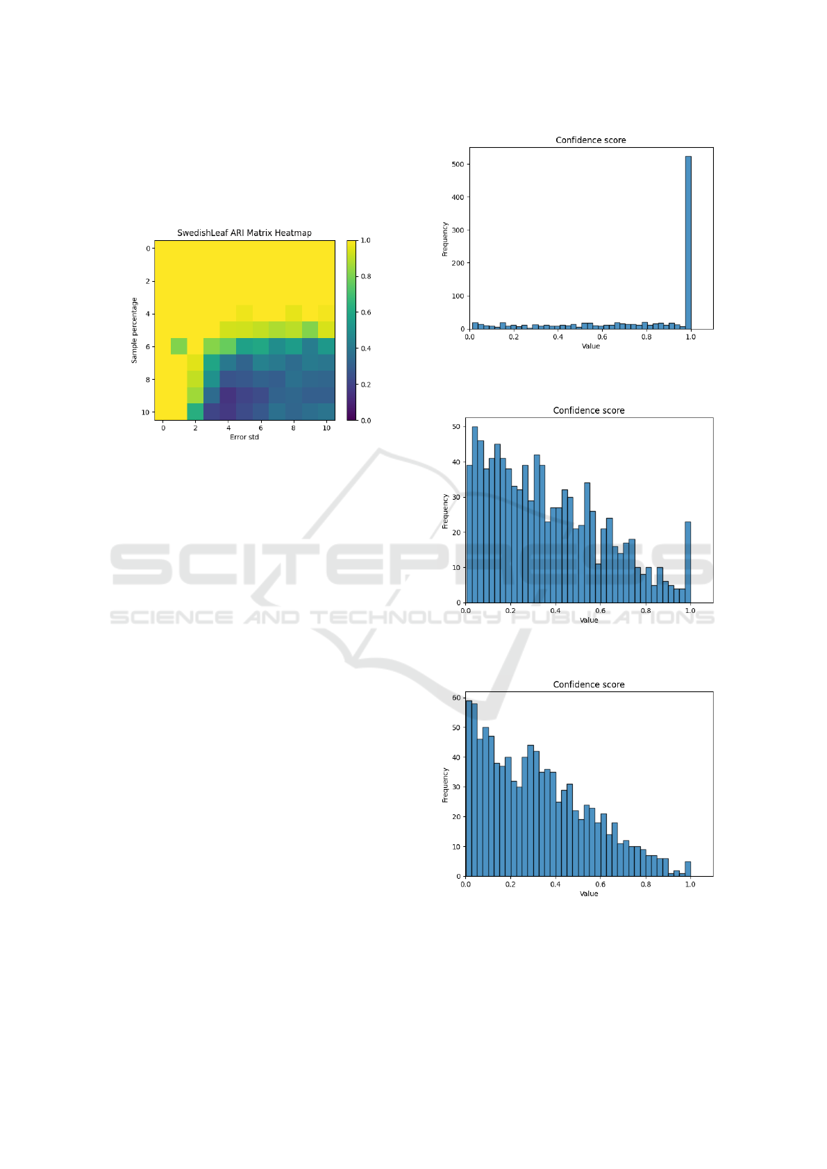
3. Moderate Sensitivity to Noise: Other datasets

maintain moderate accuracy as noise is intro-

duced. While ARI values decline, the method still

produces reasonable clusters, demonstrating some

resilience to noise (see Figure 6).

Figure 6: SwedishLeaf dataset’s ARI heatmap.

This analysis underscores the method’s varying

sensitivity to noise, suggesting areas for improvement

in noisy environments.

6.5 Conﬁdence Score Analysis

In addition to evaluating ARI values, we analyzed the

conﬁdence scores assigned to each segment. As noise

increases, the distribution of conﬁdence scores shifts

toward zero, indicating decreased reliability in clus-

tering.

6.5.1 Conﬁdence Score Distribution with

Increasing Noise

We examined the Car dataset with three noise levels:

• Low noise: At 20% noise, conﬁdence scores re-

main high for most segments, indicating reliable

clustering (see Figure 7).

• Moderate noise: At 40% noise, the distribution

shifts, with more segments receiving lower conﬁ-

dence scores, suggesting difﬁculties in differenti-

ating segments (see Figure 8).

• High noise: At 100% noise, conﬁdence scores

drop signiﬁcantly, with most values near zero,

highlighting the method’s struggle under high

noise conditions (see Figure 9).

Figure 7: Car dataset’s conﬁdence distribution with 20%

noise.

Figure 8: Car dataset’s conﬁdence distribution with 40%

noise.

Figure 9: Car dataset’s conﬁdence distribution with 100%

noise.

6.5.2 Impact of Conﬁdence Score Threshold on

Clustering Metrics

With 40% noise, increasing the conﬁdence score

threshold from 0 to 1 improves clustering metrics (RI,

ICPRAM 2025 - 14th International Conference on Pattern Recognition Applications and Methods

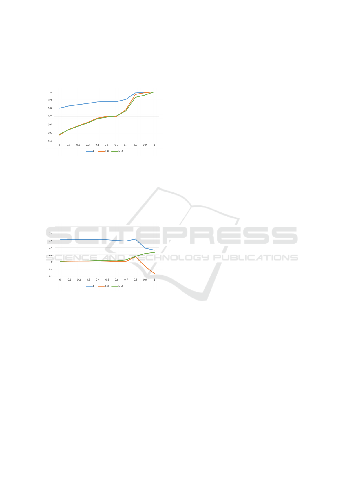
ARI, and NMI), but at the cost of discarding many

segments. This presents a trade-off between main-

taining higher conﬁdence and retaining more data, as

shown in Figure 10.

Figure 10: Impact of conﬁdence score ﬁltering on clustering

performance metrics for the ”Car” dataset with 40% noise.

At 100% noise, this trend reverses; metrics do not

improve as conﬁdence thresholds rise due to signif-

icant data loss. This illustrates that while ﬁltering

by conﬁdence enhances performance with moderate

noise, it becomes less effective in high-noise scenar-

ios, as demonstrated in Figure 11.

Figure 11: Impact of conﬁdence score ﬁltering on clustering

performance metrics for the ”Car” dataset with 100% noise.

7 CONCLUSION

In this paper, we presented a novel approach for clus-

tering time-varying segments by integrating statisti-

cal methods with constrained clustering techniques.

The primary contributions of this work include the

development of a hybrid clustering framework that

combines the Kolmogorov–Smirnov (KS) test and

adapted COP-KMeans for clustering with temporal

constraints. This approach addresses several key chal-

lenges in time series clustering, such as segment mis-

alignment, varying lengths.

The core innovation lies in using the KS test

statistic to generate distribution-based embeddings

that capture statistical differences between segments.

These embeddings provide a stable representation of

the data, independent of temporal misalignment and

length variation. Adapted COP-KMeans is then ap-

plied with cannot-link constraints, ensuring that con-

secutive segments are assigned to different clusters,

preserving their temporal structure.

To improve computational efﬁciency, we intro-

duced a basepoint selection strategy, reducing the di-

mensionality of the embedding space from O(n

) to

O(n · b). This effectively decreases the computational

complexity of the KS-based embedding construction

from O(n

· LlogL) to O(n · b · LlogL), where n is the

number of segments, b is the number of selected base-

points, and L is the segment length. The experimen-

tal results demonstrate that this basepoint reduction

signiﬁcantly enhances runtime performance without

a substantial loss in clustering accuracy (with about

10% goodness reduction, a 17-times speed-up could

be achieved). This efﬁciency gain is crucial for large

scale industrial datasets, where the traditional exhaus-

tive pairwise comparison would be computationally

prohibitive.

In addition to the basepoint strategy, we intro-

duced a conﬁdence score metric that quantiﬁes the

reliability of clustering assignments based on the rel-

ative distances to the nearest and second-nearest clus-

ter centroids. This score provides a nuanced view of

the clustering results, allowing low-conﬁdence labels

to be ﬁltered out, thus improving the overall quality

of the clustering.

The performance of our method was evaluated on

a diverse set of benchmark time series datasets, in-

cluding motion data and physiological signals. We

measured clustering performance using Rand Index

(RI), Adjusted Rand Index (ARI), and Normalized

Mutual Information (NMI). The results demonstrate

that our approach consistently outperforms traditional

clustering techniques in terms of computational efﬁ-

ciency. Furthermore, the conﬁdence-based ﬁltering

method provided a marked improvement in clustering

quality by discarding low-conﬁdence assignments.

While our proposed method shows strong perfor-

mance across multiple datasets, several avenues for

future research remain open. First, the use of alterna-

tive statistical tests and distance measures could en-

hance the sensitivity of the embedding space. The

incorporation of more sophisticated alignment tech-

niques, such as shape-based clustering methods or

Dynamic Time Warping (DTW) (M

uller, 2007), could

further improve the accuracy of our approach. Sec-

ond, while the basepoint selection strategy signiﬁ-

cantly reduces the dimensionality of the embeddings,

optimizing the selection process remains an area for

Distribution Controlled Clustering of Time Series Segments by Reduced Embeddings

further exploration.

In conclusion, the proposed framework provides

a scalable, and interpretable solution to time series

clustering, combining statistical rigour with computa-

tional efﬁciency. Our method offers a signiﬁcant step

forward in addressing the challenges of temporal mis-

alignment, variable segment lengths, and large dataset

scalability in time series clustering. By balancing the

theoretical rigour of statistical tests with the practical

demands of large scale data analysis, this work sets

the stage for future advancements in time series clus-

tering methodologies.

ACKNOWLEDGEMENTS

Project no. KDP-IKT-2023-900-I1-

00000957/0000003 has been implemented with

the support provided by the Ministry of Culture and

Innovation of Hungary from the National Research,

Development and Innovation Fund, ﬁnanced under

the C2299763 funding scheme.

REFERENCES

Aghabozorgi, S., Shirkhorshidi, A. S., and Wah, T. Y.

(2015). Time-series clustering–a decade review. In-

formation systems, 53:16–38.

Anderson, T. W. and Darling, D. A. (1952). Asymptotic

Theory of Certain ”Goodness of Fit” Criteria Based

on Stochastic Processes. The Annals of Mathematical

Statistics, 23(2):193 – 212.

Arthur, D. and Vassilvitskii, S. (2007). K-means++: the

advantages of careful seeding. In Proc. of the 18th an-

nual ACM-SIAM symposium on Discrete algorithms,

page 1027–1035. SIAM, Philadelphia, PA, USA.

Caiado, J., Maharaj, E. A., and D’Urso, P. (2015). Time

series clustering. In Handbook of Cluster Analysis,

pages 241–263. CRC Press.

Ermshaus, A., Sch

afer, P., and Leser, U. (2023). Clasp:

parameter-free time series segmentation. Data Mining

and Knowledge Discovery, 37(3):1262–1300.

Ertl, B., Meyer, J., Schneider, M., and Streit, A. (2021).

Semi-supervised time point clustering for multivari-

ate time series. In The 34th Canadian Conference on

Artiﬁcial Intelligence. Springer.

Fujimaki, R., Hirose, S., and Nakata, T. (2008). Theoretical

analysis of subsequence time-series clustering from a

frequency-analysis viewpoint. In International Con-

ference on Data Mining, pages 506–517. SIAM.

Guijo-Rubio, D., Dur

an-Rosal, A. M., Guti

errez, P. A.,

Troncoso, A., and Herv

as-Mart

ınez, C. (2021). Time-

series clustering based on the characterization of seg-

ment typologies. IEEE Transactions on Cybernetics,

51(11):5409–5422.

Hautamaki, V., Nykanen, P., and Franti, P. (2008). Time-

series clustering by approximate prototypes. In

19th International Conference on Pattern Recogni-

tion, pages 1–4. IEEE.

Hubert, L. J. and Arabie, P. (1985). Comparing partitions.

Journal of Classiﬁcation, 2:193–218.

Keogh, E. and Lin, J. (2005). Clustering of time-series sub-

sequences is meaningless: implications for previous

and future research. Knowledge and Information Sys-

tems, 8:154–177.

Kolmogorov, A. (1933). Sulla determinazione empirica di

una legge di distribuzione. Giornale dell’Istituto Ital-

iano degli Attuari, 4:83.

Li, Y., Lin, J., and Oates, T. (2012). Visualizing variable-

length time series motifs. In Proceedings of the

2012 SIAM International Conference on Data Mining,

pages 895–906. SIAM.

Li, Y., Shen, D., Nie, T., and Kou, Y. (2022). A new shape-

based clustering algorithm for time series. Informa-

tion Sciences, 609:411–428.

Liao, T. W. (2005). Clustering of time series data—a survey.

Pattern Recognition, 38(11):1857–1874.

Meesrikamolkul, W., Niennattrakul, V., and Ratanama-

hatana, C. A. (2012). Shape-based clustering for time

series data. In Advances in KDDM: 16th Paciﬁc-Asia

Conference, PAKDD, Kuala Lumpur, Malaysia, May

29-June 1, 2012, Part I, pages 530–541. Springer.

orchen, F., Ultsch, A., and Hoos, O. (2005). Extract-

ing interpretable muscle activation patterns with time

series knowledge mining. International Journal of

Knowledge-based and Intelligent Engineering Sys-

tems, 9(3):197–208.

uller, M. (2007). Dynamic Time Warping, pages 69–84.

Springer.

Rakthanmanon, T., Campana, B., Mueen, A., Batista, G.,

Westover, B., Zhu, Q., and Keogh, E. (2013). Ad-

dressing big data time series: Mining trillions of

time series subsequences under dynamic time warp-

ing. ACM Transactions on Knowledge Discovery from

Data (TKDD), 7(3):1–31.

Rakthanmanon, T., Keogh, E. J., Lonardi, S., and Evans, S.

(2012). Mdl-based time series clustering. Knowledge

and Information Systems, 33:371–399.

Rand, W. M. (1971). Objective criteria for the evaluation of

clustering methods. Journal of the American Statisti-

cal Association, 66(336):846–850.

Rodpongpun, S., Niennattrakul, V., and Ratanamahatana,

C. A. (2012). Selective subsequence time series clus-

tering. Knowledge-Based Systems, 35:361–368.

Vinh, N. X., Epps, J., and Bailey, J. (2009). Information the-

oretic measures for clusterings comparison: is a cor-

rection for chance necessary? In Proceedings of the

26th ICML, pages 1073–1080.

Wagstaff, K., Cardie, C., Rogers, S., and Schr

odl, S.

(2001). Constrained k-means clustering with back-

ground knowledge. In Proceedings of the 18th ICML,

volume 1, pages 577–584.

Yang, T. and Wang, J. (2014). Clustering unsynchronized

time series subsequences with phase shift weighted

spherical k-means algorithm. Journal of Computers,

9(5):1103–1108.

Zolhavarieh, S., Aghabozorgi, S., and Teh, Y. W. (2014).

A review of subsequence time series clustering. The

Scientiﬁc World Journal, 2014(1):312521.

ICPRAM 2025 - 14th International Conference on Pattern Recognition Applications and Methods