Partition Tree Ensembles for Improving Multi-Class Classiﬁcation

Miran

Ozdogan

1 a

, Alan Jeffares

2 b

and Sean Holden

3 c

Department of Computer Science, Oxford University, U.K.

Department of Applied Mathematics and Theoretical Physics, Cambridge University, U.K.

Department of Computer Science, Cambridge University, U.K.

Keywords:

Multi-Class Classiﬁcation, Non-Convex Optimization, AutoML.

Abstract:

We propose the Partition Tree Ensemble (PTE), a novel tree-based ensemble method for classiﬁcation prob-

lems. This differs from previous approaches in that it combines ideas from reduction methods—that decom-

pose multi-class classiﬁcation problems into binary classiﬁcation problems—with the creation of specialised

base learners that are trained on a subset of the input space. By exploiting multi-class reduction, PTEs adapt

concepts from the Trees of Predictors (ToP) method to successfully tackle multi-class classiﬁcation problems.

Each inner node of a PTE splits either the feature space or the label space into subproblems. For each node

our method then selects the most appropriate base learner from the provided set of learning algorithms. One of

its key advantages is the ability to optimise arbitrary loss functions. Through an extensive experimental eval-

uation, we demonstrate that our approach achieves signiﬁcant performance gains over the baseline ToP and

AdaBoost methods, across various datasets and loss functions, and outperforms the Random Forest method

when the label space exhibits clusters where some classes are more similar to each other than to others.

1 INTRODUCTION

Ensemble methods have gained popularity in super-

vised machine learning as a strategy for maximising

performance by aggregating the predictions of multi-

ple base learners. It is often advantageous to organ-

ise these base learners using a tree structure. Exam-

ples of such tree-based ensembles include Nested Di-

chotomies (NDs) (Frank and Kramer, 2004), Model

Trees (MTs) (Quinlan et al., 1992) and Trees of Pre-

dictors (ToPs) (Yoon et al., 2018b; Yoon et al.,

2018a).

ToPs employ tree structures to decompose classi-

ﬁcation problems. They apply distinct base learners

to various subsets of the feature space, and optimise

for arbitrary loss functions. This can be an advan-

tage, especially in the ﬁeld of healthcare where it is

often appropriate to evaluate classiﬁer performance

in terms of AUC (Cortes and Mohri, 2003) or other

non-standard measures (Yoon et al., 2018a; Beneke

et al., 2023). Yoon et al. (Yoon et al., 2018b) demon-

strated that ToPs can yield substantial performance

https://orcid.org/0009-0008-7776-6107

https://orcid.org/0009-0003-8744-0876

https://orcid.org/0000-0001-7979-1148

gains when compared to frequently utilised methods

such as Random Forests and AdaBoost (Yoon et al.,

2018b). However, their evaluation of the ToPs ap-

proach was limited to binary classiﬁcation problems.

Our preliminary experiments showed that their per-

formance compared to baselines diminishes with an

increasing number of classes.

This inspired us to devise an ensemble method

that, similarly to the ToP approach, is able to optimise

for arbitrary loss functions and overcome the short-

comings of ToPs for multi-class problems. We intro-

duce the PTE, a novel tree-based ensemble approach

that combines ideas from reduction techniques (Frank

and Kramer, 2004), which decompose multi-class

classiﬁcation problems, with the creation of spe-

cialised base learners that are trained on a subset of

the input space, as exempliﬁed by the ToP approach.

We draw inspiration from the Nested Dichotomies

(NDs) (Frank and Kramer, 2004) reduction tech-

nique, which achieves state-of-the-art performance

compared to competitors such as One-VS-One or

One-VS-Rest (Wever et al., 2023; Leathart, 2019). In

PTEs, each inner node of a PTE splits either the fea-

ture space or the label space. For the latter, we divide

the set of possible classes into two subsets that de-

ﬁne three classiﬁcation problems: “Which of the two

Özdogan, M., Jeffares, A. and Holden, S.

Partition Tree Ensembles for Improving Multi-Class Classiﬁcation.

DOI: 10.5220/0013163400003905

Paper published under CC license (CC BY-NC-ND 4.0)

In Proceedings of the 14th International Conference on Pattern Recognition Applications and Methods (ICPRAM 2025), pages 55-69

ISBN: 978-989-758-730-6; ISSN: 2184-4313

subsets does a sample belong to?” and “Given that

a sample is part of one of the subsets, which of its

classes does it belong to?”.. By exploiting such Class

Dichotomies, we can more effectively decompose the

original learning problem, and extend the advantages

of ToPs to multi-class problems.

We assess the value of this approach through an

experimental evaluation, comparing its performance

with ToPs, Random Forests and AdaBoost. Our eval-

uation employs nine datasets from the UCI reposi-

tory (Dua and Graff, 2017). In addition, we conduct

experiments on optimising for two different loss func-

tions, speciﬁcally the AUC (Cortes and Mohri, 2003)

and the F1-Measure (Chicco and Jurman, 2020).

In summary, our contributions are as follows:

• We introduce the PTE and provide a comprehen-

sive formal description of the method.

• We present a detailed mathematical derivation

of the computational complexity associated with

training PTEs.

• In an extensive experimental evaluation, we com-

pare PTEs against ToPs and additional baselines

of Random Forests (Breiman, 2001) and Ad-

aBoost (Freund et al., 1999). We are able to

show that PTEs can lead to substantial perfor-

mance gains over ToPs and AdaBoost.

2 RELATED WORK

An overview of the respective differences between

PTEs, ToPs, NDs and Model Trees can be found

in Table 1. We acknowledge that other tree-

Table 1: Comparison of PTEs with Existing Tree-Based En-

semble Methods.

Method PTE MT ND ToP

Multiple Base Learners ✔ ✘ ✘ ✔

Partition X ✔ ✔ ✘ ✔

Partition Y ✔ ✘ ✔ ✘

Non-Convex Loss ✔ ✘ ✘ ✔

Classiﬁcation ✔ ✘ ✔ ✔

Regression ✘ ✔ ✘ ✔

based ensemble methods exist, including Filter

trees (Beygelzimer et al., 2007) and Kernel Regres-

sion Tree (Torgo, 1997b). However, we will focus on

NDs, ToPs and Model Trees as these are the methods

most similar to PTEs.

Figure 1: Illustrative example of a Nested Dichotomy

with Y = {c

}. Figure adapted to our notation

from (Wever et al., 2023).

2.1 Nested Dichotomies

Nested Dichotomies (NDs) (Frank and Kramer, 2004)

are ensembles that employ a binary tree structure to

recursively break down a multi-class classiﬁcation

problem into a set of binary classiﬁcation problems.

They facilitate the application of classiﬁers that are

inherently binary to multi-class problems.

We can represent an ND as a binary tree, where

each node corresponds to a subset of classes from the

original multi-class classiﬁcation problem. The sub-

trees of a node recursively divide its set of classes into

distinct subsets, forming the meta-classes that corre-

spond to its two children until a subset contains only

a single element. At each internal node, the division

constitutes a binary classiﬁcation problem that is ad-

dressed by a base learner (Frank and Kramer, 2004).

An illustration of this method can be found in Fig-

ure 1.

Since the initial work by Frank and Kramer (Frank

and Kramer, 2004), extensive research has been

conducted on the selection of good ND structures

(Leathart, 2019). We now discuss two contemporary

state-of-the-art methods. Leathart et al. (Leathart,

2019) sought to create trees with easier binary clas-

siﬁcation problems by employing dichotomies that

group together classes that are “similar”. This method

is called Random Pair Nested Dichotomies (RPNDs).

In this approach, an initial pair of classes is ran-

domly selected. Then each of the other classes is

grouped with one of those two. The assignment of

other classes is determined by training a binary clas-

siﬁer on the initial classes. This classiﬁer is applied

to the remaining data and the remaining classes are

assigned based on the classiﬁer’s predictions through

hard voting. Note, that the binary classiﬁer employed

for class grouping is discarded, and a new binary clas-

siﬁer is trained to differentiate between the two meta-

classes. Leathart et al. (Leathart, 2019) demonstrated

that ensembles constructed using this technique ex-

hibit state-of-the-art predictive performance while be-

ing less runtime-intensive than competing methods.

Wever et al. (Wever et al., 2023) propose a co-

evolutionary algorithm CONDA aimed at discovering

advantageous ensembles of NDs. In contrast with

ICPRAM 2025 - 14th International Conference on Pattern Recognition Applications and Methods

Figure 2: Illustrative example of a Tree of Predictors.

RPNDs, this requires a comprehensive optimisation

of the entire tree structure, rather than the successive

growth of the ND tree. It demonstrates superior pre-

dictive performance when compared to RPNDs, al-

beit at the expense of a signiﬁcant increase in run-

time (Wever et al., 2023).

Interestingly, Mohr et al. (Mohr et al., 2018)

found that, for multi-class problems, implementing

partial NDs of depth 1 (referred to simply as “Di-

chotomies” in the statistical literature) can sometimes

enhance performance, when compared to using indi-

vidual base learners.

2.2 Trees of Predictors

In this section, we describe the ToPs ensemble

method as introduced in (Yoon et al., 2018a; Yoon

et al., 2018b). We will assume that categorical fea-

tures are one-hot encoded and continuous features are

normalised such that X

∈ [0, 1] for every feature j

and X ⊆ [0, 1]

. For subsets Z

⊆ X of the feature

space, if predictors h

: Z

7→ Y and h

: Z

7→ Y

are constructed such that Z

∩ Z

0, we deﬁne

∨h

: Z

∪Z

7→ Y as h

∨h

(z) = h

(z) for z ∈ Z

2.2.1 Formal Deﬁnition

A Tree of Predictors can be represented as a binary

tree, denoted T . Each node N within this tree corre-

sponds to a subset X of the feature space and is associ-

ated with a classiﬁer h

. The corresponding subset is

used interchangeably to refer to a node and vice versa.

The root node of T must corresponds to the entire fea-

ture space X . For any given node N ∈ T its children,

denoted {N

−

}, partition N. For a node N ∈ T , its

corresponding classiﬁer h

is generated by training

an algorithm A

∈ A on a set N

∗

, where N

∗

= N or

∗

corresponds to one of the predecessors of N. For-

mally, this relationship is expressed as h

= A

∗

)

with N

∗

∈ N

↑

The set of leaves, denoted T , forms a partition of

the feature space X . We denote the leaf correspond-

ing to some feature vector x ∈ X as N(x). An illus-

trative example of a Tree of Predictors is provided in

Figure 2.

Note that this approach allows for a node’s classi-

ﬁer to be trained on a set that corresponds to one of

its predecessors. This design choice is driven by the

understanding that partitioning the training set may

result in performance enhancement for one subset,

while degrading performance for another.

2.2.2 Growing a Tree of Predictors

Growing a ToP requires a ﬁnite set A = A

,. . ., A

base learner algorithms as input, as well as a training

set D and two validation sets V

and V

. The pre-

dictor that is obtained by training an algorithm A ∈ A

on some subset E ⊆ D of the training data is denoted

A(E). Let E be a collection of subsets of the training

data D. We then deﬁne A(E ) = {A(E) : A ∈ A, E ∈

E} as the set of predictors obtained from training each

algorithm in A on every set in E. Given a subset

N ⊂ X of the feature space and a subset E ⊂ D of the

dataset, we let E(N) = {(x

) ∈ E : x

∈ N}. When

provided with disjoint sets E

,. . ., E

and correspond-

ing predictors h

on E

, we denote the overall loss as

L (

The process is initialised with the root node X and

the corresponding classiﬁer h

. The classiﬁer is cho-

sen such that h

= A(D(X )), where A is selected from

the set of algorithms A such that it minimises the val-

idation loss on V

Then the children of each leaf N ∈ T are re-

cursively created. For this, the corresponding fea-

ture space is split along the feature i and threshold

∈ [0,1] that result in the best validation loss mea-

sured on V

. We write

−

= {x ∈ N : x

< τ

},N

= {x ∈ N : x

≥ τ

} (1)

In practice, for each continuous feature up to 9 can-

didate thresholds are selected at the 10th, 20th, ...,

90th percentiles. For every candidate threshold τ

the predictors h

−

∈ A(N

−↑

), h

∈ A(N

+↑

) are cho-

sen such that they minimise the validation loss where

↑

to denotes the set consisting of node N and all its

predecessors that correspond to the same label space.

From these predictors we then determine h

−

∗

, h

∗

that minimise the total validation loss.

A node N is only split if its loss is strictly higher

than the total loss of its children N

−

and N

. The

pseudo-code for this can be found in Algorithm 1.

2.2.3 Weighting Predictors for Optimal

Predictions

Once the locally optimal tree is established, the next

step is to determine how to weight the various pre-

dictors. The prediction for a sample x is determined

by the sequence of nodes

∏

, which spans the path

from the root node to the leaf node N(x) that corre-

Partition Tree Ensembles for Improving Multi-Class Classiﬁcation

Algorithm 1: Growing the Optimal Tree of Predic-

tors. Adapted from (Yoon et al., 2018b).

Require: Feature space X , set of algorithms A,

training set D, ﬁrst validation set V

← arg min

h∈A(D)

L(h,V

)

T ← (X , h

Recursive step:

Input: Current Tree of Predictors T

for each leaf N ∈ T do

for each feature i and threshold τ

−

← {x ∈ N : x

< τ

}

← {x ∈ N : x

≥ τ

}

end

let h

−

∈ A(N

−

), h

∈ A(N

)

⋆

,τ

⋆

−

) ←

argminL



−

∨ h

(N)



end

Stopping criterion:

L(h

(N)) ≤

min



−

∨ h

−

) ∪V

)



sponds to x. Each leaf node is assigned an individ-

ual weight vector ⃗w = (w

)

N∈

∏

, which deﬁnes the

weights of predictors corresponding to nodes on the

root-leaf path. These weights are used to generate

predictions for samples associated with N(x). The en-

tire weight vector of a leaf is individual; that is, the

common ancestor of two leaves might have different

weights assigned by them.

Weights are required to be non-negative and sum

to one. For each leaf, weight vectors are chosen by

utilising linear regression to minimise the empirical

loss on the corresponding subset of the second vali-

dation set V

(N(x)).

2.3 Model Trees

Model Trees (Quinlan et al., 1992), are a tree-based

ensemble method for solving regression tasks. They

combine a conventional Decision Tree structure with

the possibility of linear regression functions at the leaf

nodes (Wang and Witten, 1997).

In the ﬁrst phase of Model Tree construction, a

Decision Tree induction algorithm (Breiman et al.,

1984) is employed. As a splitting criterion it min-

imises the variation in class values within each sub-

set across the branches. During the second phase, it

prunes the tree, starting from each leaf and working

upwards. This aims to reduce overﬁtting by removing

or replacing less informative nodes (Breiman et al.,

1984; Quinlan, 1986). A key distinction from conven-

tional pruning methods is that, when pruning back to

an internal node, the method involves replacing that

node with a regression plane rather than a constant

value (Wang and Witten, 1997).

Several works have expanded on the original

Model Tree method. Torgo (Torgo, 1997a) introduced

an approach that allows for different models within

the leafs of the tree. However, Torgo’s method re-

mains constrained to growing the tree based on a sin-

gle base learner. Malerba et al. (Malerba et al., 2001)

proposed a Model Tree induction algorithm that has

some similarities with our PTE method. It employs a

splitting criterion based on how well linear models ﬁt

the data at a node during tree growth.

2.3.1 Differences to Partition Tree Ensembles

Primarily, Model Trees are designed to address re-

gression tasks, whereas PTEs are designed for clas-

siﬁcation problems. Additionally, PTEs do not utilise

pruning or smoothing techniques. Instead, they em-

ploy Stacked Generalisation (Wolpert, 1992) to deter-

mine the weights assigned to models along the path

from the root to the leaf node. Furthermore, Model

Trees solely partition the feature space, whereas PTEs

have the versatility to partition both the feature space

and the label space.

Importantly, Model Trees are induced using a sin-

gle base learner algorithm while PTEs provide the

ﬂexibility to select the most suitable base learner at

each tree node.

Lastly, Model Trees are restricted to using convex

loss functions (Yoon et al., 2018b). This can be disad-

vantageous when optimising for F-score or AUC, as is

frequently done in medical applications. In contrast,

PTEs offer the ﬂexibility to optimise non-convex loss

functions.

3 PARTITION TREE ENSEMBLES

In this section, we introduce PTEs. First, in Sec-

tion 3.1 we explain the motivation for this method.

Then in Section 3.2 we formally introduce Class Di-

chotomies, which constitute the inner nodes of Nested

Dichotomies. (Note that in the statistical literature

these are referred to simply as “Dichotomies”.) In-

spired by (Leathart et al., 2016) we use the Random

Pair method to select Class Dichotomies for PTEs.

We describe this in Section 3.3. In Section 3.4 we

provide a formal deﬁnition of PTEs. Then, in Sec-

tion 3.5 we describe our method for inducing them.

Finally, in Section 3.6 we describe how we aggregate

base learner predictions into an overall prediction.

ICPRAM 2025 - 14th International Conference on Pattern Recognition Applications and Methods

3.1 Motivation

In this section, we succinctly present the motivation

underpinning our PTE algorithm. Previous work by

Yoon et al. (Yoon et al., 2018b) highlighted how a

Tree of Predictors can produce signiﬁcant improve-

ments over baseline methods such as AdaBoost, and

Random Forest. However, their experimental anal-

ysis was conﬁned to binary classiﬁcation datasets.

Our preliminary experiments applying ToPs to multi-

class classiﬁcation problems revealed that their per-

formance advantage over the baselines diminishes

with a higher number of classes.

Achieving high performance in terms of loss func-

tions other than the cross-entropy loss can be piv-

otal, especially in healthcare applications. Conven-

tional performance measures such as cross-entropy

loss or accuracy are often not the most suitable met-

rics in medical settings (Yoon et al., 2018a). In many

cases, employing other loss functions such as AUC-

Loss (Cortes and Mohri, 2003) or the F-Measure (Gu

et al., 2009) may be more appropriate. Hence, our

goal was to identify an ensemble method compara-

ble to Tree of Predictors, which can successfully opti-

mise arbitrary loss functions for multi-class problems

as well.

In response to this challenge, we present PTEs.

Like ToPs, PTEs recursively split the classiﬁcation

problem into subproblems associated with the nodes

of a binary tree. However, in addition to splitting

the feature space, nodes within the tree can parti-

tion the label space using Class Dichotomies, thereby

giving rise to sub-problems derived from the initial

multi-class classiﬁcation problem. Since these sub-

problems have a lower number of classes compared

to the original problem, we are able to obtain perfor-

mance gains similar to those we observed for ToPs in

binary classiﬁcation problems.

3.2 Class Dichotomies

In this section, we provide a formal deﬁnition of

Class Dichotomies, which serve as a means to par-

tition a multi-class classiﬁcation problem into three

distinct sub-problems. Class Dichotomies are utilised

at every inner node of a ND tree. In early ma-

chine learning literature, the individual nodes of

a Nested Dichotomy were themselves referred to

as Nested Dichotomies (Frank and Kramer, 2004).

However, in contemporary usage, the term “Nested

Dichotomies” has evolved to encompass the entire

tree structure (Leathart, 2019).

Given a classiﬁcation problem with Y =

,. . ., c

}, a Class Dichotomy partitions the set of

classes into two subsets. Without loss of general-

ity, let these subsets be Y

−

= {c

,. . ., c

} and Y

j+1

,. . ., c

}. It is important to note that Class Di-

chotomies may deﬁne arbitrary non-empty partitions,

and the ordering of classes is not relevant to this. To

construct a predictor that addresses the original multi-

class problem, the Class Dichotomy combines predic-

tions for three sub-problems, which are deﬁned by the

two subsets. First, the Class Dichotomy includes a

predictor h

−

that differentiates between the two

meta-classes determined by Y

−

and Y

. This means

that, for a given sample (x,y), h

−

(x) estimates

the probability p(y ∈ Y

−

|x). Also, the Class Di-

chotomy has two predictors, h

−

and h

, which es-

timate the class probabilities of a sample, assuming

it belongs to the respective subset; that is, h

esti-

mates p(y = c

|x,y ∈ Y

) for all classes c

∈ Y

where

∈ {Y

−

}. We can simply multiply the condi-

tional probability with the probability of its condition

to obtain an overall class probability estimate:

p(y = c

|x) = p(y = c

|x,c

∈ Y

) · p(c

∈ Y

|x) (2)

Thus, for each class c

∈ Y

, if Y

= Y

−

, we can

estimate p(y = c

|x) using h

−

(x) · h

−

(x), and if

= Y

, using



1 − h

−

(x)



· h

(x). We refer

to this overall classiﬁer as h

3.3 Random Pair Method

Inspired by (Leathart et al., 2016), we propose the

use of the Random Pair method to generate Class

Dichotomies within our PTEs. Our rationale is as

follows: among methods that rely on iterative split-

ting, RPNDs have demonstrated the best performance

in selecting NDs (Leathart, 2019). Although this

may not directly translate to optimal performance for

choosing individual Class Dichotomies, we believe it

serves as a good proxy. In this section, we present

a detailed explanation of the method along with the

corresponding pseudocode.

The process begins by randomly selecting two

classes, c

−

and c

, from the label space Y without

replacement. Following this, we utilise the available

training data for these classes to train a binary clas-

siﬁer h

−

to distinguish between the two classes.

This classiﬁer is applied to the remaining training

data and the remaining classes are assigned to one

of two sets Y

−

based on the classiﬁer’s predic-

tions through hard voting. Speciﬁcally, if the classi-

ﬁer predicts that the majority of data points belonging

to class c

are in class c

−

, class c

will be allocated

to the subset Y

−

surrounding c

−

. Otherwise, it will

be assigned to the subset Y

. Once the two meta-

classes Y

−

and Y

are formed, we discard h

−

Partition Tree Ensembles for Improving Multi-Class Classiﬁcation

and train a new classiﬁer h

−

using the training

set {(x,0)|(x,y) ∈ D, y ∈ Y

−

}∪ {(x,1)|(x, y) ∈ D, y ∈

} to distinguish between the two meta-classes. To

form a complete Class Dichotomy, we also train and

select h

−

= argmin

A∈A



A(D

−

),V

−



and h

argmin

A∈A



A(D

),V



which constitute the opti-

mal models for the two respective sub-problems.

We choose this method to create Class Di-

chotomies because it has been used to develop state-

of-the-art NDs (Leathart et al., 2016). Although evo-

lutionary algorithms NDEA (Wever et al., 2018) and

CONDA (Wever et al., 2023) have recently outper-

formed RPNDs, these methods optimise the entire

ND tree instead of individual dichotomies. Conse-

quently, they are not suitable for our purposes.

3.4 Formal Deﬁnition

In this section, we provide a formal introduction to the

PTE method. We employ the same notation as in Sec-

tion 2.2, and we continue to assume that categorical

features are represented in binary form and continu-

ous features are normalised. For our PTE method, we

require a ﬁnite set of m candidate algorithms, denoted

as A = {A

,. . ., A

}, as well as a set of m

candi-

date algorithms A

that we use to create predictors

which distinguish between the meta-classes in Class

Dichotomies.

Each node N within this tree corresponds to a sub-

set of the feature space X

⊆ X and a subset of the

label space Y

⊆ Y . A classiﬁer h

is associated

with each node, mapping the feature space to the re-

spective subset of the label space. It is generated by

training an algorithm A

∈ A on a subset of the fea-

ture space corresponding to node N

∗

, where N

∗

either N or one of its predecessors that corresponds

to the same subset of the label space Y

. Formally,

this relationship is expressed as h

= A

∗

) where

∗

∈ N

∗

↑)∧(Y

∗

= Y

). For any given node N ∈ T ,

its children, denoted as {N

−

}, partition the lo-

cal feature space X

and correspond to the local label

space Y

or vice versa. If and only if a node’s suc-

cessors split the label space, it contains an additional

predictor h

−

that is generated by training an al-

gorithm A

∈ A

to distinguish between the two

meta-classes deﬁned by the subsets Y

−

and Y

To grow a Partition Tree, we randomly partition

the available dataset into the training set D and two

validation sets V

and V

. Given a subset of the feature

space N ⊂ X and a subset of the dataset Z ⊂ D, we

let Z(N) = {(x

) ∈ Z : x

∈ N}. Our general model

accommodates the optimisation of arbitrary loss func-

tions. An illustrative example of a PTE is provided in

Figure 3.

Figure 3: Illustrative example of a Partition Tree Ensemble

with Y = {c

3.5 Growing a Partition Tree

In this subsection, we introduce our algorithm for

growing Partition Trees, building upon the algorithm

for growing ToPs from Section 2.2. This extension

enables splits of the label space, utilising the concept

of Class Dichotomies introduced earlier.

Similarly to the procedure for growing ToPs, we

begin with the trivial Partition Tree containing only

the root node corresponding to (X ,Y ). When creat-

ing children for each node, we ﬁrst estimate the op-

timal split of the feature space, as for ToPs. Instead

of immediately generating the children based on this

optimal split, we further create a candidate Class Di-

chotomy for each A

∈ A

. For this purpose, we

utilise the Random Pair method, as outlined in Sec-

tion 3.3, to create two meta-classes. Then, the al-

gorithm A

is trained on these meta-classes, yield-

ing h

−

. Using the validation set V

, we select

the optimal algorithms A

−

∈ A to create h

−

and

. These three predictors collectively form h

Y ,CD

The optimal h

∗

Y ,CD

is chosen from the m

Class Di-

chotomies created in this manner, based on the valida-

tion set V

. If h

∗

Y ,CD

demonstrates a lower loss com-

pared to the optimal split of the feature space, then

we create the node’s children based on this Class Di-

chotomy instead of splitting the feature space. In this

case, the children will correspond to partitions of the

local label space Y

−

and Y

, while sharing the same

local feature space. Additionally, the current node

will be assigned the meta-classiﬁer h

−

, which is

used to combine the predictions of its children. This

recursive process of creating the children’s offspring

continues until neither the best Class Dichotomy nor

the optimal feature space split can further improve

the local loss. The pseudocode for PTEs is in Algo-

rithm 2.

If a node’s children partition the label space, it is

necessary to assign them a new second validation set

. To achieve this, we split off a new validation set

from the training set at the current node and pass it to

the children as the V

set. This step is crucial because,

ICPRAM 2025 - 14th International Conference on Pattern Recognition Applications and Methods

Algorithm 2: Growing the Optimal Partition Tree

Ensemble.

Require: Training set D, the ﬁrst validation set

, a set of base estimators A, a set of binary

base estimators for Class Dichotomies A

← argmin

A∈A

L(A(D);V

)

root ← (X ,h

Recursive step:

Require: node (N,h

) for a feature i and a

threshold τ

−

← {x ∈ N : x

< τ

}

← {x ∈ N : x

≥ τ

}

end

let h

−

∈ A(D(N

−

)), h

∈ A(D(N

)) :

⋆

,τ

⋆

−

) ← arg min L



−

∪ h

(N)



← randomPair(D(N),V

(N),A, A

)

← L(h

−

⋆

∪ h

⋆

(N))

← L (h

(N)))

← L (h

(N))

if (L

< L

) ∧ (L

≤ L

) then

node.le f t ← (N

−

⋆

)

node.right ← (N

⋆

)

recurse(node.le f t)

recurse(node.right)

end

if (L

< min(L

) then

node.CD ← h

recurse(node.CD.le f t)

recurse(node.CD.right)

end

Stopping criterion:

≤ min(L

)

without it, stacking would be biased towards assign-

ing higher weights to predictions resulting from Class

Dichotomies. The reason for this will become more

clear in the next section.

3.6 Weighting and Assembling

Predictions

In PTEs, we cannot assemble predictions in the same

manner as in ToPs. This is because base learners be-

low a Class Dichotomy are trained on a sub-problem

with fewer classes. Therefore, integrating their pre-

dictions into the original multi-class problem requires

the use of predictor h

−

, which has been trained

on the meta-classes at the Class Dichotomy node.

To tackle this, we conceptually regard nodes con-

taining a Class Dichotomy as leaf nodes, and their

subtrees as independent PTEs. This strategy enables

us to integrate the two subtrees and the meta-classiﬁer

at a Class Dichotomy into a single predictor h

Consequently, our tree now resembles a tree of pre-

dictors, with the exception that we have an added

predictor h

at each leaf node containing a Class

Dichotomy. We can then employ linear regression

to deﬁne a weight vector ⃗w, allocating non-negative

weights to each of the predictors on the path from the

root to the leaf node, including the additional h

However, to make this feasible, the subtrees of the

Class Dichotomy must be functional PTEs, implying

that weight vectors must have already been assigned

to them. Therefore, we initiate this process at the low-

est Class Dichotomies and work our way up the tree.

Now, the need for creating new V

sets for the chil-

dren at nodes with Class Dichotomies becomes appar-

ent. If we use the same validation set V

to assign the

weight vectors to the children, the estimated perfor-

mance of h

on V

will be biased, and the weight

assigned to it will likely be higher than optimal.

4 IMPLEMENTATION

We implement PTEs in Python 3.11.1 and adhere

to the guidelines for developing scikit-learn estima-

tors (Pedregosa et al., 2011).

In our implementation we introduce an additional

hyperparameter, minLeafSize, which serves as an ad-

ditional stopping criterion. If either the training or

one of the two validation sets at a node contains fewer

samples than minLeafSize, we will not split the node

further. The rationale behind this is that a small vali-

dation set may lead to a higher probability of overﬁt-

ting.

4.1 Computational Complexity

The computational complexity of PTE can be ex-

pressed as:

∑

i=1

(n,d)) +

∑

j=1



(n,d) +

∑

i=1

(n,d))



. (3)

Here T

(n,d) denotes the computational complex-

ity of the i

base learner algorithm, m represents the

number of such algorithms, T

(n,d) signiﬁes the

computational complexity of the jth base learner al-

gorithm used to create Class Dichotomies, and m

is the number of those algorithms. As previously de-

ﬁned, n refers to the number of samples, and d to the

feature count. We provide a proof for this complexity

bound in Appendix 6.

When using Logistic Regression as the only base

learner our method has a training time complexity

Partition Tree Ensembles for Improving Multi-Class Classiﬁcation

Table 2: Properties of the UCI datasets we use in our exper-

iments.

Dataset Task

Size Classes Features

mfeat-fourier 14 2000 10 76

mfeat-karhunen 16 2000 10 64

mfeat-morph 18 2000 10 6

mfeat-pixel 20 2000 10 240

mfeat-zernike 22 2000 10 47

robot-navigation 9942 5456 4 4

plants-shape 9955 1600 100 64

semeion 9964 1593 10 256

cardiocotography 9979 2126 10 35

of O(n

). This follows from inserting O(nd)—

the computational complexity of Logistic Regres-

sion (Singh, 2023)—into the above formula:

O (n(nd(nd) +(nd + nd))) = O





. (4)

5 EVALUATION

In this section, we conduct a thorough experimental

evaluation of our proposed PTEs. In conducting these

experiments, our main objectives are twofold. First,

we aim to evaluate whether PTEs can exploit Class

Dichotomies to more effectively decompose multi-

class problems, compared to ToPs. Second, we inves-

tigate whether the capability of our approach to op-

timise arbitrary loss functions provides a competitive

edge over widely-used ensemble methods for classiﬁ-

cation, such as AdaBoost and Random Forest. A per-

formance comparison to NDs is not included in our

analysis. This is because the primary goal of NDs is

not to enhance the predictive performance for a spec-

iﬁed base learner, but to reduce a multi-class problem

into a set of binary problems.

We assess the performance of PTEs across differ-

ent objectives. In Section 5.1, we examine the perfor-

mance on the AUC-Loss function. This is followed

by an evaluation with the F1-Score in Section 5.2.

For our experiments, we use nine distinct datasets

from the UCI repository (Dua and Graff, 2017) (refer

to Table 2

for more detail). We deliberately chose datasets

featuring a sample size above 1500, and with a max-

imum of 5500. This range was selected to allow for

the potential growth of a tree to a depth where the

impact of our ensemble method could be adequately

demonstrated. Larger datasets, while potentially in-

formative, were not considered due to our computa-

tional constraints and the substantial processing time

required. It is important to highlight that the quan-

tity of features in a dataset also signiﬁcantly inﬂu-

ences the runtime of our method. The majority of

the datasets chosen for our study comprise 10 classes.

The underlying rationale for selecting datasets with

a variety of classes is to provide sufﬁcient opportuni-

ties for partitioning the label space to enable the PTEs

method to show its effects in comparison to the ToPs

method.

To ensure both comparability and reproducibil-

ity of our results, we adhere to a standardised test-

ing methodology. We apply the same hyperparame-

ter tuning procedure across all methods. Detailed in-

formation on this hyperparameter tuning process can

be found in Appendix 6. To ensure the reliability of

our ﬁndings, we utilise the Wilcoxon Signed Rank

Test (Rey and Neuh

auser, 2011) for all performance

results with a signiﬁcance level, α, of 0.05.

For benchmarking purposes, we compare our

PTEs against ToPs, using the same two sets of base

learners as employed in (Yoon et al., 2018b), but with

a slight modiﬁcation: we replace Linear Regression

with Logistic Regression. Logistic Regression is typ-

ically more appropriate for classiﬁcation tasks, and

the reason for the original choice of Linear Regres-

sion in (Yoon et al., 2018b) remains unclear. The two

sets of base learners are LR = {Logistic Regression}

and ALL = {Logistic Regression, Random Forest,

AdaBoost}. Motivated by the successful application

of Logistic Regression in NDs (Wever et al., 2018),

we choose it as the singular base learner for creating

Class Dichotomies in PTEs. From this point forward,

we will denote ToPs and PTEs with the abbreviations

ToP-LR, ToP-ALL, PTE-LR, and PTE-ALL to indi-

cate the speciﬁc set of base learners being referred to.

In addition to ToPs, we also evaluate the performance

of our model against the two conventional ensemble

methods Random Forest and AdaBoost, to provide

additional baseline comparisons. We also include the

performance of simple Logistic Regression to provide

additional context for the evaluation. All our experi-

ments were conducted in a high performance comput-

ing cluster using a dual Xeon Gold 6142 16C 2.6GHz

CPU and 384GiB of RAM on nodes that run the Sci-

entiﬁc Linux 7 operating system, which is based on

CentOS 7.

5.1 Experiments Using AUC-Loss

In this section, we discuss our experimental re-

sults when using a loss function based on the Area

Under the Receiver Operator Characteristic curve

(AUC) (Cortes and Mohri, 2003). We employ a multi-

class extension of the regular AUC-Measure, as de-

tailed in Section 5.1.2.

ICPRAM 2025 - 14th International Conference on Pattern Recognition Applications and Methods

Table 3: Loss of PTE-LR and baselines optimised for ROC-

AUC.

Task ID PTE-LR ToP-LR LR

14 0.0191±0.0041 0.0203±0.0048 • 0.0189±0.0041

16 0.003±0.0016 0.0033±0.0021 0.0034±0.0019 •

18 0.0614±0.0262 0.0887±0.014 • 0.0873±0.0138 •

20 0.002±0.0011 0.0022±0.0015 0.0019±0.001

22 0.0209±0.003 0.0207±0.0042 0.0207±0.0029

9942 0.0013±0.0028 0.0005±0.0008 ◦ 0.0011±0.0006

9955 0.0271±0.0055 0.0281±0.0055 0.0283±0.0052

9964 0.0045±0.0028 0.0052±0.0028 • 0.0045±0.0026

9979 0.0434±0.0134 0.1517±0.0247 • 0.1464±0.0242 •

5.1.1 Motivation

In (Cortes and Mohri, 2003) Cortes and Mohri pro-

vide a statistical analysis of the AUC and theoreti-

cally determine its expected value and variance given

a ﬁxed error rate. They point out that algorithms

minimising the error rate do not necessarily lead to

optimal AUC values. It is an important measure in

cases where we are interested in the quality of a clas-

siﬁer’s ranking, thus directly optimising it can yield

substantial beneﬁts in such cases. Hand and Till ar-

gue in (Hand and Till, 2001) that such a ranking-based

loss can often be useful in multi-class cases as well,

primarily because it is challenging to assign realistic

costs to different types of misclassiﬁcation in prac-

tice. Moreover, we want to ensure comparebility with

Yoon et al. (Yoon et al., 2018b) who adopted AUC as

a loss function in their introduction of ToPs.

5.1.2 Multi-Class AUC

The multi-class generalisation of AUC we use is com-

puted by assessing the average “separability” between

each pair of classes. In this context, the separability

between two classes c

and c

is quantiﬁed as the av-

erage of two probabilities: 1) the probability that a

randomly drawn instance of class c

has a lower esti-

mated probability of belonging to class c

than a ran-

domly drawn instance of class c

, and 2) the equiv-

alent probability with c

and c

reversed (Hand and

Till, 2001).

5.1.3 Experimental Results

In Table 3 we present the results obtained from

PTE-LR, ToP-LR, and individual Logistic Regres-

sion, each optimised using the multi-class AUC-Loss

function as detailed above. The datasets are identiﬁed

by their OpenML Task ID. The table provides the av-

erage loss and the corresponding standard deviation

as obtained from cross-validation. Moreover, it high-

lights instances of statistical signiﬁcance where ap-

plicable. A signiﬁcant improvement of PTE-LR over

a baseline is highlighted with symbol •. Conversely,

a signiﬁcant degradation in performance is indicated

by the symbol ◦. To further elucidate our ﬁndings,

Figure 4 provides a visual representation of the re-

sults obtained. We ﬁnd that when employing Logistic

Regression as the sole base learner, PTEs outperform

ToPs in seven out of nine instances. Interestingly, in

four of these seven cases, the improvement is statis-

tically signiﬁcant, while only one instance of signiﬁ-

cant degradation is observed.

This divergence in performance, where we ob-

serve slight performance degradation for some

datasets and signiﬁcant improvement for others, could

potentially be attributed to the inherent nature of the

classes within these datasets. In the ﬁeld of statis-

tics, the recommendation to employ NDs is contin-

gent upon having a substantial rationale for selecting

speciﬁc dichotomies. For instance, if there is some

particular ordering of classes, it might be advanta-

geous to cluster together classes that fall within the

same order spectrum, either lower or higher (Fox,

2016). Hence, we hypothesise that datasets demon-

strating signiﬁcant improvements may possess such

intrinsic characteristics, making them more apt for the

application of Class Dichotomies.

We substantiate this hypothesis by examining the

dataset where PTEs exhibit the most signiﬁcant per-

formance enhancement over ToPs. In the case of the

cardiotocography dataset, we note a reduction in loss

of over two-thirds, which is more than twice the rate

of improvement observed in any other case. This

dataset categorises each instance based on the class

(1-10) of the fetal heart rate pattern, with classes 1-8

corresponding to normal baselines, class 9 to mod-

erate bradycardia, and class 10 to severe bradycar-

dia (Maso et al., 2012). Our conjecture is that, for

this dataset, the similarity among certain classes (1-

8, 9-10) makes the application of a Class Dichotomy

especially advantageous.

Conversely, for datasets where such properties are

absent, PTEs might experience minor degradations

due to factors such as noise, or increased overﬁt-

ting owing to their higher ﬂexibility. Moreover, it is

important to highlight that, in certain instances, the

random-pair method might more readily discover a

beneﬁcial partitioning of classes compared to other

scenarios.

We hypothesise that the substantial performance

degradation observed on the wall-robot-navigation

dataset is likely attributable to overﬁtting. Interest-

ingly, this dataset has only four classes, while all oth-

ers contain at least ten classes. This observation sug-

gests that Class Dichotomies might be more advanta-

geous for datasets with a greater number of classes.

While PTE-LR statistically outperforms simple

Partition Tree Ensembles for Improving Multi-Class Classiﬁcation

Dataset with Signiﬁcant Improvement

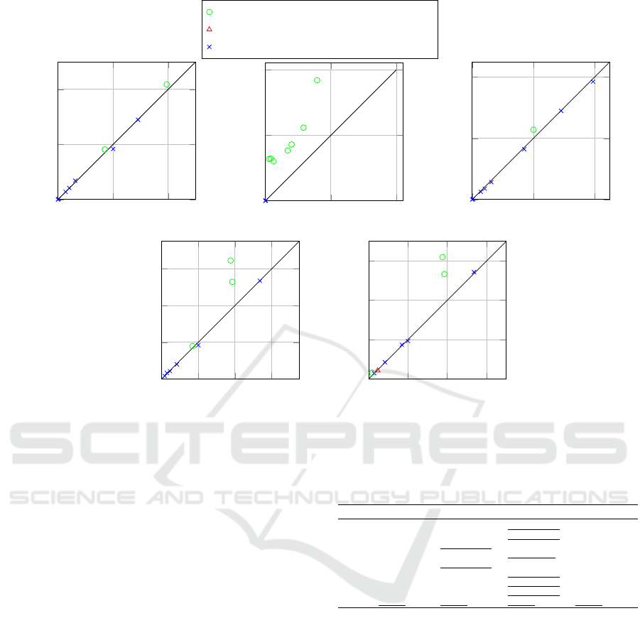
Dataset with Signiﬁcant Deterioration

Dataset with Neither

0 0.02 0.04

0.02

0.04

PTE-ALL

ToP-ALL

0.05

0.1

0.15

0.05

0.1

0.15

PTE-ALL

AdaBoost

0 0.02 0.04

0.02

0.04

PTE-ALL

0.05

0.1

0.15

0.2

0.05

0.1

0.15

0.2

PTE-LR

ToP-LR

0.05

0.1

0.15

0.2

0.05

0.1

0.15

0.2

PTE-LR

Figure 4: Scatter plots contrasting the AUC-Loss of PTE-ALL with baselines ToP-ALL, Random Forest, and AdaBoost, as

well as the AUC-Loss of PTE-LR compared to ToP-LR and Logistic Regression. Each data point in these plots represents the

mean loss obtained over the ten cross-validation folds for a speciﬁc OpenML task. Data points are color-coded to highlight

the statistical signiﬁcance of the performance difference between PTE and the respective baselines.

Table 4: Loss of PTE-ALL and baselines optimised for

ROC-AUC.

Task ID PTE-ALL ToP-ALL RF AdaBoost

14 0.0165±0.003 0.0174±0.0039 0.0166±0.0032 0.0728±0.0184 •

16 0.0019±0.0009 0.0022±0.0012 0.0019±0.0012 0.0489±0.0118 •

18 0.0387±0.0073 0.0377±0.0082 0.0372±0.0072 ◦ 0.1272±0.02 •

20 0.0015±0.0011 0.0015±0.001 0.0011±0.0008 0.0325±0.0105 •

22 0.0209±0.003 0.0207±0.0042 0.0242±0.0036 • 0.0863±0.0397 •

9942 0.0±0.0 0.0±0.0 0.0±0.0 0.0013±0.0042

9955 0.016±0.0033 0.0167±0.0042 0.0145±0.0025 ◦ 0.0787±0.0112 •

9964 0.0038±0.0015 0.0039±0.0017 0.0032±0.001 0.0586±0.0166 •

9979 0.0±0.0 0.0±0.0 0.0±0.0 0.0±0.0

Logistic Regression in three instances, we note that

Logistic Regression slightly surpasses PTE-LR on

ﬁve datasets. A similar pattern of degraded perfor-

mance is observed when comparing ToP-LR to Logis-

tic Regression. These observations suggest that both

tree-based ensemble methods might be overﬁtting the

training data, thereby offering an avenue for further

investigation and optimisation of these methods.

In Table 4, we present the outcomes derived from

PTE-ALL, ToP-ALL, Random Forest, and AdaBoost.

Exploiting a broader set of base learners, we note

outcomes akin to those observed when using solely

Logistic Regression. Speciﬁcally, PTE-ALL out-

performs ToP-ALL in ﬁve scenarios, while the re-

verse occurs in two instances, with no statistically

signiﬁcant differences in these comparisons. How-

ever, PTE-ALL exceeds the performance of Random

Forest in three cases and falls behind in four, with

one instance of statistically signiﬁcant improvement

and two cases of statistically signiﬁcant degradation.

Meanwhile PTE-ALL consistantly outperforms Ad-

aBoost. Taking into account these results, we can

assert that for the AUC-Loss function, incorporating

Class Dichotomies into tree-based ensembling is in-

deed advantageous. Nevertheless, the comparison to

Random Forest raises doubts about the merits of at-

tempting to enhance Random Forest by employing it

as a base learner in PTEs or ToPs.

Evaluating the performance of the three distinct

base learners, we ﬁnd that Random Forest is the

most proﬁcient in capturing the underlying distribu-

tion of the datasets we explored. Given that its base

learners—Decision Trees—have an intrinsic ability

to partition the feature space, we hypothesise that

they might not obtain signiﬁcant advantages from the

tree-based partitioning characteristic of our ensemble

methods.

ICPRAM 2025 - 14th International Conference on Pattern Recognition Applications and Methods

Table 5: Runtime of PTE-ALL and baselines optimised for ROC-AUC.

Task ID PTE-ALL ToP-ALL PTE-LR ToP-LR RF AdaBoost LR

14 171.6819±58.8443 77.7228±19.3721 ◦ 1.0283±0.0362 ◦ 0.5091±0.0336 ◦ 31.272±6.8324 ◦ 3.5745±0.2582 ◦ 0.1625±0.0078 ◦

16 176.6548±72.4138 59.2395±24.3352 ◦ 1.1891±0.6958 ◦ 0.4631±0.0257 ◦ 27.6619±11.8803 ◦ 2.951±0.2188 ◦ 0.1332±0.0067

◦

18 55.1±44.2909 31.1692±20.3078 2.351±0.6888 ◦ 0.3143±0.0415 ◦ 2.0931±1.7565 ◦ 0.1606±0.1092 ◦ 0.1049±0.0019 ◦

20 147.4708±61.4661 60.185±15.4995 ◦ 19.8405±10.0204 ◦ 12.1076±1.5598 ◦ 3.2289±1.1929 ◦ 9.7781±1.0633 ◦ 0.7686±0.4613 ◦

22 89.3503±18.7013 42.5977±6.5014 ◦ 0.9597±0.2382 ◦ 0.4143±0.0595 ◦ 25.8293±2.9524 ◦ 2.3192±0.1968 ◦ 0.1253±0.0027 ◦

9942 771.8217±519.4681 688.7455±305.1365 15.7081±3.163 ◦ 14.4876±2.9639 ◦ 0.7687±1.1615 ◦ 0.6253±0.04 ◦ 0.119±0.0068 ◦

9955 171.4221±47.3616 69.4383±9.6315 ◦ 31.0588±11.3884 ◦ 10.0724±0.5299 ◦ 22.2991±25.0351 ◦ 3.4312±0.7699 ◦ 0.5485±0.0541 ◦

9964 98.5397±45.7543 38.8915±7.974 ◦ 2.0098±0.628 ◦ 0.6526±0.0767 ◦ 2.4775±0.5695 ◦ 1.2225±0.0923 ◦ 0.2283±0.0333 ◦

9979 31.1584±2.2996 15.5143±0.26 ◦ 4.0713±0.6113 ◦ 0.4265±0.0843 ◦ 0.5081±0.7243 ◦ 0.5961±0.0134 ◦ 0.126±0.005 ◦

Table 5 displays the average runtime of each

method and dataset. We observe that PTEs exhibit

signiﬁcantly longer runtimes compared to ToPs for

both families of base learners. The increased runtime

can range from two-fold to almost ten-fold in some

cases.

5.2 Experiments Using F1-Loss

This section outlines the results from our experiments

using the F1-Loss. F1 is a metric that reﬂects a clas-

siﬁer’s precision and recall, thereby providing a bal-

anced evaluation of the model’s performance.

5.2.1 Motivation

The F1-Measure is a widely-used evaluation metric,

due to its ability to better manage class imbalances

compared to accuracy. In situations where the dataset

is unbalanced accuracy tends to become an unreliable

measure because it often gives an overly optimistic es-

timation based on the classiﬁer’s performance on the

majority class, thereby obscuring its potential short-

comings in predicting minority classes (Chicco and

Jurman, 2020). Conversely, the F1-Measure repre-

sents the harmonic mean of Precision and Recall.

Given that the harmonic mean of two numbers tends

to be closer to the smaller one, a high F1-Measure

signiﬁes a strong Recall and Precision, thus providing

a more appropriate measure of the classiﬁer’s perfor-

mance in the presence of class imbalances (Gu et al.,

2009).

5.2.2 Multi-Class F1

In our multi-class classiﬁcation experiments we use

the Macro F1-Score described in (Grandini et al.,

2020). The Macro F1-Score is calculated based on the

Macro Average Precision (MVP) and Recall (MVR).

We calculate the macro average of a measure by ap-

plying it to all classes individually and taking the

arithmetic mean of the results.

Table 6: Loss of PTE-LR and baselines optimised for F1-

Score.

Task ID PTE-LR ToP-LR LR

14 0.1687±0.0302 0.1788±0.0301 • 0.1739±0.0232

16 0.0457±0.0176 0.0425±0.0145 0.0421±0.0162 ◦

18 0.3851±0.1047 0.5287±0.0391 • 0.533±0.032 •

20 0.0285±0.0111 0.0325±0.012 0.029±0.0113

22 0.2003±0.0148 0.1837±0.0366 0.1928±0.0183

9942 0.0174±0.0143 0.0158±0.007 0.0312±0.009 •

9955 0.5356±0.0337 0.5344±0.0314 0.5433±0.0332

9964 0.083±0.0192 0.079±0.0167 0.085±0.0244

9979 0.3761±0.0839 0.645±0.038 • 0.6192±0.0414 •

5.2.3 Experimental Results

In Table 6, we present the mean loss obtained for each

dataset using PTE-LR, ToP-LR, and individual Lo-

gistic Regression when optimising for multi-class F1-

Loss.

Figure 5 provides a visual representation of the re-

sults obtained.

We observe that PTE-LR outperforms ToP-LR in

four cases, with three of them showing statistically

signiﬁcant differences. Conversely, ToP-LR achieves

better results in ﬁve instances, although none of these

differences are statistically signiﬁcant. This pattern,

characterised by slight performance degradation on

some datasets and signiﬁcant gains on others, mirrors

what we previously observed in our experiments with

AUC-Loss.

In Section 5.1.3 we hypothesised that these vari-

ations in performance can be attributed to certain

datasets possessing intrinsic characteristics that make

them more amenable to the application of Class Di-

chotomies. Interestingly, all three datasets that exhib-

ited signiﬁcant improvements in F1-Loss also showed

signiﬁcant improvements in AUC-Loss, reinforcing

our conjecture that, regardless of the loss function em-

ployed, there exists a property in the underlying dis-

tribution that can be more effectively captured when

utilising Class Dichotomies.

On the other hand, the minor performance degra-

dations observed on datasets where this property is

not apparent may again be attributed to factors such

as noise and overﬁtting, which can pose challenges

for the PTEs.

Partition Tree Ensembles for Improving Multi-Class Classiﬁcation

Dataset with Signiﬁcant Improvement

Dataset with Signiﬁcant Deterioration

Dataset with Neither

0 0.2 0.4

0.2

0.4

PTE-ALL

ToP-ALL

0.5

PTE-ALL

AdaBoost

0 0.2 0.4

0.2

0.4

PTE-ALL

0 0.2 0.4

0.6

0.2

0.4

0.6

PTE-LR

ToP-LR

0 0.2 0.4

0.6

0.2

0.4

0.6

PTE-LR

Figure 5: Scatter plots contrasting the F1-Loss of PTE-ALL with baselines ToP-ALL, Random Forest, and AdaBoost, as well

as the F1-Loss of PTE-LR compared to ToP-LR and Logistic Regression.

When comparing PTE-LR with simple Logistic

Regression, we continue to observe a similar pattern

as in the previous experiments. PTE-LR outperforms

Logistic Regression in seven cases, with three of them

showing statistically signiﬁcant improvements. Con-

versely, Logistic Regression outperforms PTE-LR in

two cases, with one of them being statistically signif-

icant. Based on the observed results, it is evident that

overﬁtting is a signiﬁcant challenge for both ToP-LR

and PTE-LR, with the more ﬂexible PTE-LR model

being particularly susceptible. This conclusion is sup-

ported by the fact that, in datasets where individual

Logistic Regression outperforms PTE-LR, ToP-LR

also demonstrates performance superior to PTE-LR.

Therefore, in future research it will be essential to ad-

dress the issue of overﬁtting in order to enhance the

performance of our ensemble method further.

The outcomes of PTE-ALL, ToP-ALL, Random

Forest, and AdaBoost optimised for F1-Loss are pre-

sented in Table 7.

Consistent with previous ﬁndings, PTE-ALL out-

performs ToP-ALL in the majority of cases, with two

instances demonstrating statistical signiﬁcance. Fur-

thermore, there is one case where PTE-ALL exhibits a

signiﬁcant improvement over Random Forest. We ob-

serve that the runtime for optimising F1-Loss is com-

Table 7: Loss of PTE-ALL and baselines optimised for F1-

Score.

Task ID PTE-ALL ToP-ALL RF AdaBoost

14 0.1701±0.0209 0.1818±0.0246 • 0.1644±0.0235 0.3836±0.0634 •

16 0.0411±0.0152 0.0421±0.0114 0.0355±0.0137 0.321±0.1003 •

18 0.2909±0.0233 0.2896±0.0283 0.2899±0.0291 0.5574±0.0789 •

20 0.0279±0.0101 0.028±0.0088 0.0255±0.005 0.318±0.2167 •

22 0.2003±0.0148 0.1837±0.0366 0.2281±0.0291 • 0.4291±0.0626 •

9942 0.0023±0.0074 0.0023±0.0072 0.0014±0.0043 0.0023±0.0074

9955 0.3949±0.049 0.4181±0.0438 • 0.3852±0.0412 0.9187±0.0181 •

9964 0.0624±0.0132 0.0685±0.0114 0.0569±0.0097 0.3017±0.0583 •

9979 0.0±0.0 0.0±0.0 0.0±0.0 0.0±0.0

parable to that of AUC-Loss.

6 CONCLUSION

This paper introduced Partition Tree Ensembles, a

tree-based ensemble method that incorporates ideas

from Nested Dichotomies and Trees of Predictors

to improve multi-class classiﬁcation performance.

Through an extensive experimental evaluation, we

demonstrated that our approach achieves signiﬁcant

performance gains over its predecessor Tree of Pre-

dictors across various datasets and loss functions.

Furthermore, we observed signiﬁcant improvements

over Random Forest on several datasets. In compari-

son with AdaBoost, our method demonstrated signif-

ICPRAM 2025 - 14th International Conference on Pattern Recognition Applications and Methods

icantly higher performance in nearly all cases. How-

ever, this comes at the cost of a signiﬁcantly increased

runtime.

There are several avenues for future research that

stand to be explored. Firstly, we intend to apply PTEs

to other families of base learners. Recent studies

have shown that well-tuned neural networks exhibit

state-of-the-art performance on tabular data (Kadra

et al., 2021), and it would be interesting to investigate

whether ensembling using our Partition Tree Method

can further improve their performance.

Secondly, we suspect that there is potential for en-

hancing performance by employing alternative strate-

gies for selecting and weighting the base learners.

In the current algorithm, the subtrees of each class

dichotomy allocate a portion of the training data

to replace the second validation set. Future work

could explore using greedy forward selection, pro-

posed in (Caruana et al., 2004), to determine the opti-

mal weight for each base learner and the best possible

split using only a single validation set. Furthermore,

it might be valuable to investigate the beneﬁts of re-

taining base learners in the ﬁnal ensemble that were

trained but not selected as optimal.

Finally, an interesting avenue for future research

would be to explore the strategy of sampling a subset

of attributes to evaluate for each split in the tree con-

struction process. This approach has the potential to

mitigate overﬁtting and improve runtime efﬁciency.

In conclusion, the development of Partition Tree

Ensembles presents a promising approach for enhanc-

ing multi-class classiﬁcation performance. By lever-

aging ideas from Nested Dichotomies and Trees of

Predictors, our method offers signiﬁcant performance

gains over the Trees of Predictors method.

ACKNOWLEDGMENTS

This work was performed using resources provided

by the Cambridge Service for Data Driven Discov-

ery (CSD3) operated by the University of Cambridge

Research Computing Service (www.csd3.cam.ac.uk),

provided by Dell EMC and Intel using Tier-2 funding

from the Engineering and Physical Sciences Research

Council (capital grant EP/T022159/1), and DiRAC

funding from the Science and Technology Facilities

Council (www.dirac.ac.uk). For the purpose of open

access, the author has applied a Creative Commons

Attribution (CC BY) licence to any Author Accepted

Manuscript version arising from this submission.

REFERENCES

Beneke, M., K

onig, M., and Link, M. (2023). The inverted

pendulum as a classical analog of the eft paradigm.

Beygelzimer, A., Langford, J., and Ravikumar, P.

(2007). Multiclass classiﬁcation with ﬁlter

trees, 2007. Preprint, available at http://hunch.

net/jl/projects/reductions/mc to b/invertedTree. pdf.

Breiman, L. (2001). Random forests. Machine Learning,

45(1):5–32.

Breiman, L., Friedman, J., Stone, C., and Olshen, R. (1984).

Classiﬁcation and Regression Trees. Taylor & Francis.

Caruana, R., Niculescu-Mizil, A., Crew, G., and Ksikes, A.

(2004). Ensemble selection from libraries of models.

In Proceedings of the Twenty-First International Con-

ference on Machine Learning, ICML ’04, page 18,

New York, NY, USA. Association for Computing Ma-

chinery.

Chicco, D. and Jurman, G. (2020). The advantages of the

matthews correlation coefﬁcient (MCC) over F1 score

and accuracy in binary classiﬁcation evaluation. BMC

Genomics, 21(1):6.

Cortes, C. and Mohri, M. (2003). Auc optimization vs.

error rate minimization. In Thrun, S., Saul, L., and

Sch

olkopf, B., editors, Advances in Neural Informa-

tion Processing Systems, volume 16. MIT Press.

Dua, D. and Graff, C. (2017). UCI machine learning repos-

itory.

Fox, J. (2016). Applied Regression Analysis and General-

ized Linear Models. SAGE, London.

Frank, E. and Kramer, S. (2004). Ensembles of nested di-

chotomies for multi-class problems. In Brodley, C. E.,

editor, Machine Learning, Proceedings of the Twenty-

ﬁrst International Conference (ICML 2004), Banff, Al-

berta, Canada, July 4-8, 2004, volume 69 of ACM In-

ternational Conference Proceeding Series. ACM.

Freund, Y., Schapire, R., and Abe, N. (1999). A short in-

troduction to boosting. Journal-Japanese Society For

Artiﬁcial Intelligence, 14(771-780):1612.

Grandini, M., Bagli, E., and Visani, G. (2020). Metrics for

multi-class classiﬁcation: an overview. arXiv preprint

arXiv:2008.05756.

Gu, Q., Zhu, L., and Cai, Z. (2009). Evaluation measures

of the classiﬁcation performance of imbalanced data

sets. In Cai, Z., Li, Z., Kang, Z., and Liu, Y., editors,

Computational Intelligence and Intelligent Systems,

pages 461–471, Berlin, Heidelberg. Springer Berlin

Heidelberg.

Hand, D. J. and Till, R. J. (2001). A simple generalisation of

the area under the roc curve for multiple class classiﬁ-

cation problems. Machine Learning, 45(2):171–186.

Kadra, A., Lindauer, M., Hutter, F., and Grabocka, J.

(2021). Well-tuned simple nets excel on tabular

datasets. Advances in neural information processing

systems, 34:23928–23941.

Leathart, T., Pfahringer, B., and Frank, E. (2016). Build-

ing ensembles of adaptive nested dichotomies with

random-pair selection. In Frasconi, P., Landwehr,

N., Manco, G., and Vreeken, J., editors, Machine

Learning and Knowledge Discovery in Databases -

Partition Tree Ensembles for Improving Multi-Class Classiﬁcation

European Conference, ECML PKDD 2016, Riva del

Garda, Italy, September 19-23, 2016, Proceedings,

Part II, volume 9852 of Lecture Notes in Computer

Science, pages 179–194. Springer.

Leathart, T. M. (2019). Tree-structured multiclass probabil-

ity estimators. PhD thesis, The University of Waikato,

Hamilton, New Zealand. Doctoral.

Lindauer, M., Eggensperger, K., Feurer, M., Biedenkapp,

A., Deng, D., Benjamins, C., Ruhkopf, T., Sass, R.,

and Hutter, F. (2022). Smac3: A versatile bayesian op-

timization package for hyperparameter optimization.

Journal of Machine Learning Research, 23(54):1–9.

Malerba, D., Appice, A., Bellino, A., Ceci, M., and Pal-

lotta, D. (2001). Stepwise induction of model trees.

In Esposito, F., editor, AI*IA 2001: Advances in Ar-

tiﬁcial Intelligence, pages 20–32, Berlin, Heidelberg.

Springer Berlin Heidelberg.

Maso, G., Businelli, C., Piccoli, M., Montico, M., De Seta,

F., Sartore, A., and Alberico, S. (2012). The clini-

cal interpretation and signiﬁcance of electronic fetal

heart rate patterns 2 h before delivery: an institutional

observational study. Archives of Gynecology and Ob-

stetrics, 286(5):1153–1159.

Mohr, F., Wever, M., and H

ullermeier, E. (2018). Reduction

stumps for multi-class classiﬁcation. In Duivesteijn,

W., Siebes, A., and Ukkonen, A., editors, Advances in

Intelligent Data Analysis XVII, pages 225–237, Cham.

Springer International Publishing.

Pedregosa, F., Varoquaux, G., Gramfort, A., Michel, V.,

Thirion, B., Grisel, O., Blondel, M., Prettenhofer,

P., Weiss, R., Dubourg, V., Vanderplas, J., Passos,

A., Cournapeau, D., Brucher, M., Perrot, M., and

Duchesnay, E. (2011). Scikit-learn: Machine learning

in Python. Journal of Machine Learning Research,

12:2825–2830.

Quinlan, J. R. (1986). Induction of decision trees. Machine

Learning, 1(1):81–106.

Quinlan, J. R. et al. (1992). Learning with continuous

classes. In 5th Australian joint conference on artiﬁ-

cial intelligence, volume 92, pages 343–348. World

Scientiﬁc.

Rey, D. and Neuh

auser, M. (2011). Wilcoxon-Signed-Rank

Test, pages 1658–1659. Springer Berlin Heidelberg,

Berlin, Heidelberg.

Singh, J. (2023). Computational complexity and analysis of

supervised machine learning algorithms. In Kumar,

R., Pattnaik, P. K., and R. S. Tavares, J. M., editors,

Next Generation of Internet of Things, pages 195–206,

Singapore. Springer Nature Singapore.

Torgo, L. (1997a). Functional models for regression tree

leaves. In ICML, volume 97, pages 385–393. Citeseer.

Torgo, L. (1997b). Kernel regression trees. In Poster papers

of the 9th European conference on machine learning

(ECML 97), pages 118–127. Prague, Czech Republic.

Wang, Y. and Witten, I. (1997). Induction of model trees

for predicting continuous classes. Induction of Model

Trees for Predicting Continuous Classes.

Wever, M., Mohr, F., and H

ullermeier, E. (2018). Ensem-

bles of evolved nested dichotomies for classiﬁcation.

In Aguirre, H. E. and Takadama, K., editors, Pro-

ceedings of the Genetic and Evolutionary Computa-

tion Conference, GECCO 2018, Kyoto, Japan, July

15-19, 2018, pages 561–568. ACM.

Wever, M.,

Ozdogan, M., and H

ullermeier, E. (2023). Co-

operative co-evolution for ensembles of nested di-

chotomies for multi-class classiﬁcation. In Proceed-

ings of the Genetic and Evolutionary Computation

Conference, pages 597–605.

Wolpert, D. H. (1992). Stacked generalization. Neural Net-

works, 5(2):241–259.

Yoon, J., Zame, W. R., Banerjee, A., Cadeiras, M., Alaa,

A. M., and van der Schaar, M. (2018a). Personal-

ized survival predictions via trees of predictors: An

application to cardiac transplantation. PLOS ONE,

13(3):e0194985.

Yoon, J., Zame, W. R., and van der Schaar, M. (2018b).

ToPs: Ensemble learning with trees of predictors.

IEEE Transactions on Signal Processing, 66(8):2141–

2152.

APPENDIX

Hyperparameter Tuning

In this Appendix, we outline the hyperparameter tun-

ing procedure employed to optimise our predictors. It

is important to note that we perform hyperparameter

tuning for each cross-validation split and loss function

evaluated.

We implement our hyperparameter tuning proce-

dure using the state-of-the-art Bayesian Optimisation

framework SMAC3 (Lindauer et al., 2022). We em-

ploy the Hyperparameter Tuning facade, which uses

Random Forest as a surrogate model.

However, due to their substantial runtime, con-

ducting a comprehensive hyperparameter tuning pro-

cedure is not feasible within our constraints for both

PTEs and ToPs. Instead, we focus on tuning the hy-

perparameters of their respective base learners on the

speciﬁc dataset at hand. Although the optimal base

learner parameters for standalone use may differ from

those for ensemble methods, we assume that they are

a reasonable approximation.

Furthermore, we choose min leaf samples =

100, slightly higher than (Torgo, 1997a) to mitigate

overﬁtting. As done in (Yoon et al., 2018b), we set

val1 size = 0.15 and val2 size = 0.1.

In Table 8 we present the search space we set

for hyperparameter optimisation. For hyperparame-

ters not mentioned in this table, we rely on the default

values as provided by the scikit-learn library.

ICPRAM 2025 - 14th International Conference on Pattern Recognition Applications and Methods

Table 8: Hyperparameter search spaces.

Classiﬁer Hyperparameter Search Space

Random Forest

n estimators {i|i ∈ N ∧ 10 ≤ i ≤ 1000}

criterion {“gini

′′

,“log loss

′′

}

max depth {i|i ∈ N ∧ 3 ≤ i ≤ 10}

AdaBoost

n estimators {i|i ∈ N ∧ 25 ≤ i ≤ 200}

learning rate [0.5,2.0]

Logistic Regression

penalty {“l2

′′

,“none

′′

}

C [0.5,5.0]

Proof of the Computational Complexity

Proof of Computational Complexity for One

Recursive Step

Statement: For a single recursive step of our

method the computational complexity is given by

∑

i=1

(n,d))

∑

j=1

(n,d) +

∑

i=1

(n,d))

(5)

Proof. Each recursive step consists of two main

parts. First, we create candidate splits of the feature

space as in ToPs. Second, we create candidate Class

Dichotomies.

The computational complexity of the splitting of

the feature space is shown in (Yoon et al., 2018b) to

∑

i=1

(n,d)

. (6)

When creating a candidate Class Dichotomy for an

algorithm A

∈ A

, we use the Random Pair method

to obtain the two meta-classes. In this process, we

require one execution of A

to obtain h

−

, which

is used to determine the meta-classes. Subsequently,

another execution of A

is required to obtain the meta-

classiﬁer h

−

. Additionally, we need to select the

classiﬁers h

−

and h

. Both of these require one

execution each of every algorithm A ∈ A. In total, we

arrive at a complexity of

2 · T

(n,d) +2 ·

∑

i=1

(n,d))

= O

(n,d) +

∑

i=1

(n,d))

(7)

for the creation of a single Class Dichotomy. Since we

repeat this procedure for every A

∈ A

we obtain

the complexity

∑

j=1

(n,d) +

∑

i=1

(n,d))

. (8)

Adding the complexity O(nd

∑

i=1

(n,d))) of split-

ting the feature space we obtain

∑

i=1

(n,d))

∑

j=1



(n,d) +

∑

i=1

(n,d))



. (9)

Proof of Computational Complexity for an Entire

Partition Tree Ensemble

Statement: For constructing an entire Partition

Tree Ensemble the computational complexity is

given by



∑

i=1

(n,d))

∑

j=1



(n,d) +

∑

i=1

(n,d))





. (10)

Proof. To prove this, we must consider the max-

imum number of possible recursions. We know that

there cannot be more recursive calls than the number

of nodes in the tree. Furthermore, we understand that

every leaf node of our Partition Tree contains at least

one sample. Since there are n samples in total, the

tree can have at most n leaves. In Partition Trees, a

node only has children if we split it, in which case it

has two children. Therefore, Partition Trees are full

binary trees. Consequently, the number of recursive

calls is at most 2n − 1. This leads us to the overall

computational complexity of



2n − 1



∑

i=1

(n,d) +

∑

j=1



(n,d)

∑

i=1

(n,d)





= O



∑

i=1

(n,d) +

∑

j=1



(n,d)

∑

i=1

(n,d)





. (11)

Partition Tree Ensembles for Improving Multi-Class Classiﬁcation