Anomalous Water Dataset Captured by Hyperspectral Cameras

Youta Noboru

and Yuko Ozasa

Tokyo Denki University, 5 Senju Asahi-cho, Adachi-ku, Tokyo, Japan

Keywords:

Hyperspectral Image, Dataset, Water, Anomaly Detection.

Abstract:

This paper proposes a hyperspectral dataset designed for detecting anomalies in water caused by the mixing of

colorless and transparent anomalous liquids. Detecting such anomalous substances, particularly when they are

transparent, is crucial for public health and environmental safety, as conventional methods often inadequate.

Hyperspectral imaging captures subtle spectral differences, enabling the identiﬁcation of materials that are

visually indistinguishable. The dataset aims to support the development of unsupervised learning models that

can detect anomalous substances in water using only a spectral data. We have made this dataset publicly

available (https://github.com/033labcodes/visapp25\ Anomalous-Water-Dataset) to facilitate further research

in this area.

1 INTRODUCTION

It is unacceptable to mix toxins into the drinking wa-

ter or food of animals, but many animals lose their

lives due to this abuse. If the anomalous water ap-

pears the same as usual, colorless and transparent, the

animals may drink it without hesitation. To protect

these animals from such cruelty, it is essential to de-

velop a method that can determine the safety of their

drinking water.

Our task is to detect the colorless and transparent

substances that are indistinguishable in water using

cameras. If the anomalous substances are not col-

orless and transparent, they could be visually iden-

tiﬁable. Therefore, we aim to tackle a case when

the anomalous substances are colorless and transpar-

ent. There are surveillance cameras in areas where

animals are kept, so being able to detect anomalies

through image analysis could help protect the ani-

mals.

We apply Hyperspectral (HS) cameras to our task

since the cameras are effective in detecting differ-

ences that are imperceptible to the human eye. (Su

et al., 2021). Related work on HS imagery analy-

sis, especially on anomaly detection, has primarily

focused on water-related phenomena. These stud-

ies typically target issues such as algal blooms or oil

spills in rivers and lakes, often utilizing drone or satel-

lite imagery (Du et al., 2021). These applications dif-

https://orcid.org/0009-0003-0123-9822

https://orcid.org/0000-0001-9450-0708

fer signiﬁcantly from our work in both purpose and

setting. Most work based on HS image analyzes and

classiﬁes data based on the spectral information of in-

dividual pixels (Su et al., 2021). Therefore, we also

employ pixel-wise HS data to our task, the detection

of anomalous substances dissolved in water that are

colorless and transparent.

Our task should be achieved through unsupervised

learning. The types of anomalous substances present

in the water and their proportions are unknown. So,

it is challenging to gather training data for anomalous

conditions in advance. Since no work has addressed

the same task setting as ours, we ﬁrst validate the ef-

fectiveness of using HS data for our task by employ-

ing commonly used unsupervised anomaly detection

methods for HS data.

In this paper, we propose a dataset to evaluate the

effectiveness of HS data for our task. Our dataset con-

sists of images captured by a HS camera, containing

both normal water and water mixed with anomalous

substances which are colorless and transparent. We

analyze the characteristics of HS data in our task us-

ing the dataset and further evaluate it through unsu-

pervised anomaly detection.

We analyze the characteristics of the proposed

dataset by comparing the spectral signatures of nor-

mal water with those contaminated by various sub-

stances. Our analysis reveals subtle spectral differ-

ences, particularly in non-visible regions, that are un-

detectable to the human eyes or standard RGB cam-

eras. Based on these results, HS data which includes

442

Noboru, Y. and Ozasa, Y.

Anomalous Water Dataset Captured by Hyperspectral Cameras.

DOI: 10.5220/0013163800003912

Paper published under CC license (CC BY-NC-ND 4.0)

In Proceedings of the 20th International Joint Conference on Computer Vision, Imaging and Computer Graphics Theory and Applications (VISIGRAPP 2025) - Volume 3: VISAPP, pages

442-449

ISBN: 978-989-758-728-3; ISSN: 2184-4321

(a) Normal water. (b) Water mixed with detergent.

Figure 1: RGB samples of normal water and water mixed with anomalous substances.

not only visible but also non-visible spectral informa-

tion, has the potential to be effective for our task.

We compare the performance of various unsuper-

vised anomaly detection methods using both RGB

and HS imaging in our experimental evaluation.

Our results demonstrate the clear superiority of HS

imaging over conventional RGB imaging, with the

best-performing methods achieving an AUCROC of

0.78 for HS data compared to only 0.62 for RGB

data. Additionally, we investigate the robustness of

these methods to unknown anomalies. While per-

formance decreased in this scenario, several methods

still demonstrated promising detection capabilities.

2 RELATED WORK

HS imaging is known to be effective when the dif-

ferences of the targets are difﬁcult to distinguish with

the human eye, as it captures not only the visible spec-

trum but also the non-visible spectrum with high spec-

tral resolution. For example, it is particularly useful

when the target is far away and only a few pixels can

be captured, or when the human eye cannot differen-

tiate based on color.

Although not directly related to our task, there

is work on HS imaging related to water, such as

work focused on water quality monitoring (Brando

and Dekker, 2003). HS datasets speciﬁcally designed

for water quality are less common but are gaining at-

tention, with some datasets speciﬁcally tailored for

anomaly detection (Cao et al., 2021; VanderWoude

and Marshall, 2021). These datasets focus on detect-

ing subtle spectral changes that may indicate the pres-

ence of pollutants, algae blooms, or chemical contam-

ination in water bodies.

Work on unsupervised anomaly detection using

HS data often focuses on detecting changes in land

cover or buildings. However, there are no task set-

tings similar to the one presented in this paper. For a

ﬁrst step in our work, we construct a HS dataset for

our task and evaluate the dataset using unsupervised

anomaly detection methods that are commonly used

for comparative evaluation in HS data (Zhao et al.,

2019).

3 DATASET

We construct a HS image dataset comprising three

types of anomalous substances. These anomalous

substances are mixed with water, poured into a dish,

and then captured by HS camera. Figure 1 illustrates

the RGB samples derived from the HS images. The

three types of anomalous substances included in the

dataset are herbicide, detergent, and chlorine bleach,

all anomalous substances not meant for consumption.

As evident from the ﬁgure, there are no discernible

Anomalous Water Dataset Captured by Hyperspectral Cameras

443

Figure 2: Scene of dataset capture: HS camera positioned

above dishes containing water samples.

differences visible to the eye.

We capture a total of 80 HS images. For each nor-

mal and anomalous substance, images are taken from

10 different positions. At each position, images are

taken with exposure settings adjusted to both the vis-

ible spectrum and the near-infrared (NIR) spectrum.

We utilize the NH-9 HS Camera by evaJapan (Eba

Japan Co.Ltd., ), which is capable of capturing a

spectral range from 350[nm] to 1100[nm] across 151

bands, with a spatial resolution of 5[nm]. The cam-

era records data in raw format, providing pixel val-

ues ranging from 0 to 4095, allowing for a detailed

spectral analysis. The images have a resolution of

2048 × 1080 pixels.

Figure 2 depicts the setup for capturing the

dataset. The dataset was recorded in a darkroom with

halogen lighting. The camera was positioned directly

above the dish. The distance between the camera and

the dish was 55[cm]. To ensure diversity and pre-

vent the creation of identical samples under the same

imaging conditions, the dish is randomly repositioned

by approximately 5[cm] between each pair of visible

and NIR HS images.

To facilitate the evaluation of methods focusing on

HS image pixels, we annotated the dataset. Each HS

image in the dataset is labeled with binary indicators

denoting whether the sample is normal or anomalous

and specifying the name of the anomalous substance.

Additionally, as shown in Figure 3, mask images were

created to delineate pixel regions extracted from the

HS images.

4 DATA ANALYSIS

4.1 Preprocessing Techniques

To analyze the HS data, we ﬁrst extract HS data

containing spectral information from the HS images,

where HS data is denoted as a pixel value extracted

from HS image. First, we apply black level correction

Figure 3: Example of mask images used for pixel extraction

from HS images.

to remove both the DC offset from the analog circuits

and the dark current noise inherent to the pixel com-

ponents. To further reduce noise, we apply a 9 × 9

smoothing ﬁlter. Then, the HS data are extracted from

the HS images using mask images, with each HS im-

age yielding approximately 490, 000 pixels.

We pre-process the HS data for the analysis

through visualization. For the visualization of the

spectra of HS data, the data is scaled to a range of

0 to 1 by dividing by 4095 since the range of the HS

data is 0 to 4095.

4.2 Spectral Analysis in the Visible and

Near-Infrared Regions

Figures 4 present the mean and standard deviation of

the HS images extracted from normal samples in the

dataset. The normal sample is denoted as the HS data

of the normal water. Figure 4a shows the spectral data

with exposure time optimized for the visible light re-

gion, while Figure 4b displays the data with exposure

time adjusted for the NIR region. Hereafter, we will

refer to these as “visible light data” and “NIR data”

respectively.

The spectral ﬁgures provide insights into our

dataset’s characteristics. Figure 4a shows that the

550[nm] − 750[nm] range is captured with high in-

tensity due to optimized exposure. However, inten-

sity decreases toward the non-visible regions, with

increased data variance below 400[nm] and above

1000[nm], likely due to a lower signal-to-noise ratio

after black level correction.

The NIR data in Figure 4b highlights the effective-

ness of adjusting exposure time for the NIR region.

In contrast to Figure 4a, it shows extended and high-

sensitivity capture in the longer wavelengths. Signals

in the 600[nm] − 750[nm] range are saturated due to

increased exposure, while the data reveals a broad and

well-captured spectral range in the NIR.

We constructed combined Visible+NIR data

through band selection from both datasets. The

VISAPP 2025 - 20th International Conference on Computer Vision Theory and Applications

444

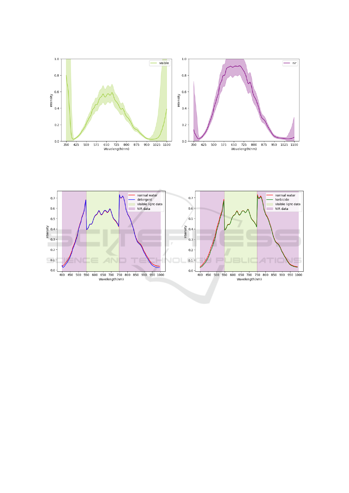
(a) Visible light data. (b) NIR data.

Figure 4: Spectral characteristics of normal water samples. (a) Data optimized for exposure time in the visible light spectrum.

(b) Data optimized for exposure time in the Near-Infrared (NIR) region. In both graphs, the dark line represents the mean

spectral values, while the lighter shaded area indicates the standard deviation.

Figure 5: Comparison of average Visible+NIR spectra be-

tween normal water and water contaminated with detergent.

visible range includes 550[nm] − 750[nm], and the

NIR ranges are 400[nm] − 550[nm] and 750[nm] −

1000[nm]. This approach maximizes sensitivity from

both datasets, with a 5[nm] recording interval, result-

ing in 120 bands spanning 400[nm] − 1000[nm].

4.3 Comparison of Spectral Signatures

Between Normal and Anomalous

Samples

Figures 5 to 7 compare the average Visible+NIR spec-

tra of normal water and three anomalous samples: de-

tergent, herbicide, and chlorine bleach. These plots

span the 400 − 1000[nm] range, constructed through

selective band selection as detailed in Section 4.2.

In Figure 5, the spectrum of detergent-

contaminated water closely resembles normal

Figure 6: Comparison of average Visible+NIR spectra be-

tween normal water and water contaminated with herbicide.

water across most wavelengths. However, subtle

deviations around 400[nm] and 900[nm] are more

noticeable in the NIR region, captured with optimized

exposure settings.

Figure 6 compares the spectra of normal water and

water mixed with herbicide. While largely similar,

subtle differences appear near 400[nm] and 520[nm].

These distinctions are more evident in the NIR region

than in the visible range.

Figure 7 compares chlorine bleach, revealing

more pronounced spectral differences than other sam-

ples. Unlike detergent and herbicide, chlorine bleach

shows signiﬁcant distinctions in the visible range,

highlighting its unique spectral signature.

These analyses demonstrate the value of HS imag-

ing in detecting subtle spectral differences beyond hu-

man visible perception, allowing for effective distinc-

tion between normal and contaminated water.

Anomalous Water Dataset Captured by Hyperspectral Cameras

445

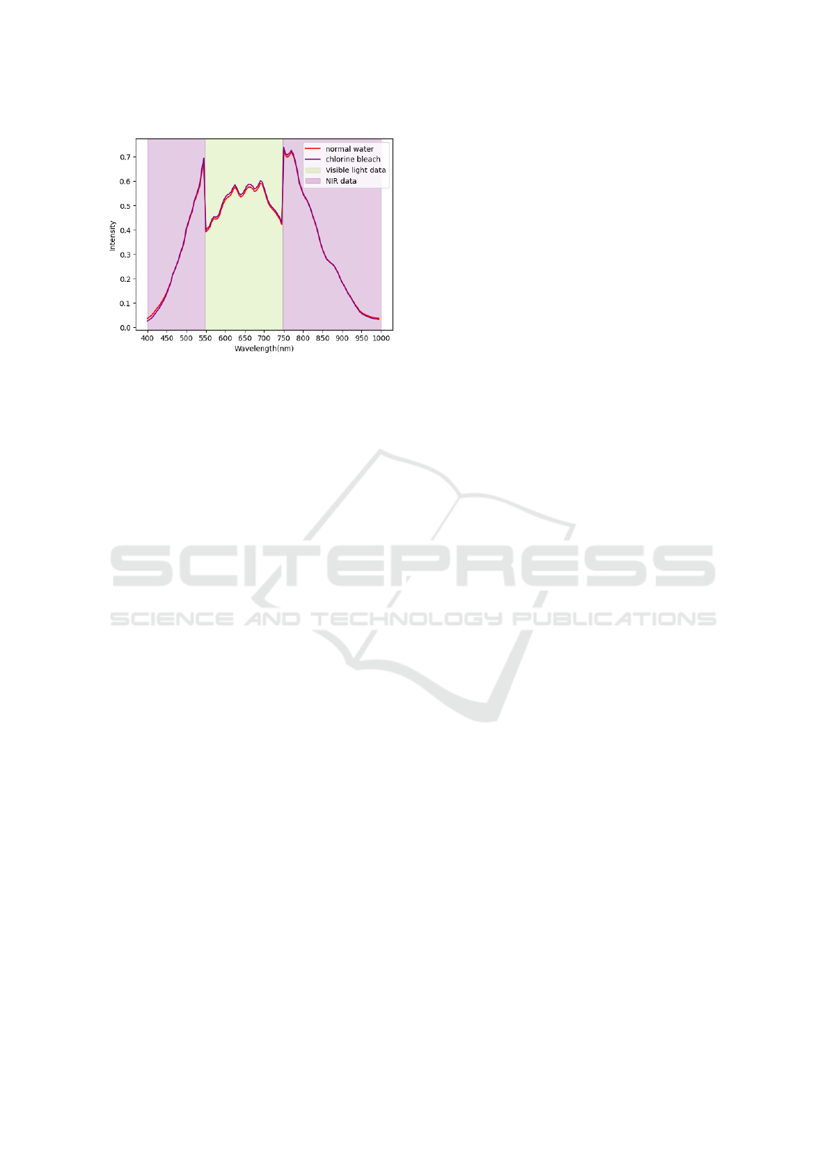
Figure 7: Comparison of average Visible+NIR spectra be-

tween normal water and water contaminated with chlorine

bleach.

5 EVALUATION OF ANOMALY

DETECTION

5.1 Experimental Setup

5.1.1 Dataset and Sampling Methodology

For our experiments, we utilized distinct HS images

for training and evaluation purposes. The HS images,

capturing both normal water and water mixed with

three different types of anomalous substances, were

initially divided into training and evaluation sets at a

7:3 ratio for each substance type. Then, we performed

spectral extraction on these sets using mask images,

followed by conducted band selection. We standard-

ized the extracted HS data by calculating the mean

and standard deviation for each image individually.

Our protocol randomly selected 7, 000 HS data

points from training samples and 3, 000 from evalu-

ation samples, ensuring 10% anomalies evenly dis-

tributed across three types. Each experiment was re-

peated 10 times, and we report the mean results.

5.1.2 Hardware and Software Speciﬁcations

The experiments were conducted on a high-

performance workstation equipped with an Intel i9-

13900k processor operating at 5.8GHz, 128GB of

RAM, and 24 cores. For the implementation of

anomaly detection methods, we employed the Pyod

library (Zhao et al., 2019). The computation of eval-

uation metrics was facilitated by the scikit-learn li-

brary (Pedregosa et al., 2011).

5.1.3 Evaluation Metrics

To assess the efﬁcacy of our experiments on anomaly

detection, we employed two primary metrics: AU-

CROC (Area Under the Receiver Operating Charac-

teristic Curve) and Precision.

The AUCROC metric measures the area under

the ROC curve, representing the relationship between

True Positive Rate (TPR) and False Positive Rate

(FPR) across thresholds. Ranging from 0.5 to 1,

higher values indicate better performance. It is robust

against class imbalance, ensuring reliable evaluations

even with few anomalous samples.

Precision measures the proportion of true anoma-

lies among instances classiﬁed as anomalous. This

metric evaluates the reliability of the model’s positive

anomaly predictions.

5.1.4 Unsupervised Anomaly Detection Method

and Hyperparameters

The unsupervised anomaly detection methods utilized

in our experiments are enumerated below. For each

method, we adhered to the default hyperparameter

values provided by the respective libraries to maintain

consistency and reproducibility in our experimental

setup.

• Isolation Forest (Liu et al., 2008). Isolates obser-

vations by randomly selecting features and split

values to partition the data.

• K Nearest Neighbors (KNN) (Ramaswamy

et al., 2000). KNN views the anomaly score of

the input instance as the distance to its k-th near-

est neighbor.

• Principle Component Analysis (PCA) (Shyu

et al., 2003). PCA is a linear dimensionality re-

duction technique. When used for AD, it projects

the data to a lower dimensional space and uses the

reconstruction errors as anomaly scores.

• One-Class SVM (OCSVM) (Scholkopf et al.,

2001). OCSVM maximizes the margin between

the origin and the normal samples, and deﬁnes

the decision boundary as the hyperplane that de-

termines the margin.

• Subspace Outlier Detection (SOD) (Kriegel

et al., 2009). SOD aims to detect outliers in vary-

ing subspaces of high-dimensional feature space.

• Cluster-based Local Outlier Factor

(CBLOF) (He et al., 2003). CBLOF calcu-

lates the anomaly score by ﬁrst assigning samples

to clusters, and then using the distance among

clusters as anomaly scores.

VISAPP 2025 - 20th International Conference on Computer Vision Theory and Applications

446

Table 1: Comparison of unsupervised anomaly detection performance using visible light data, NIR data, and combined

Visible+NIR data across various detection methods.

Method

Spectral Ranges

Visible light data NIR data Visible + NIR data

AUCROC Precision AUCROC Precision AUCROC Precision

Isolation Forest (Liu et al., 2008) 0.49 0.10 0.50 0.09 0.50 0.10

KNN (Ramaswamy et al., 2000) 0.67 0.44 0.63 0.41 0.64 0.46

PCA (Shyu et al., 2003) 0.49 0.09 0.49 0.08 0.49 0.09

OCSVM (Scholkopf et al., 2001) 0.49 0.09 0.49 0.08 0.49 0.08

SOD (Kriegel et al., 2009) 0.77 0.50 0.76 0.51 0.77 0.52

CBLOF (He et al., 2003) 0.53 0.16 0.51 0.12 0.50 0.10

ABOD (Kriegel et al., 2008) 0.71 0.25 0.75 0.29 0.75 0.23

LOF (Breunig et al., 2000) 0.68 0.27 0.77 0.52 0.78 0.45

COF (Tang et al., 2002) 0.77 0.60 0.78 0.65 0.78 0.70

• Angle-based Outlier Detector (ABOD) (Kriegel

et al., 2008). ABOD measures the variance in an-

gles between a point and pairs of other points.

Lower angle variance indicates a higher likeli-

hood of being an outlier.

• Local Outlier Factor (LOF) (Breunig et al.,

2000). LOF measures the local deviation of the

density of a given sample with respect to its neigh-

bors.

• Connectivity-based Outlier Factor(COF) (Tang

et al., 2002). COF uses the ratio of the average

chaining distance of data points and the average

chaining distance of k-th nearest neighbor of the

data point, as the anomaly score for observations.

5.2 Analysis of Different Spectral

Ranges for Anomaly Detection

Table 1 presents the performance of various anomaly

detection methods across different spectral ranges.

We evaluated the methods using visible light data,

NIR data, and the combined Visible+NIR data con-

structed through our band selection approach. The

highest performance for each metric is highlighted in

bold, with the second-highest underlined.

Our analysis shows that the COF method, applied

to combined Visible+NIR data, achieved the highest

performance with an AUCROC of 0.78 and a Preci-

sion of 0.70. This highlights the value of utilizing

both visible and NIR spectral ranges for effective wa-

ter anomaly detection.

Interestingly, when comparing the performance

between the visible light data and NIR data ranges, we

observed a slight advantage for the NIR data. For in-

stance, COF applied to NIR data yielded an AUCROC

of 0.78 and Precision of 0.65, compared to 0.77 and

0.60 for the visible light data, respectively. This

trend was consistent across several methods, suggest-

ing that the NIR data region is able to capture subtle

Table 2: Comparison of Anomaly Detection Methods.

Method

Data type

RGB HS

AUCROC Precision AUCROC Precision

Isolation Forest 0.50 0.09 0.50 0.10

KNN 0.54 0.17 0.64 0.46

PCA 0.49 0.09 0.49 0.09

OCSVM 0.49 0.09 0.49 0.08

SOD 0.62 0.28 0.77 0.52

CBLOF 0.50 0.11 0.50 0.10

ABOD 0.50 0.00 0.75 0.23

LOF 0.51 0.11 0.78 0.45

COF 0.51 0.11 0.78 0.70

spectral differences that are particularly relevant for

detecting anomalies in water samples.

Across all three types of spectral regions, we

noted similar performance patterns among the tested

methods. Distance-based anomaly detection ap-

proaches such as KNN, LOF and COF, along with

subspace-based methods like SOD, demonstrated par-

ticular efﬁcacy for this task. The angle-based method,

ABOD, also showed promising results. In contrast,

methods such as Isolation Forest, PCA, and OCSVM

exhibited AUCROC values close to 0.5, indicating

poor efﬁcacy for this anomaly detection task.

These ﬁndings underscore the importance of se-

lecting optimal spectral ranges and detection meth-

ods for water anomaly detection. The superior perfor-

mance of combined Visible+NIR data suggests that

HS approaches effectively capture a broader range of

anomalies. Additionally, the success of distance- and

subspace-based methods indicates that anomalies in

our dataset are better deﬁned by local density varia-

tions or speciﬁc feature subspaces than by global dis-

tributions.

Anomalous Water Dataset Captured by Hyperspectral Cameras

447

Table 3: Robustness to Unknown Anomalies: Unsupervised anomaly detection performance when trained on one anomalous

type and evaluated on other anomalous types.

Method

Training sample

detergent herbicide chorine bleach

AUCROC Precision AUCROC Precision AUCROC Precision

Isolation Forest (Liu et al., 2008) 0.50 0.03 0.49 0.09 0.49 0.09

KNN (Ramaswamy et al., 2000) 0.61 0.13 0.67 0.48 0.52 0.20

PCA (Shyu et al., 2003) 0.50 0.03 0.48 0.08 0.49 0.08

OCSVM (Scholkopf et al., 2001) 0.49 0.03 0.48 0.07 0.49 0.08

SOD (Kriegel et al., 2009) 0.81 0.23 0.71 0.45 0.65 0.40

CBLOF (He et al., 2003) 0.52 0.04 0.50 0.11 0.50 0.11

ABOD (Kriegel et al., 2008) 0.68 0.06 0.73 0.20 0.67 0.18

LOF (Breunig et al., 2000) 0.73 0.12 0.79 0.39 0.70 0.35

COF (Tang et al., 2002) 0.79 0.31 0.69 0.56 0.64 0.51

5.3 Comparison of Unsupervised

Anomaly Detection Performance

Between RGB and HS Data

Our experimental results, presented in Table 2,

demonstrate a clear superiority of HS imaging over

conventional RGB imaging for the anomaly detection.

For the HS data, we utilized a combined Visible+NIR

dataset spanning 400-1000 nm with 120 bands, as

detailed in Section 4.2. The table shows the per-

formance of various unsupervised anomaly detection

methods applied to both RGB and HS data, evaluated

using AUCROC and Precision metrics.

For RGB data, the subspace-based method SOD

exhibited the highest performance, achieving an AU-

CROC of 0.62 and Precision of 0.28. However, other

methods applied to RGB data failed to yield signiﬁ-

cant results, with most approaches barely outperform-

ing random guessing.

In signiﬁcant contrast to the RGB data results,

the application of these methods to HS data yielded

substantially improved outcomes. The COF method

demonstrated the best performance, attaining an AU-

CROC of 0.78 and an impressive Precision of 0.70.

Similarly, the SOD method also performed well with

HS data, achieving an AUCROC of 0.77 and Preci-

sion of 0.52.

It is noteworthy that multiple methods, including

COF, showed marked improvements when applied to

HS data compared to their RGB counterparts. This

consistent enhancement across various algorithms un-

derscores the inherent value of HS imaging in this

context.

These results provide compelling evidence that

HS imaging can capture subtle spectral differences

imperceptible to the human eye or standard RGB

cameras. The superior performance of anomaly de-

tection methods on HS data demonstrates its efﬁcacy

in identifying potentially hazardous substances in wa-

ter, even when these substances are visually indistin-

guishable from normal samples.

5.4 Robustness to Unknown Anomalies

The robustness of anomaly detection methods to un-

known contaminants is an important consideration

for potential applications in real-world water qual-

ity monitoring. Table 3 presents our ﬁndings, where

models were trained on one type of anomalous sam-

ples and tested on others. For each training sample,

the best-performing method is highlighted in bold,

and the second-best is underlined.

As anticipated, performance decreased compared

to when all types of anomalous samples were in-

cluded in training. However, several methods still

demonstrated signiﬁcant detection capabilities, par-

ticularly for herbicide and chlorine bleach. The COF

method showed the best overall performance, achiev-

ing an AUCROC of 0.69 and precision of 0.56 for

herbicide, and 0.64 and 0.51 respectively for chlorine

bleach.

Consistent with our previous results, distance-

based methods (KNN, LOF, COF) and the subspace-

based method (SOD) proved most effective across all

anomalous types. The angle-based method (ABOD)

also showed promise, especially for herbicide and

chlorine bleach detection. In contrast, Isolation For-

est, PCA, and OCSVM demonstrated poor efﬁcacy in

this setting.

The observed variations in performance across

different training samples indicate the challenge of

generalizing anomaly detection models to unknown

contaminants. Detergent-trained models showed

lower generalization compared to herbicide or chlo-

rine bleach-trained models, suggesting that some con-

taminants may have more distinctive spectral signa-

tures allowing better generalization.

In conclusion, although detecting unknown con-

VISAPP 2025 - 20th International Conference on Computer Vision Theory and Applications

448

taminants is challenging, our results demonstrate that

carefully selected unsupervised learning methods can

offer meaningful detection capabilities. The robust-

ness of these methods to unknown contaminants is

crucial for the practical implementation of water qual-

ity monitoring systems.

6 CONCLUSION

This paper presented a novel HS dataset for detect-

ing anomalous substances in water that are visually

indistinguishable. Our comprehensive spectral analy-

sis demonstrates the superiority of HS imaging over

conventional RGB imaging in capturing subtle dif-

ferences between normal water and water contami-

nated with anomalous substances. Experimental eval-

uations of various unsupervised anomaly detection

methods shows the effectiveness of distance-based

and subspace-based approaches, particularly when

utilizing combined visible and near-infrared spectral

data.

While challenges remain in detecting unknown

anomalies, our ﬁndings provide a foundation for fu-

ture work. Further work could explore advanced deep

learning techniques for HS data and methods to im-

prove generalization. Expanding the dataset to in-

clude more substances could also enhance this work’s

scope.

ACKNOWLEDGEMENTS

This research was supported by the KDDI Founda-

tion. We are grateful to our laboratory members for

their invaluable assistance in this work. Their meticu-

lous work in data acquisition is crucial to the success

of our work.

REFERENCES

Brando, V. E. and Dekker, A. G. (2003). Satellite hy-

perspectral remote sensing for estimating estuarine

and coastal water quality. IEEE transactions on geo-

science and remote sensing, 41(6):1378–1387.

Breunig, M. M., Kriegel, H.-P., Ng, R. T., and Sander, J.

(2000). Lof: identifying density-based local outliers.

SIGMOD Rec., 29(2):93–104.

Cao, Q., Yu, G., Sun, S., Dou, Y., Li, H., and Qiao, Z.

(2021). Monitoring water quality of the haihe river

based on ground-based hyperspectral remote sensing.

Water, 14(1):22.

Du, Q., Tang, B., Xie, W., and Li, W. (2021). Parallel and

distributed computing for anomaly detection from hy-

perspectral remote sensing imagery. Proceedings of

the IEEE, 109(8):1306–1319.

Eba Japan Co.Ltd. Hyper spetral camera NH9. https:

//ebajapan.jp/products/hyper-spectral-camera/.

He, Z., Xu, X., and Deng, S. (2003). Discovering

cluster-based local outliers. Pattern Recogn. Lett.,

24(9–10):1641–1650.

Kriegel, H.-P., Kr

oger, P., Schubert, E., and Zimek, A.

(2009). Outlier detection in axis-parallel subspaces

of high dimensional data. In Proceedings of the

13th Paciﬁc-Asia Conference on Advances in Knowl-

edge Discovery and Data Mining, PAKDD ’09, page

831–838, Berlin, Heidelberg. Springer-Verlag.

Kriegel, H.-P., Schubert, M., and Zimek, A. (2008). Angle-

based outlier detection in high-dimensional data. In

Knowledge Discovery and Data Mining.

Liu, F. T., Ting, K. M., and Zhou, Z.-H. (2008). Isolation

forest. In 2008 Eighth IEEE International Conference

on Data Mining, pages 413–422.

Pedregosa, F., Varoquaux, G., Gramfort, A., Michel, V.,

Thirion, B., Grisel, O., Blondel, M., Prettenhofer,

P., Weiss, R., Dubourg, V., Vanderplas, J., Passos,

A., Cournapeau, D., Brucher, M., Perrot, M., and

Duchesnay, E. (2011). Scikit-learn: Machine learning

in Python. Journal of Machine Learning Research,

12:2825–2830.

Ramaswamy, S., Rastogi, R., and Shim, K. (2000). Efﬁ-

cient algorithms for mining outliers from large data

sets. SIGMOD Rec., 29(2):427–438.

Scholkopf, B., Platt, J. C., Shawe-Taylor, J., Smola, A., and

Williamson, R. C. (2001). Estimating the support of

a high-dimensional distribution. Neural Computation,

13:1443–1471.

Shyu, M.-L., Chen, S., Sarinnapakorn, K., and Chang, L.

(2003). A novel anomaly detection scheme based on

principal component classiﬁer.

Su, H., Wu, Z., Zhang, H., and Du, Q. (2021). Hyperspec-

tral anomaly detection: A survey. IEEE Geoscience

and Remote Sensing Magazine, 10(1):64–90.

Tang, J., Chen, Z., Fu, A. W.-C., and Cheung, D. W.-L.

(2002). Enhancing effectiveness of outlier detections

for low density patterns. In Paciﬁc-Asia Conference

on Knowledge Discovery and Data Mining.

VanderWoude, A. and Marshall, L. (2021). Hyperspectral

imagery to study harmful algal blooms (habs) of lake

erie, lake st. clair, and saginaw bay, lake huron of the

great lakes region.

Zhao, Y., Nasrullah, Z., and Li, Z. (2019). Pyod: A python

toolbox for scalable outlier detection. Journal of Ma-

chine Learning Research, 20(96):1–7.

Anomalous Water Dataset Captured by Hyperspectral Cameras

449