Combining Procedural Generation and Genetic Algorithms

to Model Urban Growth

Etienne Tack

1,2 a

, Gilles

2 b

and Fr

eric Flouvat

3 c

INSIGHT SAS, Noumea, New Caledonia

University of New Caledonia, ISEA, Noumea, New Caledonia

Aix-Marseille Univ., CNRS, LIS, Marseille, France

ﬂ

Keywords:

Procedural Generation, Genetic Algorithm, Agent-Based Modelling, Urban Growth.

Abstract:

In this paper, we present an approach to model spatial inﬂuences in multi-agent models using procedural

generation and genetic algorithms. We applied this approach in an urban growth model. In agent-based

simulations, the agents make decisions based on the perception of their environment. In our context, the

agents represent inhabitants who can create new buildings or extend the existing ones. Their behaviour is

ruled by spatial inﬂuences (e.g., the proximity of the road increases chances of building in the surrounding

areas). Procedural generation provides a good framework for representing the inﬂuences of the environment

on the agent’s behaviour. Each spatial feature is associated with an inﬂuence function. Their parameters

search space can be tremendous, making it difﬁcult for ﬁeld experts to set them manually. Consequently, we

use a genetic algorithm to optimize the parameters of these inﬂuence functions and train the model based on

three spatial measures (Chamfer distance, kernel density, and a density grid). This approach can be employed

likewise to any problem where the agent decisions are wholly or partly based on location. Our experiments

highlight the interest of our approach and the impact of the chosen ﬁtness functions.

1 INTRODUCTION

Urban growth poses signiﬁcant challenges, partic-

ularly in developing regions where informal settle-

ments often emerge without strict planning rules.

These areas, deﬁned by UN-Habitat as lacking secure

tenure, basic infrastructure, and adherence to build-

ing regulations, are shaped by unspoken traditions

and geographical constraints. Existing urban growth

models, including multi-agent systems, often assume

rigid spatial structures like grid layouts, making them

poorly suited for informal contexts.

Multi-agent systems have been widely used to

simulate urban dynamics by modelling individuals

or households as agents. While grid-based ap-

proaches (Schelling, 1971; Barros, 2004; Zhang et al.,

2010; Jokar Arsanjani et al., 2013; Schwarz et al.,

2016; Picascia and Yorke-Smith, 2017; Agyemang

et al., 2022) simplify implementation, they rely on

strong assumptions, such as ﬁxed spatial resolution

https://orcid.org/0000-0003-4131-1449

https://orcid.org/0000-0002-0140-5291

https://orcid.org/0000-0001-7288-0498

and uniform building characteristics, limiting realism.

More precise vector-based approaches (Augustijn-

Beckers et al., 2011) better reﬂect spatial variation

but often embed restrictive local assumptions about

construction patterns. In computer graphics, proce-

dural generation has also been applied to create vir-

tual cities (Smelik et al., 2014), yet these approaches

rarely validate spatial accuracy beyond visual assess-

ments.

Addressing these gaps, this study proposes a novel

method combining procedural generation and genetic

algorithms to model spatial dynamics in agent-based

urban growth simulations. Inspired by Tobler’s ﬁrst

law of geography (Tobler, 1970), which emphasizes

proximity effects, we deﬁne two types of spatial in-

ﬂuence functions and optimize their parameters using

NSGA-II. Our approach eliminates the need for em-

pirical assumptions and improves realism by learning

from spatial data. Experiments demonstrate the ap-

plicability of this method in generating realistic urban

growth patterns, validated through measures like den-

sity differences and Chamfer distance.

420

Tack, E., Énée, G. and Flouvat, F.

Combining Procedural Generation and Genetic Algorithms to Model Urban Growth.

DOI: 10.5220/0013165200003890

Paper published under CC license (CC BY-NC-ND 4.0)

In Proceedings of the 17th International Conference on Agents and Artiﬁcial Intelligence (ICAART 2025) - Volume 1, pages 420-428

ISBN: 978-989-758-737-5; ISSN: 2184-433X

2 THE INFLUENCE SUB-MODEL

Usually, agents are inﬂuenced by their local percep-

tion of the world. In our work, we use inﬂuence func-

tions to determine where agents may construct new

buildings at each iteration of the simulation. An in-

ﬂuence function is deﬁned, with the help of an expert

(geographer), for each environmental factor that is re-

lated to construction of new buildings.

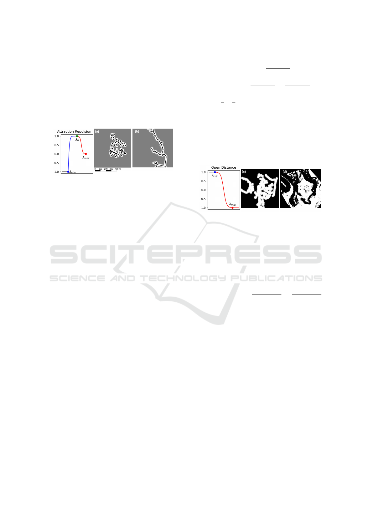
Figure 1: Attraction-Repulsion inﬂuence function and its

application to generate inﬂuence maps for buildings (a),

roads (b) and paths (c). (White = 1, Grey = 0 and Black =

−1).

For example, the attraction-repulsion function in

Figure 1 (ﬁrst plot) illustrates the inﬂuence of exist-

ing buildings or paths on the construction of a new

building. In this ﬁgure, x represents the distance be-

tween a candidate position for a new building and the

nearest existing building or path, and y its inﬂuence

on its construction. Figure 1(a) shows the inﬂuence

map of all existing buildings based on this function.

The black areas (positions of existing buildings) are

repulsive, and the white areas are attractive. This is

because new buildings cannot be built on top of each

other, but they tend to be close together (like a vil-

lage). Figure 1(b) represents the inﬂuence maps of

paths extrapolated from this same inﬂuence function.

Based on Figure 1, the attraction repulsion func-

tion can be more formally and more generally deﬁned

as:

AR(x) =











−1 if x < λ

min

f (x) if λ

min

≤ x < λ

g(x) if λ

≤ x < λ

max

0 if x ≥ λ

max

(1)

where λ

min

, λ

and λ

max

are three distance thresh-

olds (λ

min

< λ

max

In equation 1, f (x) represents the increase in inﬂu-

ence from repulsive to attractive and g(x) represents

the decrease in inﬂuence from attractive to neutral. To

deﬁne these two functions, we use the hyperbolic tan-

gent (tanh). It has been slightly modiﬁed to control

the slope of the curve and the length of the transition

between high repulsion (i.e. -1) and high attraction

(i.e. 1), as a basis for f (x) and g(x).

More precisely, these functions are deﬁned by:

f (x) = tanh



(x − λ

min

) ×

2π

− λ

min



∗ 2 − 1

g(x) = − tanh



(x −

max

+ λ

) ×

2π

max

− λ



∗

(2)

Of course, different types of factors have differ-

ent inﬂuences, i.e. potentially multiple inﬂuence func-

tions can be identiﬁed by expert and used in our ap-

proach. For instance, Figure 2 illustrates the inﬂu-

ences of paths and slope as deﬁned by our expert.

Such inﬂuence is based on the open distance function

illustrated in Figure 2.

Figure 2: Open Distance inﬂuence function and its applica-

tion to generate the inﬂuence maps of the paths (c) and the

slope (d). (White = 1, Grey = 0 and Black = −1).

The open distance function can also be deﬁned us-

ing the same approach. Its formula is given below:

OD(x) =







1 if x < λ

min

h(x) if λ

min

≤ x < λ

max

−1 if x ≥ λ

max

h(x) = − tanh



(x −

max

+ λ

min

) ×

2π

max

− λ

min



(3)

Once all inﬂuence maps are processed, they are

weighted and aggregated into a single inﬂuence map

using the same equation introduced by (Emilien et al.,

2012).

I (P) =



−1 if ∃k such that I

(P) = −1

max(0,

∑

(P)) in other cases.



(4)

where P is a candidate location, I

(P) is the attraction

value of the location P according to factor k in the

corresponding inﬂuence map, and w

the weight for

each inﬂuence factor k.

Figure 3 shows the results of the aggregation of

the four inﬂuence maps shown in Figures 1 and 2 (ren-

dered at a resolution of 1 m). The parameters λ

min

, λ

and λ

max

of these inﬂuence functions, as well as the

weights w

, are deﬁned by reinforcement learning as

explained in the next section.

Finally, a gradient descent is done, based on this

aggregated inﬂuence map to ﬁnd the most attractive

Combining Procedural Generation and Genetic Algorithms to Model Urban Growth

421

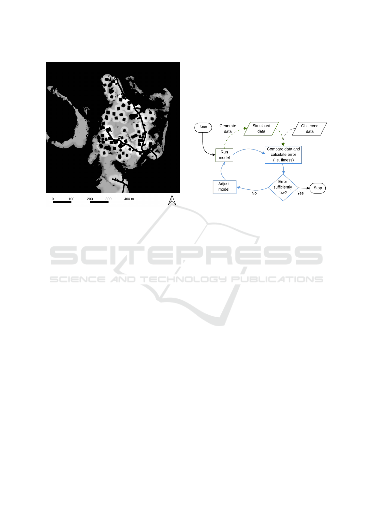
Figure 3: Aggregated Inﬂuence Map.

spots on the map without having to calculate the

whole map, which would be computationally expen-

sive as the map needs to be updated after every modi-

ﬁcation (e.g., adding a building).

3 DETERMINING PARAMETERS

OF INFLUENCE FUNCTIONS

USING A GENETIC

ALGORITHM

As previously explained, the inﬂuence sub-model is

deﬁned by a set of inﬂuences functions, their param-

eters (λ

min

, λ

and λ

max

in Equations 1-3) and their

weights for the aggregation function (i.e. the w

pa-

rameters in equation 4). To optimize these parame-

ters, the genetic algorithm NSGA-II (Deb et al., 2002)

has been chosen. It stands for “Non-dominated Sort-

ing Genetic Algorithm II” and it is widely used as a

multi-objective optimisation algorithm.

3.1 Validation Measures

Genetic algorithms need ﬁtness functions to evaluate

the accuracy of candidate solutions (in our case, pa-

rameters of the inﬂuence functions). As displayed in

Figure 4 (Crooks, 2018), measures compare the data

generated by the multi-agent model against observed

data. Then, the model is tuned, run and evaluated until

error is sufﬁciently low. Because the outcomes of the

simulations are a spatial representation of our model,

measures that take account of this spatial dimension

are needed. Three spatial measures have been chosen:

a grid-based density difference to verify that the over-

all placement of the building is more or less the same,

the Chamfer distance to quantify and summarise er-

rors into a single value, and a kernel density differ-

ence to show where the difference of density of build-

ings are.

Figure 4: The process of validation and calibration.

The grid-based density difference measure esti-

mates building density differences between simulated

and real-world data, based on a grid decomposition

of space. As illustrated in Figure 5, space is sliced

in a ﬁxed number of cells. Each cell represents a dif-

ferent area, with a certain number of buildings within

it. The centroid of the building is used to determine

the cell it belongs to. Thus, we obtain a density ma-

trix representing the number of buildings in each area.

The grid-based density difference is the absolute dif-

ference between the grid-based density matrix of real-

world data and the one of simulated data.

Formally, given two grid-based density matrices A

and B, each value of the grid-based density difference

is given by:

(A,B) =

∑

i, j

i j

− B

i j

where A

i j

and B

i j

are the number of buildings within

the cell (i, j).

The Chamfer distance is another validation mea-

sure considered in this work. It measures the differ-

ence between two point clouds. It sums the squared

distances for each point with its nearest neighbour in

the reference data set (see Figure 6). More formally,

for two non-empty subsets X and Y , the Chamfer dis-

tance d

(X,Y ) is:

(X,Y ) =

∑

x∈X

min

y∈Y

||x − y||

∑

y∈Y

min

x∈X

||x − y||

This measure will be applied to the centroids of the

buildings, and will give more information about local

differences.

ICAART 2025 - 17th International Conference on Agents and Artiﬁcial Intelligence

422

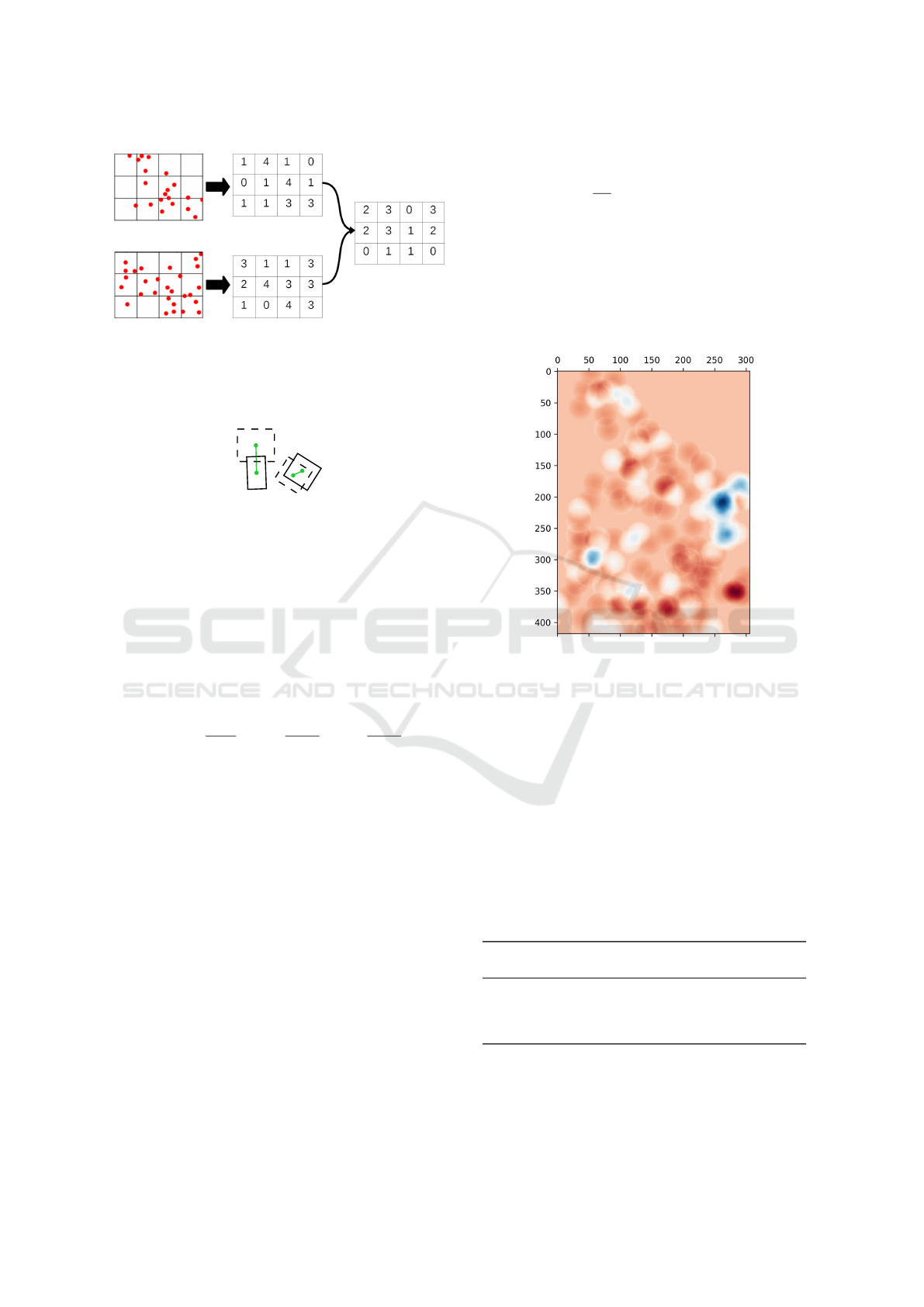
Figure 5: Example of density grid processing. The two ﬁrst

ﬁgures represent two spatial distributions of buildings (each

red point represents the centroid of a building). The two

matrices in the middle represent the number of buildings

in the corresponding cell. The last matrix is the absolute

difference of the two previous density matrices.

Figure 6: Chamfer distance example (dotted shapes are

from the validation dataset, distances are calculated be-

tween centroids).

The last validation measure studied is the kernel

density difference. It is simply the difference of two

kernel density estimations. In a GIS context, kernel

density should be more expressive/relevant than point

density, since it will smooth the density at one point

by looking at the inﬂuence of points all around. More

formally, the kernel density estimation at given coor-

dinates (x,y) is given by

f (x, y) =

n · h

∑

i=1



x − x



· K



y − y



where:

• n is the number of points,

• h is the bandwidth, which smooth the density es-

timate,

• K(u) is the kernel function, which is a symmetric

and non-negative function that integrates to 1 (in

our work, we used the Cosine kernel),

• x

and y

represent the coordinates of the ith point

in the input data set.

We process kernel density estimations for simu-

lated data and real-world ones. Then, we calculate

the difference between the two generated heat maps.

Figure 7 shows the kernel density difference between

two maps. Red areas represent a lack of buildings in

the simulation, and blue areas shows the contrary. If

the density is identical, it is displayed in white. To

use this measure as a ﬁtness function for the genetic

algorithm, we take the average of absolute differences

for each pixel in both heatmaps, i.e.:

(A,B) =

∑

i=1

∑

j=1



(i, j) −

(i, j)



where:

•

is the kernel density over the buildings cen-

troids generated by the simulation,

•

is the same but for the control dataset,

• (w,h) is the size of the bounding box of the two

combined datasets.

Figure 7: Example of Kernel Density Difference obtained

for an informal settlement located in Fiji.

4 EXPERIMENTS

4.1 Case Study

Our ﬁrst case study is an informal settlement located

near Suva, Fiji (its size is 118,885 m

). As sum-

marised in Table 1, three spatial features (buildings,

roads and paths) of this settlement have been ex-

tracted by experts using visual interpretation for four

dates (1994, 2002, 2009 and 2019).

Table 1: Spatial Features and Data Sources

Date Image Image Extracted

Type Res. Features

1994 Aerial 2.3m 61 buildings

2002 Satellite 0.8m 83 buildings and 31 roads/paths

2009 Satellite 0.59m 103 buildings and 46 roads/paths

2019 Aerial 0.35m 129 buildings and 158 roads/paths

To integrate the slope into the model, a digital el-

evation model (DEM) has been interpolated from a

digital surface model (DSM) produced during a drone

image acquisition in 2019.

Combining Procedural Generation and Genetic Algorithms to Model Urban Growth

423

4.2 Experiment Setup

Our code is developed in Python, and is available on

a GitHub repository

, along with all the data used

for the experiments. The informal settlements agent-

based model is built on top of MESA (an agent-based

modelling framework), and we used PyMOO (Blank

and Deb, 2020) for optimizing the inﬂuence function

parameters. It is a Python package that implements

multi-objectives optimisation algorithms.

As shown in the Table 2, our expert identiﬁed two

types of inﬂuence functions:

• an attraction-repulsion function for buildings and

roads;

• an open distance function for paths (because

buildings can be built on paths);

• an open distance function for slope (because a ﬂat

area is very attractive, while sloping ones are not).

Note that this function do not take a distance as in-

put, instead it takes the slope under the submitted

building.

Table 2: Genetic algorithm’s decision variables and con-

straints, associated with the inﬂuence functions.

Inﬂuence Parameters Constraints

Buildings λ

min

= X

0 ≤ X

≤ 100

(Attraction- λ

= X

+ X

0 ≤ X

≤ 100

Repulsion) λ

max

= X

+ X

0 ≤ X

≤ 100

w = X

/(X

+ X

) 0 ≤ X

≤ 1

Roads λ

min

= X

0 ≤ X

≤ 100

(Attraction- λ

= X

+ X

0 ≤ X

≤ 100

Repulsion) λ

max

= X

+ X

0 ≤ X

≤ 100

w = X

/(X

+ X

) 0 ≤ X

≤ 1

Paths λ

min

= X

0 ≤ X

≤ 100

(Open λ

max

= X

+ X

0 ≤ X

≤ 100

Distance) w = X

/(X

+ X

) 0 ≤ X

≤ 1

Slope λ

min

= X

0 ≤ X

≤ π/2

(Open λ

max

= X

0 ≤ X

≤ π/2

Distance) w = X

/(X

+ X

) 0 ≤ X

≤ 1

≤ X

Default settings of PyMOO’s NSGA-II imple-

mentation has been used. It involves a polynomial

mutation (set with a perturbation index to 20) and a

simulated binary crossover (with distribution index

set to 15 and the probability that it will happen set

to 0.9). NSGA-II population consists of 50 individu-

als, and the genetic algorithm stops when one of the

following termination criteria is met : the number of

300 generations is reached, or the objectives values

are stable for the last 30 generations.

To ﬁnd the most appropriate ﬁtness function for

NSGA-II, seven combinations of validation measures

github.com/etiennetack/spatial inﬂuences

have been tested on the three time periods of our case

study (1994 to 2002, 2002 to 2009, 2009 to 2019).

The grid-based density difference is computed using

a spatial resolution of 50m (each cell represents an

area of 50m × 50m). NSGA-II was run 50 times for

each possible combination of measures and for each

period.

4.3 Evaluating Learnt Inﬂuences

To analyse the results obtained, we ﬁrst studied the

performance of each validation measure combina-

tion. To proceed, we compared the resulting inﬂuence

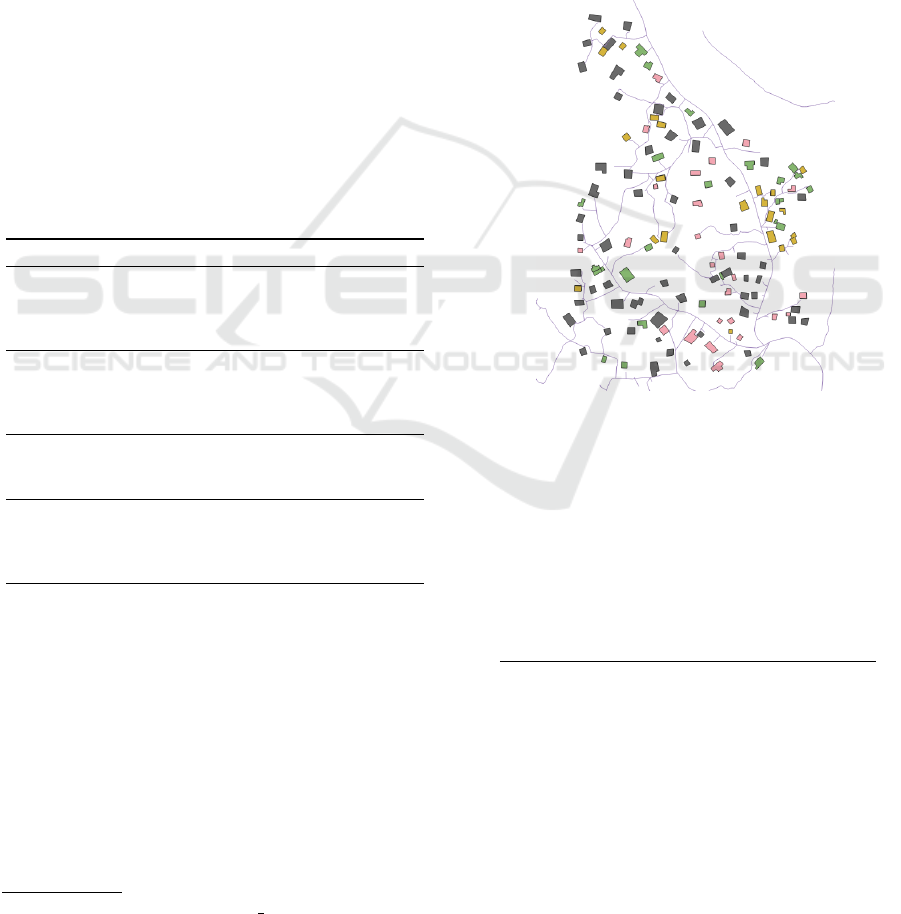
models against the real data (see Figure 8).

Figure 8: Each colour represents new buildings at each time

period: 1994 is grey, 2002 is pink, 2009 is yellow and 2019

is green.

In order to do so, we measured how many new

buildings in the ﬁeld data are placed on areas marked

as repulsive by the model (-1). These buildings high-

light errors done by the inﬂuence sub-model. There-

fore, the inﬂuence error is obtained by:

Inﬂuence Error =

Number of New Buildings On Repulsive Areas

Number of New Buildings

Figure 9 displays the mean inﬂuence error for ev-

ery validation measures combinations (i.e. ﬁtness

function in NSGA-II). As a baseline, we also calcu-

lated the inﬂuence error for random inﬂuence func-

tion parameters that comply with the same constraints

used for the genetic algorithm (see Table 2).

Those results show that NGSA-II was able to op-

timize the parameters of the inﬂuence functions in a

spatial agent-based context thanks to the chosen val-

idation measures. On average, the lowest inﬂuence

ICAART 2025 - 17th International Conference on Agents and Artiﬁcial Intelligence

424

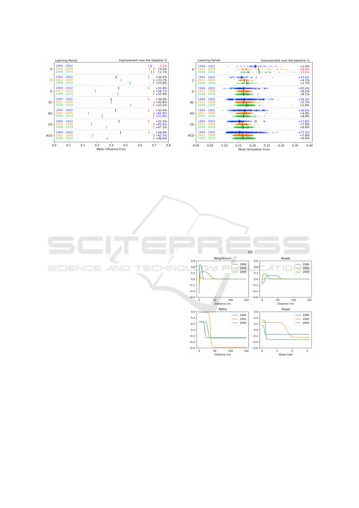
Figure 9: Application of the inﬂuence error for each mea-

sure combination and for each period.

error values are achieved using the grid-based den-

sity difference measure combined with at least an-

other measure.

4.4 Evaluating the Simulations

Although the inﬂuence error gives a good idea about

the quality of the inﬂuences functions, it does not

guarantee the realism of the resulting simulations.

Thus, a new error based on the simulation results ob-

tained using each resulting inﬂuence function set is

needed. A normalised Euclidean distance has been

used and is applied between the new buildings added

during simulation and the new buildings observed in

reality (see Table 1). One speciﬁcity when calculating

this distance is that when a validation building is se-

lected it is removed from the validation set, in such a

way that it cannot be used twice as a reference build-

ing.

As a baseline, random simulations had been con-

ducted. During those simulations, buildings are

placed randomly within the borders of the area of in-

terest without taking account of any kind of constraint

(e.g., buildings can be constructed over other build-

ings).

As shown in Figure 10, the best improvements

over random simulations are still reached using mod-

els obtained with the grid-based density difference

combined with at least another measure.

4.5 Learnt Models

Figure 11 shows the inﬂuence functions obtained with

the best combination of measures. Although the so-

lutions are near for the periods of 1994 to 2002 and

2009 to 2019, there is no unique model that works

from 1994 to 2019. The inﬂuence functions obtained

Figure 10: Simulation errors for each measure combina-

tion and each period (horizontal bars, represents the error

obtained for random simulations and the percentage num-

bers indicates the difference between the mean simulation

error of inﬂuence models and random simulations).

for 2002 are different from the two others. The in-

ﬂuence of neighbouring buildings and roads on con-

structions are low in 2002 (mainly around zero). The

inﬂuence of paths seems also more important (values

are more extreme). In 2002, the slope only has a neg-

ative inﬂuence when it is close to 2 radians (x-axis),

while this value is much lower for 1994 and 2009 (0.5

radians).

Figure 11: Inﬂuence functions for the best solutions ob-

tained with the Chamfer distance and the grid-based density

measures.

These results are still very encouraging since this

approach attempts to simulate human choices by

only considering environmental factors, while there

are other factors that inﬂuence their behaviour (e.g.

socio-economic factors).

Combining Procedural Generation and Genetic Algorithms to Model Urban Growth

425

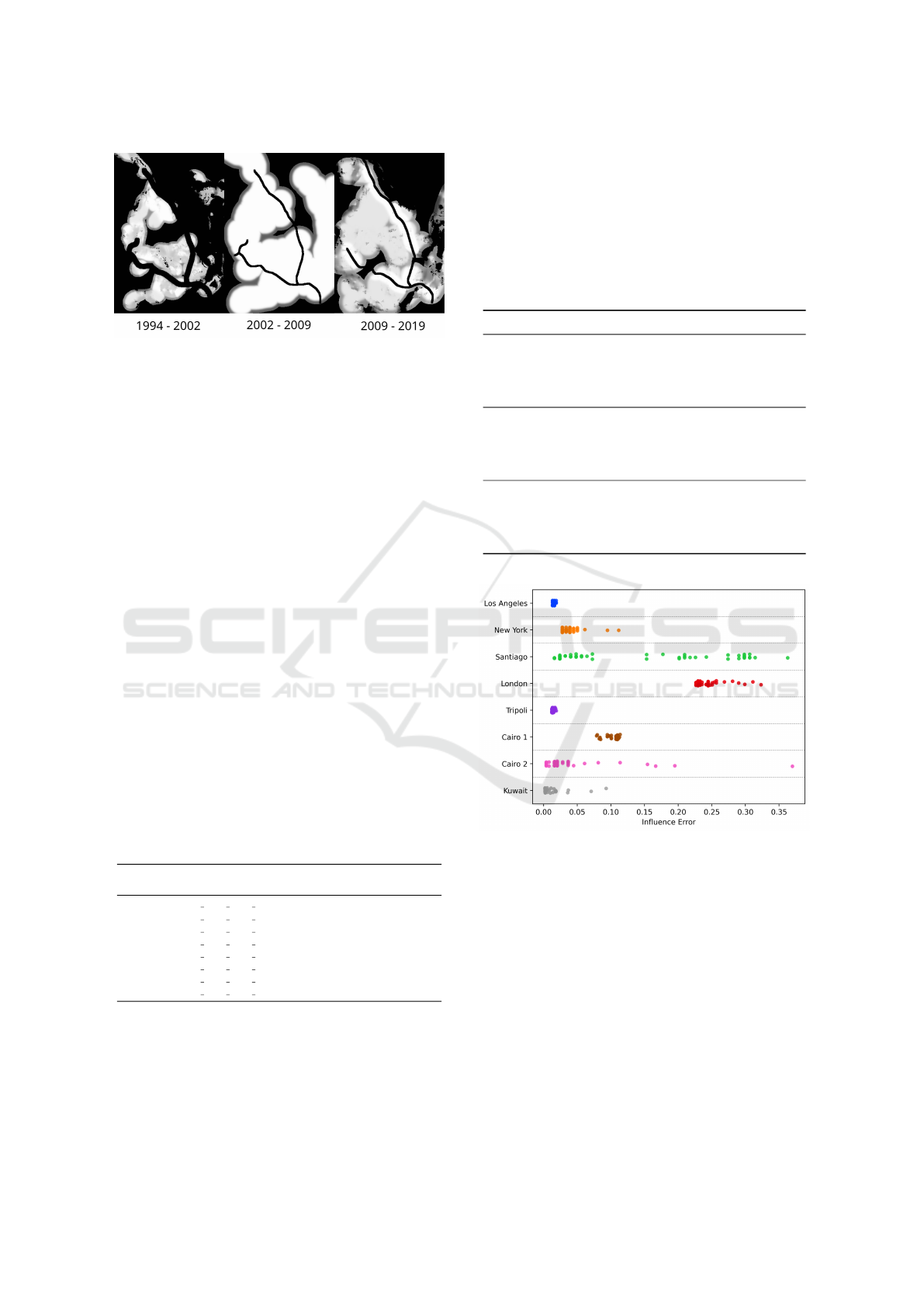
Figure 12: Inﬂuence maps of the inﬂuence functions dis-

played in the Figure 11.

5 EXPERIMENTING ON A

BROADER DATASET

To evaluate the robustness and generalisability of our

proposed urban growth model, we conducted a series

of experiments using the SpaceNet 7 dataset (Etten

et al., 2021). This dataset offers a comprehensive

collection of building footprints derived from high-

resolution satellite imagery for various cities all over

the world. providing an opportunity to test our ap-

proach on a broader and more diverse dataset com-

pared to the controlled datasets used in earlier sec-

tions of the study. This gives us larger and more

diverse datasets than those presented previously on

Suva. For this experiment, we chose data (annotated

building footprints) from cities in multiple geographic

regions. These regions vary in urban density, devel-

opment patterns, and environmental features, mak-

ing this dataset particularly suitable for stress-testing

our model’s capacity to generalize across different ur-

ban morphologies. We also speciﬁcally selected areas

where the number of building did not decrease over

time. The selected datasets, are displayed in Table 3.

Table 3: SpaceNet 7.

SpaceNet 7 Simple Size Building

Code Name (sq. km.) Delta

L15-0368E-1245N 1474 3210 13 Los Angeles 15.58 366

L15-0577E-1243N 2309 3217 13 New York 15.83 169

L15-0632E-0892N 2528 4620 13 Santiago 19.58 122

L15-1025E-1366N 4102 2726 13 London 9.37 326

L15-1138E-1216N 4553 3325 13 Tripoli 17.25 1001

L15-1203E-1203N 4815 3378 13 Cairo 1 17.96 1002

L15-1204E-1204N 4819 3372 13 Cairo 2 17.24 240

L15-1296E-1198N 5184 3399 13 Kuwait 18.38 3082

The road network data was extracted from Open-

StreetMap (OpenStreetMap contributors, 2017), pro-

viding detailed transportation infrastructure for the re-

gions in the SpaceNet 7 dataset. Additionally, we in-

corporated elevation data from the FAMDEM dataset,

allowing us to account for topographical inﬂuences on

urban growth. The genetic algorithm is still NSGA-II,

with the same parameters. We executed one training

per dataset. As shown in the Table 4, the only dif-

ference in the setup is the deletion of the paths inﬂu-

ence because there are no such footpaths in the Open-

StreetMap data.

Table 4: Learning variables and constraints for SpaceNet 7

data.

Inﬂuence Parameters Constraints

Buildings λ

min

= X

0 ≤ X

≤ 100

(Attraction- λ

= X

+ X

0 ≤ X

≤ 100

Repulsion) λ

max

= X

+ X

0 ≤ X

≤ 100

w = X

/(X

+ X

) 0 ≤ X

≤ 1

Roads λ

min

= X

0 ≤ X

≤ 100

(Attraction- λ

= X

+ X

0 ≤ X

≤ 100

Repulsion) λ

max

= X

+ X

0 ≤ X

≤ 100

w = X

/(X

+ X

) 0 ≤ X

≤ 1

Slope λ

min

= X

0 ≤ X

≤ π/2

(Open λ

max

= X

0 ≤ X

≤ π/2

Distance) w = X

/(X

+ X

) 0 ≤ X

≤ 1

≤ X

Figure 13: Inﬂuence Error SpaceNet 7.

For each city, 10 training runs were conducted,

and we then calculated the inﬂuence error and sim-

ulation error on the resulting inﬂuence models. Fig-

ure 13 illustrates the inﬂuence error for each solu-

tion obtained from the genetic algorithm. As shown

by this ﬁgure, the results of our approach on these

datasets are of the same order of magnitude as those

obtained for Suva. The simulation error (Figure 14)

yields better results. In fact, the inﬂuence error is sen-

sitive to the quality of the ﬁeld data. For example,

if the road network is not spatially accurate enough,

roads can sometimes “run over” buildings in the data.

In this case, the inﬂuence model can model that there

should be no buildings on the roads, but since this

ICAART 2025 - 17th International Conference on Agents and Artiﬁcial Intelligence

426

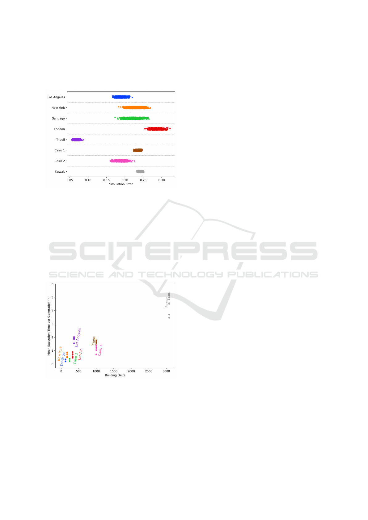
happens in the ﬁeld data, it will be counted as an er-

ror of the inﬂuence model. For example, this happens

relatively often in the London dataset, which is why

performances are worse.

Figure 14: Simulation error for SpaceNet 7.

Figure 15 illustrates the relationship between exe-

cution time per generation using one thread (in hours)

and the number of new buildings (urban growth) of

the different SpaceNet’s datasets. Naturally, the more

new buildings there are, the longer the simulation

time will be. For example, the Kuwait dataset is the

bigger, and it is associated to the longest execution

time (around 5 hours). In contrast, datasets like New

York, London, and Santiago, which have fewer build-

ings, experience much shorter execution times (under

1 hour).

Figure 15: Execution time in relation to the size of the build-

ing delta for each dataset.

6 CONCLUSIONS AND

PERSPECTIVES

This study introduces a novel approach combin-

ing procedural generation and genetic algorithms to

model spatial inﬂuences in agent-based urban growth

simulations. By formalizing environmental factors

through mathematical functions and optimizing their

parameters with NSGA-II, we generate realistic urban

growth patterns, validated using spatial measures like

grid-based density differences and Chamfer distance.

However, some notable differences between the

simulation results and the actual spatial distribution

of buildings remain. Experts believe that this is cer-

tainly due to the fact that the human factor has not

yet been taken into account in the agent-based model.

It is known in the literature that it has a strong impact

on the urban growth of such informal settlements. De-

spite these discrepancies with real-world data, our re-

sults demonstrate the method’s effectiveness and po-

tential for broader applications.

Future work will include applying the approach

to diverse regions, integrating time-series analysis

for dynamic modelling, and incorporating socio-

economic factors to better reﬂect human behaviours.

Enhancements such as generating realistic building

shapes and simulating road and path evolution are

also planned, aiming for a comprehensive, adaptable

urban modelling framework.

ACKNOWLEDGEMENTS

We would like to acknowledge the French govern-

ment having supported ﬁnancially a CIFRE doctoral

contract in collaboration with the INSIGHT company.

We also thank Thomas Gaillard (Ecosophy) and the

University of the South-Paciﬁc for the data acquisi-

tion on the site of Valenicina in Fiji, including the

Fijian students who participated during the socio-

economical survey. And more speciﬁcally, Thomas

Gaillard for his several expert returns during the mod-

elling.

REFERENCES

Agyemang, F. S. K., Silva, E., and Fox, S. (2022). Mod-

elling and simulating ‘informal urbanization’: An in-

tegrated agent-based and cellular automata model of

urban residential growth in Ghana. Environment and

Planning B: Urban Analytics and City Science.

Augustijn-Beckers, E.-W., Flacke, J., and Retsios, B.

(2011). Simulating informal settlement growth in

Dar es Salaam, Tanzania: An agent-based housing

model. Computers, Environment and Urban Systems,

35(2):93–103.

Barros, J. (2004). Simulating Urban Dynamics in Latin

American Cities. In Atkinson, P., Wu, F., Foody, G.,

Combining Procedural Generation and Genetic Algorithms to Model Urban Growth

427

and Darby, S., editors, GeoDynamics, pages 313–328.

CRC Press.

Blank, J. and Deb, K. (2020). pymoo: Multi-objective opti-

mization in python. IEEE Access, 8:89497–89509.

Crooks, A. (2018). Agent-Based Modelling and Geograph-

ical Information Systems: A Practical Primer. Spa-

tial Analysis and GIS. SAGE Publications, Thousand

Oaks, CA, 1st edition edition.

Deb, K., Pratap, A., Agarwal, S., and Meyarivan, T. (2002).

A fast and elitist multiobjective genetic algorithm:

Nsga-ii. IEEE transactions on evolutionary compu-

tation, 6(2):182–197.

Emilien, A., Bernhardt, A., Peytavie, A., Cani, M.-P., and

Galin, E. (2012). Procedural generation of villages on

arbitrary terrains. The Visual Computer, 28(6-8):809–

818.

Etten, A. V., Hogan, D., Martinez-Manso, J., Shermeyer, J.,

Weir, N., and Lewis, R. (2021). The multi-temporal

urban development spacenet dataset.

Jokar Arsanjani, J., Helbich, M., and de Noronha Vaz, E.

(2013). Spatiotemporal simulation of urban growth

patterns using agent-based modeling: The case of

Tehran. Cities, 32:33–42.

OpenStreetMap contributors (2017). Planet dump re-

trieved from https://planet.osm.org . https://www.

openstreetmap.org.

Picascia, S. and Yorke-Smith, N. (2017). Towards an

agent-based simulation of housing in urban beirut. In

Agent Based Modelling of Urban Systems, pages 3–

20. Springer International Publishing.

Schelling, T. C. (1971). Dynamic models of segregation.

Journal of mathematical sociology, 1(2):143–186.

Schwarz, N., Flacke, J., and Sliuzas, R. (2016). Modelling

the impacts of urban upgrading on population dynam-

ics. Environmental Modelling & Software, 78:150–

162.

Smelik, R. M., Tutenel, T., Bidarra, R., and Benes, B.

(2014). A survey on procedural modelling for vir-

tual worlds. In Computer Graphics Forum, volume 33,

pages 31–50. Wiley Online Library.

Tobler, W. R. (1970). A computer movie simulating urban

growth in the detroit region. Economic geography,

46(sup1):234–240.

Zhang, H., Zeng, Y., Bian, L., and Yu, X. (2010). Modelling

urban expansion using a multi agent-based model in

the city of changsha. Journal of Geographical Sci-

ences, 20:540–556.

ICAART 2025 - 17th International Conference on Agents and Artiﬁcial Intelligence

428