Integrating Machine Learning and Optimisation to Solve the
Capacitated Vehicle Routing Problem
Daniel Antunes Pedrozo
1 a
, Prateek Gupta
2
, Jorge Augusto Meira
2 b
and Fabiano Silva
1 c
1
Department of Informatics, Federal University of Paran
´
a, Brazil
2
Interdisciplinary Centre for Security, Reliability and Trust, University of Luxembourg, Luxembourg
Keywords:
Vehicle Routing Problem, Graph Attention Network, Reinforcement Learning.
Abstract:
The Capacitated Vehicle Routing Problem (CVRP) is a fundamental combinatorial optimisation challenge in
logistics. It aims to optimise routes so a fleet of vehicles can supply customer’s demands while minimising
costs - that can be seem as total distance travelled or time spent. Traditional techniques - exact algorithms,
heuristics and metaheuristics - have been thoroughly studied, but this methods often face limitations in scala-
bility and use of computational resources when confronted with larger and more complex instances. Recently,
Graph Neural Networks (GNNs) and Graph Attention Networks (GATs) have been used to tackle these more
complex instances by capturing the relational structures inherent in graph-based information. Existing meth-
ods often rely on the REINFORCE approach with baselines like the Greedy Rollout, which uses a double-
actor architecture that introduces computational overhead that could hinder scalability. This paper addresses
this problem by introducing a novel approach that uses a GAT network trained using reinforcement learning
with the DiCE estimator. By using DiCE, our method eliminates the need for a double-actor structure, which
contributes to lower the computational training cost without sacrificing solution quality. Our experiments in-
dicate that our model achieves solutions close to the optimal, with a notable decrease in training time and
resource utilisation when compared with other techniques. This work provides a more efficient machine learn-
ing framework for the CVRP.
1 INTRODUCTION
The Capacitated Vehicle Routing Problem (CVRP) is
a central combinatorial problem in logistics that fo-
cuses on determining efficient routes for a fleet of ve-
hicles to fulfill customer demands while minimising
costs (Toth et al., 2014). These costs may include total
distance travelled, time spent, or energy consumption.
Traditional methods for solving the CVRP, such as
exact algorithms, heuristics, and metaheuristics, have
been extensively studied. Exact methods like inte-
ger linear programming guarantee optimal solutions
but become computationally impractical for large in-
stances due to the problem’s NP-hard nature. Con-
versely, heuristics and metaheuristics provide approx-
imate solutions within reasonable time frames but of-
ten require specific domain knowledge (Talbi, 2009).
In recent years, machine learning techniques,
a
https://orcid.org/0009-0005-0718-3908
b
https://orcid.org/0000-0002-4086-5784
c
https://orcid.org/0000-0001-5453-6175
especially Graph Neural Networks (GNNs), have
emerged as promising tools to address the limita-
tions of traditional methods in solving combinato-
rial optimisation problems like the CVRP. GNNs
effectively capture abstract relationships in graph-
structured data, such as those between vertex at-
tributes and edge attributes (Gori et al., 2005).
Among GNN variants, Graph Attention Networks
(GATs) stand out for employing attention mecha-
nisms (Vaswani et al., 2023) to dynamically focus on
the most relevant parts of a graph, improving predic-
tions for optimal routes (Velickovic et al., 2018).
The training of neural networks for solving com-
binatorial optimisation problems is often performed
using reinforcement learning (RL) with gradient es-
timation methods (Sutton et al., 2000); (Bello et al.,
2016). The REINFORCE algorithm (Williams, 1992)
is widely used for this purpose but suffers from high
variance in gradient estimates. Implementing base-
lines, such as the Greedy Rollout (Kool et al., 2019),
can reduce this variance but at the cost of increased
computational overhead. The Greedy Rollout ap-
286
Pedrozo, D. A., Gupta, P., Meira, J. A. and Silva, F.
Integrating Machine Learning and Optimisation to Solve the Capacitated Vehicle Routing Problem.
DOI: 10.5220/0013165900003893
Paper published under CC license (CC BY-NC-ND 4.0)
In Proceedings of the 14th International Conference on Operations Research and Enterprise Systems (ICORES 2025), pages 286-293
ISBN: 978-989-758-732-0; ISSN: 2184-4372
Proceedings Copyright © 2025 by SCITEPRESS – Science and Technology Publications, Lda.

proach relies on a dual-actor architecture, where both
actor and critic parameters must be continuously up-
dated, increasing complexity.
To address these challenges, we propose a novel
approach in which a GAT is trained using RL with
the Infinitely Differentiable Monte Carlo Estimator
(DiCE) introduced by (Foerster et al., 2018). DiCE
eliminates the need for a dual-actor architecture, sig-
nificantly reducing training costs without compromis-
ing solution quality. Building on the work by (Lei
et al., 2021), we implement two variations of this ap-
proach: a straightforward replacement of the REIN-
FORCE algorithm with DiCE and a modified GAT ar-
chitecture featuring Mish activation functions (Misra,
2020) and the removal of batch normalisation layers.
These modifications aim to improve gradient flow.
Our experimental results demonstrate that the
GAT architecture trained with DiCE provides near-
optimal solutions while achieving reductions in train-
ing time and computational costs compared to tradi-
tional gradient estimation methods. These findings
suggest that the DiCE estimator offers a efficient al-
ternative for solving combinatorial problems like the
CVRP. We evaluate our approach based on solution
quality, measured by the total route distance, and
computational efficiency, assessed through memory
usage and training time.
2 LITERATURE REVIEW
The CVRP is one of the fundamental problems in
combinatorial optimisation, which aims to determine
the most efficient route for a fleet of vehicles to meet
customer demands while respecting vehicle capacity
constraints. The CVRP can be seen as an extension of
the Travelling Salesman Problem (TSP), with added
complexity through constraints like vehicle capacity.
In (Christofides, 1976), a heuristic algorithm was
proposed to solve the TSP within a distance factor of
1.5 times the optimal. Concorde solver (Applegate
et al., 2006) is widely regarded for exact solutions
to the TSP, employing cutting planes and branch-
and-bound to iteratively solve relaxed problems and
narrow the search space. Lin-Kernighan-Helsgaun
heuristic (Helsgaun, 2000) remains a state-of-the-art
heuristic for symmetric TSPs. Google’s OR-Tools
(Google, 2023) exemplifies how hand-crafted heuris-
tics combined with search algorithms can improve so-
lution quality while avoiding local optima.
The use of neural networks for combinatorial op-
timisation traces back to Hopfield and Tank (Hop-
field and Tank, 1985), who applied Hopfield networks
to solve TSP instances. Since then, neural networks
have evolved to tackle related problems. Vinyals et
al. introduced Pointer Networks (PN) (Vinyals et al.,
2017), leveraging attention mechanisms to return per-
mutations of input sets as outputs. PNs can be trained
offline to solve classes of combinatorial problems,
marking a shift in the use of deep learning to gen-
eralise solutions across different instances.
The work by (Bello et al., 2016) advanced this by
employing an Actor-Critic architecture to train PNs
without supervised data. They treated each instance
as a training example and used the route cost to esti-
mate policy gradients, achieving promising results.
Recent advances in artificial intelligence have in-
creased the adoption of neural networks for optimisa-
tion problems. GNNs (Gori et al., 2005) have become
an important tool in optimisation, preserving graph
topologies and combinatorial structures in problems
like the TSP (Dai et al., 2017). In (Battaglia et al.,
2018), the authors highlighted GNNs’ potential to
process relationally structured data by integrating re-
lational inductive biases. Velickovic et al. (Velickovic
et al., 2018) extended this by proposing Graph Atten-
tion Networks (GATs), which use attention mecha-
nisms to dynamically weigh vertices based on relative
importance, enhancing its interpretability.
In (Kool et al., 2019), the authors proposed com-
bining GATs with PNs to solve TSP and CVRP in-
stances. They introduced a reinforcement learning
framework using a simple Actor-Critic architecture,
with the REINFORCE algorithm (Williams, 1992) as
the policy estimator. Their results demonstrated near-
optimal solutions for TSP instances with up to 100
nodes. Lei et al. (Lei et al., 2021) refined this by in-
corporating edge attributes in GAT attention calcula-
tions and residual connections between neural layers
to mitigate vanishing gradients.
Despite advancements, existing methods often de-
pend on architectures with separate actor and critic
networks, increasing computational costs and limit-
ing scalability. To address this, Foerster et al. (Fo-
erster et al., 2018) introduced DiCE - an infinitely
differentiable Monte Carlo estimator. DiCE enables
unbiased gradient estimation without complex archi-
tectures, reducing variance and training time.
3 MATERIALS AND METHODS
In this section, we evaluate the performance of the
GAT trained with the DiCE estimator to solve the
CVRP. Three models are compared to analyse the ef-
fectiveness of the approach:
• Baseline Model (REINFORCE with Greedy Roll-
out): A GAT trained using the REINFORCE al-
Integrating Machine Learning and Optimisation to Solve the Capacitated Vehicle Routing Problem
287

gorithm with a Greedy Rollout baseline;
• DiCE Model: The same GAT architecture used
in the baseline model, with the training function
modified to implement DiCE; and
• DiCE
Mish
Model: An adapted GAT architecture
in which the activation functions are changed to
the Mish function and batch normalisation (BN)
layers are removed.
Our goal is to demonstrate that a GAT trained with
the DiCE estimator can provide near-optimal solu-
tions and be more computationally efficient than com-
monly used methods.
3.1 Extended GAT Model
Given an input graph G = (N, A), where N = No∪{0}
is a set composed of the union of the set of cus-
tomers, No = {1,2,..., n}, with the depot, {0}, and
A = {(i, j)|∀i, j ∈ N,i ̸= j}, is the set of all arcs con-
necting elements of N, we developed a model inspired
by the concepts presented by (Lei et al., 2021), to
solve the CVRP using both vertex and edge attributes.
Each vertex in the graph represents a customer
or the depot and is represented by its coordinates
(x
i
,y
i
) and demand q
i
, while the arcs are repre-
sented by a single attribute, the Euclidean distance
between vertices. The structure mirrors representa-
tions commonly found in previous work related to the
use of GNNs for solving combinatorial optimisation
problems, where vertices are represented by their at-
tributes, as in (Bello et al., 2016).
The objective of the implemented model is, given
an input graph g, to find a permutation of the vertices,
called a route (π), in which each vertex is visited only
once, except for the depot, n
0
, so that the total dis-
tance travelled is minimised, respecting the capacity
constraint of each vehicle:
D(
ˆ
π|s) = ||n
ˆ
π
m
−n
ˆ
π
1
||
2
+
m−1
∑
t=1
||n
ˆ
π
t
−n
ˆ
π
t+1
||
2
where ||.||
2
is the L2 norm between two vertices.
To achieve this, the neural network is trained to
learn a stochastic policy, p(π|g), that prioritises routes
with shorter distances over those resulting in longer
distances, using the chain rule for sequential process-
ing (Sutskever et al., 2014):
p(π|g) =
n
∏
t=1
p(π
t
|π
1:t−1
,g),
where, given a route π, the probability of choosing
vertex π
t
at step t is a conditional function of instance
g and previously selected vertices, π
1:t−1
.
The model follows an encoder/decoder architec-
ture and is trained following the RL paradigm. Sim-
ilar to (Kool et al., 2019), the encoder is responsible
for the embedding of the graph, concatenating the at-
tributes of the vertices with the attributes of the arcs.
The decoder then sequentially produces the route π
using the embeddings produced by the encoder and a
mask to prevent a vertex from being selected twice.
The proposed encoder takes as input a graph G =
(N, A). Each vertex in the graph represents the co-
ordinates and demand of a customer, x
i
,y
i
,q
i
, with
the demand at the depot being equal to zero. The
edges are represented by d
i j
, which denotes the Eu-
clidean distance between vertices (i, j). These at-
tributes are transformed into dimensions, d
x
and d
e
,
through a fully connected layer (FC). The final pre-
processing step before the data enters the encoder is
batch normalisation (BN). The BN aims to normalise
the outputs of the FC layers, adjusting the activations
to maintain a mean of zero and a standard deviation
of one. BN is used to reduce internal covariate shift,
thereby preventing issues of gradient imbalance.
x
(0)
i
= BN(A
0
x
i
+ b
0
),∀i ∈ N,
ˆe
i j
= BN(A
1
e
i j
+ b
1
),∀(i, j) ∈ A,
where x
i
is the embedding of vertex i and ˆe
i j
is the
embedding of edge (i, j). A
0
and A
1
are matrices
whose parameters are updated during training. The
layers are indexed as ℓ ∈ {1,...,L}, to indicate the
attributes of the vertices at a given layer ℓ. The in-
put to the first GAT layer consists of the vertex at-
tributes x
(0)
i
∈ R
d
x
,∀i ∈ N, and the edge attributes
e
i j
∈ R
d
e
,∀(i, j) ∈ A. Each GAT layer will update
the vertex attributes through the attention mechanism,
while the edge attributes remain unchanged. The at-
tention coefficient, α
i j
, indicates the importance of
vertex j to vertex i. The attention mechanism is cal-
culated as follows:
α
(ℓ)
i j
=
exp

σ

g
ℓ
T
[W
ℓ
(x
(ℓ−1)
i
|x
(ℓ−1)
j
|ˆe
i j
)]

∑
n
z=1
exp

σ

g
ℓ
T
[W
ℓ
(x
(ℓ−1)
i
|x
(ℓ−1)
z
|ˆe
iz
)]

Here, g
ℓ
and W
ℓ
are parameterizable vectors and ma-
trices, respectively, σ(·) is the activation function,
LeakyReLU, and ·|·|· is a concatenation operation.
The activation function LeakyReLU assigns a
small gradient to negative inputs, ensuring that the
GAT can learn even when activations are less than
zero. This prevents neurons from outputting zero
and, consequently, their gradients from becoming
zero. If a neuron’s gradient becomes zero, it will no
longer contribute to the network’s learning. More-
over, LeakyReLU is computationally simpler, which
increases the efficiency of larger neural networks.
ICORES 2025 - 14th International Conference on Operations Research and Enterprise Systems
288

The output of layer ℓ, if ℓ ̸= L, is given by the
concatenation of the vertex attributes obtained from
the previous layer and the attributes updated by the
attention mechanism in the current layer:
x
(ℓ)
i
= x
(ℓ−1)
i
+
n
∑
j=1
α
(ℓ)
i j
W
ℓ
1
x
(ℓ−1)
j
,
refers to this as a residual connection. Residual con-
nections function by adding their input to the output
of the current layer’s processing, enhancing training
stability and preventing gradients from becoming so
small that they no longer contribute to learning.
The final layer of the encoder, layer L, outputs the
attributes of each vertex, x
(L)
i
, which are used to con-
struct the graph representation, a vector that encapsu-
lates all the information in the graph, using the fol-
lowing function: ¯x
j
=
1
n
∑
n
i=1
(x
(L)
i
)
j
, j ∈ {1,..., d
x
}.
The graph representation is, therefore, given by the
average of the vertex attributes from the final layer
across all vertices, ¯x = {¯x
1
,..., ¯x
d
x
}, ¯x
j
∈ R.
The implemented decoder is based on the model
proposed by (Vaswani et al., 2023) and utilises a
multi-head attention mechanism (MHA). In conjunc-
tion with the MHA, a Pointer Network (PN) (Vinyals
et al., 2017) is also implemented, as it enables the
use of a transformer model to handle combinatorial
problems. The PN assigns a probability to each ver-
tex, which is used at each step to determine the po-
sition in the input set of the selected vertex that will
compose the route. Thus, the size of the input set de-
fines the size of the GAT’s output set. Following the
model of (Lei et al., 2021), this implementation does
not use batch normalisation, residual connections, or
fully connected layers in the decoder.
The decoder consists of two attention layers. De-
coding occurs sequentially, and at each step t ∈
{1,..., n}, the decoder presents a vertex to form the
route,
ˆ
π
t
, based on the vector representation received
from the encoder and previous decodings
ˆ
π
t
′
, t
′
< t.
The first layer of the decoder is composed of an
MHA (with H heads) that receives a context vector,
c
(0)
t
, as input and produces a new context vector, c
(1)
t
.
The context vector c
(0)
t
is constructed by concatenat-
ing the graph representation received from the en-
coder, ¯x , the last vertex chosen by the decoder,
ˆ
π
t−1
,
and the first selected vertex,
ˆ
π
1
.
The MHA involves three essential components:
query vectors q; key vectors k; and value vectors v.
The query vector is obtained by transforming the con-
text vector c
(0)
t
using a parameterizable matrix, W
Q
.
The key and value vectors are obtained by transform-
ing the vertex vector representations x
(L)
i
using param-
eterizable matrices W
K
and W
V
, respectively. The di-
mension of these vectors is given by d
v
= (d
x
/H):
q = W
Q
c
(0)
t
, W
Q
∈ R
d
v
×d
x
,
v
i
= W
V
x
(L)
i
, W
V
∈ R
d
v
×d
x
, i ∈ {1, 2,..., n},
k
i
= W
K
x
(L)
i
, W
K
∈ R
d
v
×d
x
, i ∈ {1, 2,..., n}.
The query and key vectors are used to compute the
attention coefficient, u
(1)
i,t
, by combining them, where
u
(1)
i,t
=
q
T
k
i
√
d
v
, if vertex i has not yet been selected, and
−∞ otherwise. Indicating that the attention coefficient
of a given vertex i is equal to −∞ effectively masks i
so that it is not selected again during the iteration. To
ensure that the attention coefficients are normalised,
the softmax function is applied, transforming them
into a probability distribution that indicates the im-
portance of each vertex within the attention context.
This process is repeated H times, each with a dif-
ferent set of parameters, forming the MHA. The result
of each process is then concatenated in sequence and
used to compute the resulting context vector of the
first decoder layer, c
(1)
t
, through a FC layer:
c
(1)
t
= W
f
·




H
h=1
n
∑
i=1
( ˆu
(1)
i,t
)
h
(v
h
i
)

The use of the MHA allows the model to enhance
its representational power, capturing more complex
patterns present in the input data by considering them
from different perspectives.
The context vector c
(1)
t
serves as the input to the
second decoder layer. This layer consists of a sim-
ple attention mechanism that calculates new attention
coefficients, ˆu
(2)
i,t
∈ R, ∀i ∈ {1,.. .,n}:
u
(2)
i,t
=



C ·tanh

c
(1)
t
k
i
√
d
v

,if i ̸=
ˆ
π
t
′
∀t
′
< t.
−∞ ,otherwise.
As proposed by (Bello et al., 2016), (Lei et al.,
2021) also opted to limit the range of possible val-
ues for the attention coefficients ˆu
(2)
i,t
to [−C,C ]. The
new attention coefficients are then used to calculate
the probability distribution for each vertex at a given
time t: p
i,t
= p
θ
(
ˆ
π
t
|s,
ˆ
π
t
′
, ∀t
′
< t) = softmax(u
(2)
i,t
).
This probability distribution is used to select which
vertex
ˆ
π
t
to include in the route.
The training of the baseline model was carried
out using the REINFORCE algorithm with a Greedy
Rollout Baseline (GR), inspired by the work of (Kool
et al., 2019). The REINFORCE algorithm is a
Monte Carlo method that estimates the policy gra-
dients π
θ
(A
t
|S
t
) through sampling, with the base-
line acting to minimise the variance produced by the
Integrating Machine Learning and Optimisation to Solve the Capacitated Vehicle Routing Problem
289

method. The Loss function, L(θ|s), is defined as the
expected reward of the policy π
θ
given an instance
s: L(θ|s) = Eπ
θ
[R(
ˆ
π|s)], where R(
ˆ
π|s) represents the
reward for a given route
ˆ
π. The gradient of the Loss
function is then estimated using the REINFORCE al-
gorithm with a baseline b(s) to minimise the variance:
∇
θ
L(θ|s) = E
π
θ
(
ˆ
π|s)
[(R(
ˆ
π|s) −b(s))∇
θ
logπ
θ
(
ˆ
π|s)]
In our model, the GR strategy acts as a baseline in
which the policy greedily selects the vertices to com-
pose the route based on the highest probability at each
decision point. This policy is executed by running a
second actor (GAT) pass, but in deterministic mode,
in a structure called dual-actor.
At the end of each epoch, the actor is evaluated
on a set of validation instances, and the result is com-
pared with the results obtained through the GR. If the
learned policy of the actor is significantly superior to
the deterministic result, the baseline parameters are
updated according to the actor’s parameters. This en-
sures that the model is always tested against a signifi-
cant baseline, stimulating performance gains.
Additionally, the same GAT model was trained
using the DiCE method, which offers a more stable
way to calculate gradients in the context of RL for
combinatorial optimisation problems. DiCE aims to
address issues caused by high variance and incorrect
calculation of higher-order gradients, common in esti-
mators such as REINFORCE. By using the structure
of stochastic computation graphs (SCG) (Schulman
et al., 2016), the DiCE technique ensures that the cor-
rect dependency relationship between stochastic ver-
tices, such as the choices made by the policy (actor),
and cost vertices, the objective function, such as the
total distance travelled, is maintained throughout the
SCG. By avoiding the break in dependency relation-
ships between the SCG vertices, DiCE can compute
higher-order gradients, improving model convergence
by increasing the precision of the policy’s parameter
updates (Foerster et al., 2018).
Finally, The DiCE
Mish
model, aiming to enhance
the estimator’s capabilities, was modified to allow
better gradient propagation through the neural net-
work structure during backpropagation for parame-
ter adjustments. Thus, the non-linear activation func-
tions LeakyReLU and Tanh were replaced by the Mish
function Mish(x) = x.tanh(ln(1 + e
x
)) (Misra, 2020)
and the BN layers were removed.
3.2 Metrics
The work presents four metrics to evaluate the perfor-
mance of the methods applied to solving the CVRP:
average distance; average distance relative to the un-
trained model; average time; and total time. The av-
erage distance corresponds to the total distance trav-
elled across all test instances relative to the total num-
ber of tested instances. This metric aims to com-
pare the quality of the solutions found by each model.
The average distance relative to the untrained model
aims to present the percentage distance of each neu-
ral network-based model tested relative to the result
before training. The average time to solution acts as
a proxy to compare the computational efficiency of
GAT-based approaches. The total time represents the
sum of the time spent by the techniques used to solve
each instance.
4 EXPERIMENTS
The focus of this work is to compare the results ob-
tained from different training strategies GATs to solve
the CVRP. The GAT architectures used follow the
principles from the works presented by (Kool et al.,
2019) and (Lei et al., 2021), and can therefore, with
minimal alterations to the employed mask, input data,
and decoder processing, be used to solve other combi-
natorial problems, such as routing problem variations.
All models were developed, trained, and tested in
the following configuration: a 13th-generation Intel
processor with 10 cores (2.5GHz) and 32GB of RAM;
and an Nvidia GTX 1660 Super graphics card with
6GB of memory for parallel processing.
The deep learning models were trained using two
RL strategies: gradient calculation using the REIN-
FORCE algorithm with a baseline based on a GR
of the actor, and gradient estimation using the DiCE
estimator. In this second strategy, two architectures
were employed. The first used the same architecture
as in the training under REINFORCE. The second
underwent minor changes to allow unrestricted gra-
dient propagation, replacing the activation functions
LeakyReLU and Tanh with Mish and removing the BN
layer from the encoder structure.
The hyperparameters used in the training were
kept constant across all trainings performed, as shown
in Table 1. The training instances were randomly gen-
erated with 21 vertices (customers plus depot) each,
with the coordinates of each vertex belonging to the
interval given by [1.0] x [1.0]. In total, 768,000 in-
stances were used in batches of 512, with training
conducted over one hundred epochs, 1500 iterations
per epoch, totalling 150,000 training steps.
As a base for comparison we used the exact solver
with a basic implementation of the CVRP
1
to serve
1
Developed using the SCIP framework in Python.
ICORES 2025 - 14th International Conference on Operations Research and Enterprise Systems
290

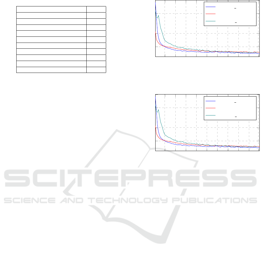
Table 1: Hyperparameters used in training.
Hyperparameter Value
Input Vertex Dimension 3
Input Edge Dimension 1
Vertex Embedding Dimension 128
Edge Embedding Dimension 16
Layers in Encoder 4
Negative Slope - LeakyReLU 0.2
Dropout Rate 0.6
Decoder Iterations 100
Learning Rate (LR) 1e-4
SOFTMAX Temperature (T) 2.5
as a baseline for comparing the sub-optimal solutions.
For that, we use two distinct datasets for testing. First,
a synthetic set of one hundred problem instances with
ten customers each was created, following the in-
stance generation process used for the training data.
This dataset was constructed to enable the compari-
son of the solutions obtained by the GAT approach
with those found by the exact solver.
A second synthetic dataset of one hundred in-
stances with twenty customers each was created to
compare the quality of the solutions and response
times among the deep learning models. This sec-
ond test aims to compare the different strategies em-
ployed: REINFORCE with GR, DiCE, and DiCE
Mish
.
4.1 Training
This section provides an analysis of the training per-
formance differences among the implemented GAT
models. The models differ primarily in the choice of
gradient estimator used. The objective is to analyse
the implementations with respect to learning conver-
gence per training epoch.
Figure 2 shows the evolution of the reward value
(objective function result) over the training epochs of
the three implemented GAT models: Greedy Rollout,
DiCE, and DiCE
Mish
. The vertical axis represents the
value of the objective function (reward), while the
horizontal axis represents the number of epochs. It
can be observed that all models converge rapidly up
to the twentieth epoch, after which the learning pro-
cess becomes more stable. It is worth noting that the
REINFORCE method using GR shows slightly supe-
rior performance in terms of convergence speed.
It is also important to highlight a significant dif-
ference between the DiCE models and the GR model.
The implementations that use DiCE as the gradient
estimator do not employ a dual-actor architecture, as
seen in the GR, where the second actor serves as a
critic. By avoiding the need for a second network to
act as a critic, the DiCE implementation significantly
reduces computational overhead, making it more effi-
10 20 30 40
50 60
70 80 90 99
10
12
15
17
Epoch
Reward
Greedy Rollout
DiCE
DiCE Mish
Figure 1: Reward per Epoch for Different Implementations.
10 20 30 40
50 60
70 80 90 99
10
12
15
17
Epoch
Reward
Greedy Rollout
DiCE
DiCE Mish
Figure 2: Reward per Epoch for Different Implementations.
cient. Additionally, the DiCE architecture has lower
computational complexity, as the dual-actor structure
of the GR model requires both the actor and the critic
to be continuously optimised, whereas DiCE opti-
mises only a single actor.
This difference becomes evident when comparing
the total time required for training. To train for one
hundred epochs, the GR model required 20.52 hours,
approximately 738 seconds per epoch. In contrast, the
DiCE model took only 14.24 hours, or 512 seconds
per epoch. Finally, the DiCE
Mish
implementation took
14 hours to train for one hundred epochs, or 504 sec-
onds per epoch. It can be seen that the architectures
employing the DiCE estimator offer advantages in re-
ducing total training time without compromising the
quality of the presented solution.
4.2 Comparison with the Exact Method
In this section, the performance of the implemented
GAT architecture models in solving the CVRP is
compared to the solutions presented by the exact
method. Evaluations are performed based on three
metrics: average distance travelled, average distance
relative to the optimal solution, and total time spent.
The test instances were randomly generated using a
Integrating Machine Learning and Optimisation to Solve the Capacitated Vehicle Routing Problem
291

Table 2: Comparison with the exact method: 10 customers.
Model Avg. distance Dist. rel. to opt. (%) Total time (s)
GAT Base 7.48 71.5 8.38
DiCE Mish 4.59 5.33 0.80
DiCE 4.60 5.47 0.56
GR (Greedy Rollout) 4.53 4.32 0.65
SCIP (Exact) 4.36 0.00 (Optimal) 0.67
Table 3: Comparison between deep learning models: 20 customers.
Model Avg. distance Dist. rel. to GR (%) Total time (s) Time rel. to GAT Base (%)
GAT Base 15.10 - 4.93 -
DiCE Mish 7.13 0.46 3.84 22.12
DiCE 7.16 0.89 4.05 17.85
GR (Greedy Rollout) 7.10 0.00 (Baseline) 4.23 14.17
set of ten customers and three vehicles.
The first metric, average distance travelled, repre-
sents the average distance of the routes generated by
each model over a set of one hundred test instances.
As shown in Table 2, which presents the average per-
formance of all models, the exact method achieves
the shortest average distance, as expected. Except
for the result presented by the pre-trained model,
“GAT Base”, the models generated by deep learn-
ing do not exhibit significant variations among them-
selves, presenting results overall very close to the op-
timal solution.
Table 2 allows for a precise evaluation of the per-
centage variation between the solutions presented by
the models. The row GAT base shows the result ob-
tained by the model prior to training and, as expected,
it is significantly worse than the other approaches.
The Greedy Rollout strategy presents a result only
4.3% higher than that of the exact method. It should
be noted that the other techniques also present very
similar results, with the DiCE
Mish
model being only
1% superior to the deterministic model.
Finally, Table 2 shows the total time spent to solve
one hundred test instances, each with ten customers.
The image confirms that solving the CVRP using an
exact method requires significantly more time com-
pared to the deep learning models.
4.3 Comparison Between Models
In this section, we compare the performance of the
implemented GAT architecture models in solving the
CVRP. Evaluations are performed based on four met-
rics: average distance travelled, average distance rel-
ative to the Greedy Rollout model solution, total time
spent, and time relative to the untrained model. The
test instances were randomly generated using a set of
twenty customers.
The values presented in Table 3 shows the aver-
age distance travelled by each model in solving one
hundred instances, each with twenty customers. It
can be observed that the trained models — Greedy
Rollout, DiCE, and DiCE
Mish
— produce very simi-
lar values. Among them, the model trained with the
REINFORCE algorithm using a GR baseline showed
the lowest average value of 7.0951. The DiCE
Mish
ar-
chitecture achieved the second-best result at 7.1279,
with the DiCE architecture trailing at 7.1584.
Table 3 provides a deeper comparison between the
models by showing the relative difference of the av-
erage solutions compared to that obtained by the GR
model. The scale is presented in logarithmic form to
improve visualisation of the differences between the
values. The significant difference observed between
the untrained model and the trained models suggests
that the GATs were able to capture the necessary pat-
terns for solving the CVRP. It is worth noting that the
small difference between the average solution value
found by the DiCE
Mish
model and the value of the GR
model can be considered non-significant. Among the
trained models, DiCE
Mish
exhibited the shortest total
time, at 3.84 seconds. The DiCE model took 4.05 sec-
onds to solve the one hundred instances, while the GR
model required the most time, at 4.23 seconds.
To highlight the difference in time taken by the
models to solve the problem, Table 3 shows the so-
lution time of the trained models relative to the un-
trained model for the one hundred test instances. It
can be observed that the GR model, while faster than
the baseline, solving the instances in 14.2% less time,
is slower than the DiCE architectures. The difference
is majored when compared to the DiC E
Mish
model,
which was 22.1% faster than the untrained model in
solving the test set. It is evident that the DiCE
Mish
model, in addition to demonstrating good perfor-
mance in solving the CVRP in terms of time, provides
ICORES 2025 - 14th International Conference on Operations Research and Enterprise Systems
292

near-optimal solutions in terms of cost (7.13). Cou-
pled with only a 0.46% difference relative to the GR
model, the DiCE
Mish
model emerges as an efficient
alternative for routing problems, balancing solution
quality with computational efficiency.
5 CONCLUSION AND FUTURE
WORK
This work presented a novel approach for solving the
CVRP using GATs trained under the RL paradigm
employing the DiCE estimator. Our primary contri-
bution is the elimination of the need for a dual-actor
structure, which is commonly employed in traditional
methods like REINFORCE with a GR baseline, re-
sulting in lower computational costs without compro-
mising the quality of the solutions.
The experiments indicate that by using the DiCE
estimator, the developed GAT models obtain near-
optimal solutions while reducing training time and
computational costs compared to more traditional
techniques, such as the actor-critic model. Specifi-
cally, the architectures employing the DiCE estimator
showed training times approximately 30% lower than
the time spent by REINFORCE with Greedy Roll-
out. Moreover, the DiCE method not only makes the
model more efficient in terms of time but also sim-
plifies the training process by eliminating the need to
optimise both an actor and a critic simultaneously.
This line of research opens up important chal-
lenges for exploration in future work. One signifi-
cant development would be the implementation of a
warm-start strategy, which has the potential to reduce
the computation time of exact models by providing
sub-optimal solution values during initialisation. This
strategy is particularly relevant in large-scale optimi-
sation operations, where a good initial solution can
significantly reduce the problem’s search space. Ad-
ditionally, combining traditional optimisation tech-
niques, such as dynamic programming and branch
and bound, with machine learning models could lead
to the creation of hybrid solutions that leverage the
strengths of each approach. Finally, techniques such
as Transfer Learning could be used to apply knowl-
edge gained from solving smaller or less complex in-
stances to larger or more complex ones without re-
quiring new training.
REFERENCES
Applegate, D. L., Bixby, R. E., Chv
´
atal, V., and Cook, W. J.
(2006). The traveling salesman problem. http://www.
math.uwaterloo.ca/tsp/concorde.html. Accessed: Oc-
tober, 2023.
Battaglia, P. W., Hamrick, J. B., Bapst, V., Sanchez-
Gonzalez, A., Zambaldi, V., Malinowski, M., Tac-
chetti, A., Raposo, D., Santoro, A., Faulkner, R., et al.
(2018). Relational inductive biases, deep learning, and
graph networks. arXiv preprint arXiv:1806.01261.
Bello, I., Pham, H., Le, Q. V., Norouzi, M., and Bengio, S.
(2016). Neural combinatorial optimization with rein-
forcement learning. CoRR, abs/1611.09940.
Christofides, N. (1976). Worst-case analysis of a new
heuristic for the travelling salesman problem. (388).
Dai, H., Khalil, E. B., Zhang, Y., Dilkina, B., and Song,
L. (2017). Learning combinatorial optimization algo-
rithms over graphs. CoRR, abs/1704.01665.
Foerster, J., Farquhar, G., Al-Shedivat, M., Rockt
¨
aschel, T.,
Xing, E. P., and Whiteson, S. (2018). Dice: The in-
finitely differentiable monte-carlo estimator.
Google (2023). Or-tools. https://developers.google.com/
optimization. Accessed: October, 2023.
Gori, M., Monfardini, G., and Scarselli, F. (2005). A new
model for learning in graph domains. 2:729–734 vol.
2.
Helsgaun, K. (2000). An effective implementation of the
lin–kernighan traveling salesman heuristic. European
Journal of Operational Research, 126(1):106–130.
Hopfield, J. and Tank, D. (1985). Neural computation of
decisions in optimization problems. Biological cyber-
netics, 52:141–52.
Kool, W., van Hoof, H., and Welling, M. (2019). Attention,
learn to solve routing problems!
Lei, K., Guo, P., Wang, Y., Wu, X., and Zhao, W. (2021).
Solve routing problems with a residual edge-graph at-
tention neural network. CoRR, abs/2105.02730.
Misra, D. (2020). Mish: A self regularized non-monotonic
activation function.
Schulman, J., Heess, N., Weber, T., and Abbeel, P.
(2016). Gradient estimation using stochastic compu-
tation graphs.
Sutskever, I., Vinyals, O., and Le, Q. V. (2014). Sequence
to sequence learning with neural networks.
Sutton, R. S., Mcallester, D., Singh, S., and Mansour, Y.
(2000). Policy gradient methods for reinforcement
learning with function approximation. 12:1057–1063.
Talbi, E.-G. (2009). Metaheuristics: From Design to Imple-
mentation. Wiley Publishing.
Toth, P., Vigo, D., Toth, P., and Vigo, D. (2014). Vehicle
Routing: Problems, Methods, and Applications, Sec-
ond Edition. Society for Industrial and Applied Math-
ematics, USA.
Vaswani, A., Shazeer, N., Parmar, N., Uszkoreit, J., Jones,
L., Gomez, A. N., Kaiser, L., and Polosukhin, I.
(2023). Attention is all you need.
Velickovic, P., Cucurull, G., Casanova, A., Romero, A., Li
`
o,
P., and Bengio, Y. (2018). Graph attention networks.
ArXiv, abs/1710.10903.
Vinyals, O., Fortunato, M., and Jaitly, N. (2017). Pointer
networks.
Williams, R. J. (1992). Simple statistical gradient-following
algorithms for connectionist reinforcement learning.
Machine Learning, 8:229–256.
Integrating Machine Learning and Optimisation to Solve the Capacitated Vehicle Routing Problem
293