AI-Accelerated Viewshed Computation for High-Resolution Elevation

Models

edric Schwencke, Dominik St

utz and Dimitri Bulatov

Fraunhofer IOSB Ettlingen, Gutleuthausstrasse 1, 76275 Ettlingen, Germany

Keywords:

Viewshed Computation, Visibility Analysis, Neural Networks, Digital Terrain Models, Digital Surface

Models, Supervised Learning, GIS, Environmental Monitoring.

Abstract:

Viewshed computation, essential for visibility analysis in GIS applications, involves determining visible areas

from a given point using the digital terrain model (DTM) and digital surface model (DSM). The traditional

methods, though accurate, can be computationally intensive, especially with increasing search distances and

high-resolution elevation DSMs. This paper introduces a novel approach leveraging neural networks to es-

timate the farthest visible point (FVP). At this point the viewshed computation could be aborted, which sig-

niﬁcantly reducing computation time without compromising accuracy. The proposed method employs a fully

connected neural network trained on varied terrain proﬁles, achieving over 99% accuracy in visibility predic-

tions while reducing the required amount of computations by more than 90%. This approach demonstrates

substantial performance gains, making it suitable for applications requiring fast visibility analysis.

1 MOTIVATION

The computation of viewshed in outdoor point clouds,

which are often sampled into more manageable

DSMs, has numerous applications. For instance, ac-

cording to (Pan et al., 2020), viewshed analysis can

distinguish visible and invisible areas from a DSM in

mountainous areas and determine the suitability of re-

gions for forest tourism practices (Lee et al., 2019;

Hognogi et al., 2022). Viewshed computation is

also applicable in aquatic and marine systems (Arnon

et al., 2023; Qiang et al., 2019). Additionally, it can

predict the velocity expansion of sound waves or po-

tentially dangerous gases, aiding in decision-making

processes.

Despite the efﬁciency of viewshed analysis for a

single viewpoint, the processing time becomes signif-

icant when calculating multiple viewpoints, known as

total-viewshed computation. Moreover, the computa-

tion time increases dramatically with a growing max-

imum view distance or higher resolution. For many

applications, a large or nearly inﬁnite view distance is

necessary.

In this paper, we focus on improving a total-

viewshed computation algorithm based on line of

sight (LoS). LoSs are used for simpliﬁcation. To

speed up the viewshed computation on each LoS, we

introduce a novel approach. We estimate the FVP on

https://orcid.org/0000-0002-0560-2591

a LoS to abort the visibility computation earlier. An

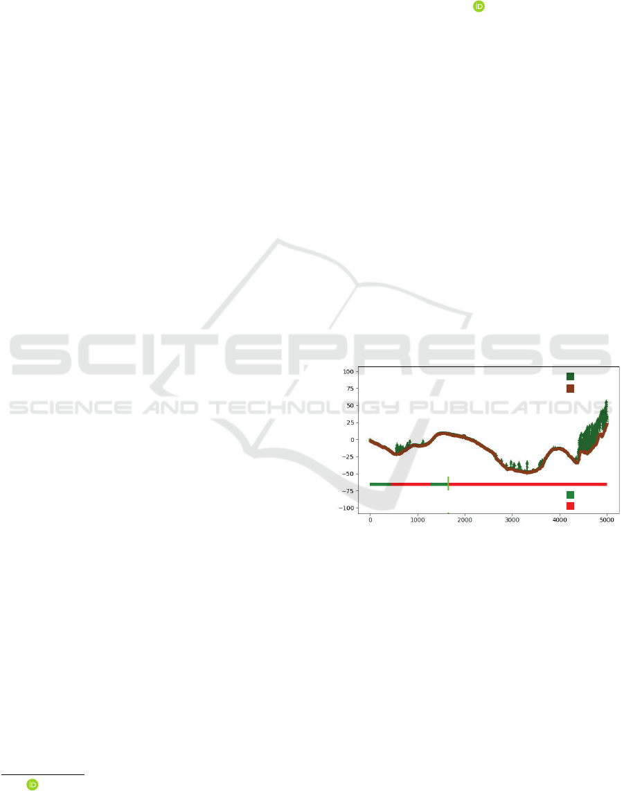
example of a LoS in proﬁle view is shown in Figure

Distance to the observer [m]

DSM

DTM

Visible

Invisible

Relative height to the observer [m]

FVP

Figure 1: This graph illustrates the visibility of a target

(1.9m high), placed on the DTM, from the observer’s per-

spective along the LoS. The brown line represents the DTM,

while the green areas indicate the DSM. The visibility is de-

picted through a straight line at the bottom: red indicates in-

visible segments, and green indicates visible segments. The

vertical bright green line marks the FVP that remains visi-

ble from the observer’s location.

Deﬁning a hard cutoff criterion, such as rough-

ness, is challenging due to the variety of topogra-

phies. Although the computation of a single LoS re-

quires few operations, it is challenging to undercut

this for the cutoff criterion. Humans can intuitively

and quickly assess the necessary extent of viewshed

computations when examining terrain proﬁles, inspir-

ing the use of a neural network to estimate the FVP.

Schwencke, C., Stütz, D. and Bulatov, D.

AI-Accelerated Viewshed Computation for High-Resolution Elevation Models.

DOI: 10.5220/0013168400003912

Paper published under CC license (CC BY-NC-ND 4.0)

In Proceedings of the 20th International Joint Conference on Computer Vision, Imaging and Computer Graphics Theory and Applications (VISIGRAPP 2025) - Volume 1: GRAPP, HUCAPP

and IVAPP, pages 251-258

ISBN: 978-989-758-728-3; ISSN: 2184-4321

251

Parallelizing the computation using multiple LoSs

makes fully connected networks promising for per-

formance enhancement. The output of the neural net-

work may either exceed or fall short of the true value

of the FVP. In the former case, unnecessary computa-

tion resources are used, but the result remains correct.

In the latter case, computation resources are saved at

the risk of errors.

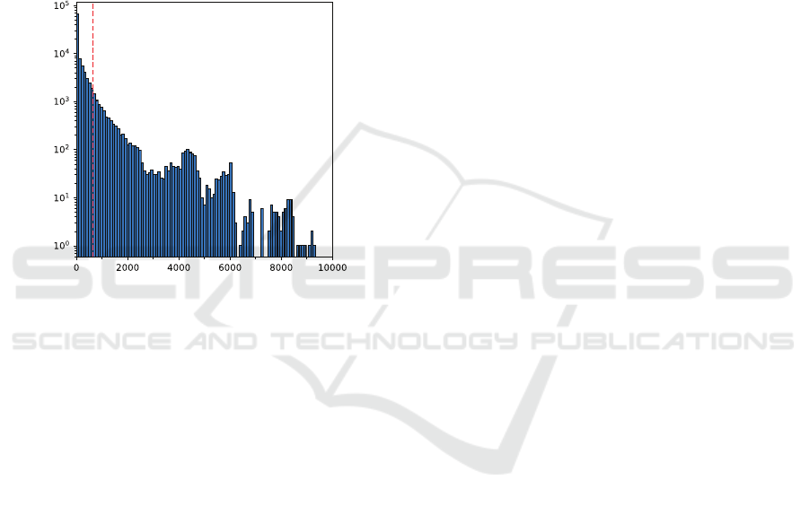
As illustrated in Figure 2, for 90% of the LoS, the

furthest visible point is within a distance of 1000m

towards the observer. Therefore, it is often unneces-

sary to calculate the entire LoS for a correct viewshed

result.

Distance to FVP [m]

Number of LoS

90% Percentile

Figure 2: Histogram over distances to the FVP on a LoS,

visible by an observer. The data samples were taken across

all datasets described in Section 4.

In Section 2, we provide a comprehensive

overview of related work to accelerate viewshed com-

putation. Our proposed method is introduced in Sec-

tion 3. We describe the datasets used, present the re-

sults, and draw the main conclusions in Sections 4, 5,

and 6, respectively.

2 RELATED WORK

This section provides an overview of notable methods

for total Viewshed computation and explores innova-

tive strategies for enhancing computational efﬁciency.

Within at least a quarter-of-century, the ﬁeld of

Viewshed computation has been explored intensively

regarding increased efﬁciency. To begin with, (Stew-

art, 1998) proposed a fast algorithm for computing

the horizon at all sample points in a digital elevation

map, demonstrating improved accuracy and speed,

particularly for terrains with over 100 000 sample

points, making it suitable for visibility culling and

rendering. Building on this, (Tabik et al., 2013) in-

troduced a novel algorithm that computes the total-

viewshed for all points in a terrain simultaneously,

signiﬁcantly outperforming traditional GIS viewshed

tools by combining visible heights and low-cost com-

putations. (Tabik et al., 2015)’s work emphasized efﬁ-

ciency through effective data structures and high data

reuse across multiple viewpoints. Similarly, (Qarah,

2020) developed a parallel GPU algorithm utilizing

a radial-sweep approach, achieving remarkable speed

improvements over traditional CPU-based methods,

while (Pan et al., 2020) recommended the Matryoshka

doll algorithm to enhance computation efﬁciency in

viewshed analysis. Based on (Tabik et al., 2015),

(Sanchez-Fernandez et al., 2021) further contributed

to the ﬁeld with their skewed digital elevation model

(sDEM), which improved memory access locality in

rotational sweep algorithms, demonstrating substan-

tial speedups compared to conventional GIS soft-

ware. The application of visibility-based path plan-

ning heuristics by (Sanchez-Fernandez et al., 2022)

showcased the potential of total-viewshed computa-

tion for maximizing visual coverage in UAV mon-

itoring tasks. (Heyns and Van Vuuren, 2013) fo-

cused on facility placement optimization based on

viewshed visibility percentages, proposing methods

to estimate viewshed efﬁciently with minimal accu-

racy loss. (Wang et al., 2023) introduced an inno-

vative algorithm that computes viewshed using ref-

erence planes, resulting in signiﬁcant reductions in

computing time compared to traditional LoS based

methods. Recently, (Arnon et al., 2023) presented

ViewShedR, an open-source tool designed for cumu-

lative, subtractive, and elevated LoS analyses, facili-

tating accessibility for scholars in environmental and

ecological studies. (Parent and Lei-Parent, 2023) de-

veloped a 2D viewshed approach that utilizes land

cover to estimate visibility extents, proving effective

for large study areas where trees and buildings serve

as primary obstacles. Lastly, (Zhang et al., 2021) in-

troduced a Spark-based parallel computing approach

for the XDraw algorithm, signiﬁcantly enhancing ef-

ﬁciency and scalability in Viewshed analysis for high-

resolution raster DSM.

Collectively, these contributions highlight the on-

going evolution and innovation in viewshed computa-

tion. We continue this by pursuing a novel approach

that signiﬁcantly reduces the initial computation ef-

fort by intelligently estimating the FVP for the ﬁrst

time.

GRAPP 2025 - 20th International Conference on Computer Graphics Theory and Applications

252

3 METHODOLOGY

This section outlines the methodology used to speed

up the viewshed computation using neural networks.

We begin with an overview of the conventional

method, followed by the introduction of an AI-based

approach. Detailed descriptions of the network archi-

tecture, training data, and the loss function are pro-

vided subsequently.

3.1 Preliminaries

A viewshed computation method described by

aufel et al., 2023) use LoS. Key terms of this

method are described in Figure 3. This method cal-

culates the viewshed of a target (t) from an observer

(o) as:

:= DTM(o) + h

(1)

:= DTM(t) + h

(2)

where h

is the observer and h

the target height. To

calculate the viewshed of a target on the LoS, the

maximum slope variable S

∗

is initialized to −∞. On

the LoS, the distance from the target towards the ob-

server ρ = [1, .., D] is deﬁned, where ρ

is the distance

to the target and D the maximum visibility distance.

The current LoS slope S is computed for every target

position as:

S := max



− z

DSM(t) − z



(3)

The boolean visibility on the LoS v

and the maxi-

mum slope S

∗

are updated according to:

If S > S

∗

: v

:= 1 and S

∗

:= S else v

:= 0. (4)

3.2 Viewshed-AI Architecture

Human intuition allows a quick estimation of the

FVP in terrain proﬁles, which is in most cases much

smaller than D. Inspired by this, we propose using

a neural network to estimate the FVP and relinquish

the viewshed computation on the LoS much further

afar, whereby “much´´ means a safety margin to be

imposed is recommendable, as we will see later. In ei-

ther way, doing so would massively reduce the com-

putation expense while maintaining accuracy, espe-

cially when parallelized over multiple LoSs.

The procedure is schematically explained in Fig-

ure 4 with hypothetical numerical in- and outputs. We

employ a fully connected neural network, consisting

of an input layer, hidden layers with ReLU activation

functions, and dropout layers. The input layer gets the

concatenated proﬁles of the normalized digital sur-

face model (nDSM) and the DTM. Additionally, the

Observer

Target

LoS

DSM

DTM

Bird's Eye View

Prole view

Observer

Visibility

FVP

Figure 3: Key terms related to viewshed computation using

LoS. It depicts the observer’s location, the target being eval-

uated, and the LoS that indicate visibility. The DSM and

DTM are essential for determining visibility. The viewshed

represents the area visible from the observer’s point. The

ﬁgure includes both a bird’s eye view, showcasing the ter-

rain and visibility relationships from above, and a proﬁle

view, illustrating elevation changes and sight lines. Green

and Red colors along the LoS marks areas where the orange

target is (in-) visible from the observer.

target height value is appended. The network’s ﬁnal

layer outputs the predicted FVP.

Distance

to FVP

521

nDSM

DTM

Target

height

1.8

Neural

Network

Figure 4: The process for estimating the FVP. The input

data in the gray box consists of a nDSM, a DTM adjusted

for observer height, and the target height. A neural network

processes this information to determine the FVP. The nu-

meric values shown are illustrative examples.

The number of neurons in hidden layers and

dropout rates can be adjusted to the problem. This

network reliably learns relationships within a vector

and has a very short evaluation time. The architecture

is chosen to balance evaluation time and accuracy, ini-

tially focusing on feed-forward networks.

3.3 Training Data

Training data is created by selecting random strips

of length l from our DTMs and the corresponding

DSMs. Each strip includes an observer and target

height chosen in range 0.5 m to 4.0 m.

The network’s input layer receives a vector con-

taining the DTM, nDSM, and target height. The input

AI-Accelerated Viewshed Computation for High-Resolution Elevation Models

253

vector is structured as.

[ DTM | nDSM | Target Height ] .

with an input dimension of D = 2l + 1. Hereby, the

nDSM denotes normalized DSM, which is the eleva-

tion over the ground, or the difference between DSM

and DTM. Furthermore, the DTM and nDSM are sub-

tracted towards the absolute observer height to make

their values relative towards him.

The training dataset contains the input vector, vis-

ibility at each point, and the calculated FVP, see Fig-

ure 3. The FVP is generated by determining the slope

between z

and z

and comparing it with the maxi-

mum slope from previous points.

3.4 Loss Function

The loss function inﬂuences the network’s training by

weighting errors.

Underestimating ρ

∗

should be penalized much

more than overestimating this variable. The latter

would result in the necessity of making more com-

putations during viewshed computation, which is a

smaller threat than the former, that is, overlooking po-

tentially visible points, because it may signify a par-

ticular value or alarm. Our function should be some-

how skewed towards positive differences between ac-

tual and predicted values of ρ

∗

Another way to encourage rather farther visibility

is to impose scale invariance and proportional error

measurement. To this end, we based our function on

the Huber loss, which is quadratic for small and linear

for large deviations between actual and predicted val-

ues. Our modiﬁed Huber loss L : N × N × {0, 1}

→

≥0

with user-speciﬁed parameters β, γ, and δ is de-

ﬁned by Equation (5).

L(x, ρ

∗

, v) =













−



if δ < L

if 0 ≤ L

≤ δ,

βŁ

+ γL

if − δ ≤ −L

< 0,

δβ



−L

−



+ γL

otherwise,

where L

= x − ρ

∗

and L

∗

∑

i=x

(5)

In this loss function, x is the FVP generated by the

network, ρ

∗

is the actual FVP, v indicates visibility

at each point (1 is visible, 0 is invisible), and x

max(x, 0). The vector v is hereafter called truth vec-

tor. The parameter β weights the loss for x − ρ

∗

< 0,

δ controls the interval for quadratic deviations, and γ

adds a penalty for unconsidered visibility.

The choice of β, δ, and γ inﬂuences the balance

between computation time and error minimization.

An optimal set of parameters minimizes early FVP

errors while maximizing computation efﬁciency. We

will turn to this issue during the ablation study. How-

ever, in short, δ is the trade-off between linear and

quadratic error, typical for the Huber function, β is the

skewing parameter for negative x − ρ

∗

, and γ allows

taking into account the number of points for which

visibility was incorrectly predicted.

4 DATASETS

The proposed method can be trained and tested for

any dataset for which DSM and DTM are available.

Of course, the more diverse datasets exist, the more

generalized the output model is. We considered three

datasets from our repository, which cover a range

from very ﬂat to hilly terrain. They originate from

three European regions: Karsava in Eastern Latvia,

Altm

ulltal is in Bavaria in Southern Germany, and

Wetter is in the province of Hesse in Central Germany.

Latvian dataset is quite ﬂat and has quite many forest

regions. Bavaria is a bit hilly, and Hesse even more

so. The dataset from Bavaria, also referred to as Gred-

ing, was used by other scientiﬁc publications, such as

(Kuester et al., 2021). Key parameters for describing

the terrain of the three datasets can be seen in Figure

5. The resulting dataset contains an equal amount of

every region, which can ensure a sufﬁcient diversity

in the data.

The considered height proﬁles start at arbitrary

points in the dataset and extend in arbitrary directions,

each measuring a length of 10000m. Through sam-

pling in different directions, the variety can be further

increased. Some 10% of them were used for training

and the rest validating the algorithm.

Absolute DTM dierence [m]

Median nDSM height [m]

Median DTM slope [°]

Median DSM roughness

Latvia Bavaria Hesse

Figure 5: Parameters of considered datasets.

GRAPP 2025 - 20th International Conference on Computer Graphics Theory and Applications

254

5 RESULTS

To assess the performance of the network, we

straightforwardly measure the absolute error between

the predicted and actual FVP. Besides, we want to

track the relative performance accuracy ε of the truth

vector v, using the same notation as in (5):

ε = 1 −

∗

∑

i=x

, (6)

with l describing the length of the LoS. The reason to

take it into consideration lies in the later application.

The higher number of visible points after the gener-

ated stop leads to a higher error. If the ρ

∗

leads to an

early stop with only a few visible points much further

along the LoS, the saved time could be more beneﬁ-

cial.

With these considerations in mind, we will discuss

network designs, qualitative and quantitative ﬁndings,

as well as a comparison with the conventional View-

shed Algorithm, optionally accelerated with a max-

slope criterion, in the remainder of this section.

5.1 Ablation Study

In this section, we will consider a few network de-

signs and provide experiments with different network

parameters. We chose four networks with different

amounts of layers and neurons because we aim for a

fast inference method, whilst maintaining a high ac-

curacy.

Table 1: Number of neurons in reviewed network architec-

tures with parameters (β, γ, δ) = (2, 100, 500).

Layer-Number →

Network-ID ↓ 1 2 3 4

1 2048 1024 512 —

2 1024 512 256 —

3 2048 1024 512 256

4 1024 512 256 128

As can be seen in Figure 6a, all four networks

produce similar results; networks with three layers

overshoot more than those with four. Otherwise, hav-

ing 2048 neurons in the ﬁrst hidden layer results in

a lower deviation of absolute errors. This behavior is

desired; nevertheless, a higher number of neurons and

layers leads to a longer evaluation time. A suitable

network has to be chosen according to the speciﬁcs of

the application. While experimenting with different

parameters, some tendencies could be derived. In-

creasing the value of β results in a higher deviation

of the errors, while shifting the mean upwards. This

behavior should be expected, as the network tends to

overestimate the FVP value due to the composition of

the loss function. Adjusting the parameters γ or δ does

not change the outcome as much as expected. A cor-

relation between those parameters needs to be further

investigated. Overall, it is not possible to come to a

ﬁnal conclusion because the mutual dependencies of

the parameters have proven to be relatively complex.

Error [m]

Relative accuracy

Network Network

(a)

Error [m]

Relative accuracy

Latvia Bavaria Hesse Latvia Bavaria Hesse

(b)

Figure 6: Box plots of errors and accuracy ε for the net-

works mentioned in Table 1 (a) and for the different regions

(b). The black lines indicate the quantile deviation between

the 5% and the 95% quantile. The gray box depicts the in-

terquartile range, and the green line shows the median. The

red dots represent the empirical mean.

5.2 Qualitative Evaluation

The results discussed from now on were generated

with network-ID 3 from Table 1. This network rep-

resents a suitable choice according to the hyperpa-

rameter optimization framework Optuna (Akiba et al.,

2019). Afterward, the network design has been

slightly modiﬁed based on empirical observations. In

Figure 7, we can observe six examples (at the top)

in which the network predicts the FVP with an ex-

tremely high accuracy, while three examples on the

bottom exhibit different kinds of deviations. In the

successful examples of the FVP retrieval, the second

row shows a few challenging situations. It can be ob-

served that despite some FVPs being far away or not

on top of a hill, the network predicts the FVP with a

high accuracy. The least pleasant for our application

errors of too early FVPs happen occasionally close

to the forests, although there are some vertical slopes

further away. The most FVP errors of our applica-

AI-Accelerated Viewshed Computation for High-Resolution Elevation Models

255

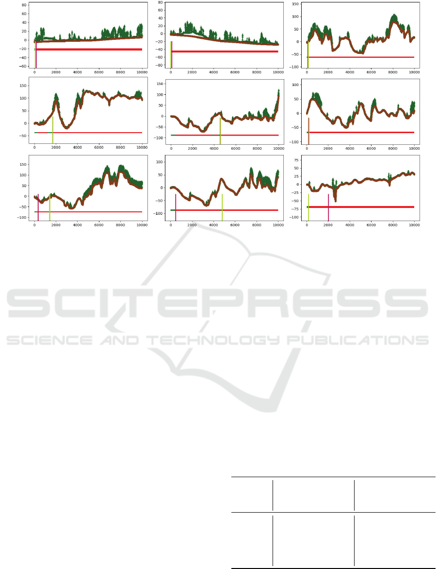
Figure 7: Examples of six correctly predicted FVPs (accuracy ε over 99%, top two rows) and two incorrectly predicted FVPs

(bottom rows, accuracy ε below 90%). Vertical green and purple bars indicate the actual and predicted points The elevation

proﬁles in the DSM and DTM are shown in green and brown. Observed and non-observed points are represented by green

and red fragments, respectively, in the horizontal line below.

tion occur occasionally near forests, although there

are some vertical slopes further away. Fortunately, in

the majority of these cases, only a few actually visible

points are missed.

5.3 Quantitative Assessment

In this section, we discuss the accuracy produced by

the aforementioned network. From Figure 2 it be-

comes clear that in the elevation proﬁles along the

10000m, some 90% of the deviations constitute less

than 250m. The accuracy of the truth vector exceeds

97% for 95% of the test data. Our network is able

to estimate the approximate position of the FVP. It is

also not critical to achieve a slightly too early FVP be-

cause a safety margin of around 250m, barely notice-

able in the application of the method in Section 3.1,

can be added. The accuracy of our network is ±250m,

which might seem modest but represents only 2% of

the total visibility range of 10000m. By adding this

2% as a safety margin, we achieve no errors in 90% of

the cases. Unfortunately, the errors are unevenly dis-

tributed in three different regions, as becomes evident

from Figure 6b. In Latvia, the results are much more

accurate than in Bavaria. This indicates that the net-

work produces better outputs for ﬂatter regions. Per-

formance of the method in very mountainous regions

is yet to be tested.

5.4 Comparison with Max-Slope

Criterion in Terms of Time and

Accuracy

Table 2 represents the percentage of needed computa-

tions compared to an implementation with no abort

condition, along with the achieved accuracy. For

comparison, two other abort criteria are displayed.

Those abort the computation if the regarded view an-

gle between the observer height and a point on the

DSM exceeds a certain threshold. The network is dis-

played with different safety margins.

Table 2: Percentage of computations needed using different

FVP criteria, compared to no FVP criterion for Latvia (L),

Bavaria (B), and Hesse (H). We denote in the left-most col-

umn network 3 from Table 1 by N3.

FVP- Computations mean Accuracy

crit. ↓ [%] [%]

Region → L B H L B H

◦

7.82 19.53 11.48 99.99 99.82 99.80

◦

38.65 53.98 46.68 99.99 99.99 99.99

N3 1.02 4.00 5.30 99.69 99.51 99.75

N3[+250] 3.42 6.40 7.7 99.90 99.82 99.91

N3[+500] 5.92 8.90 10.20 99.96 99.91 99.95

Using the network-generated FVP for aborting re-

duces the amount of computations quite signiﬁcantly.

Implementing a simple criterion like an angle-based

GRAPP 2025 - 20th International Conference on Computer Graphics Theory and Applications

256

abort condition is a much simpler strategy and can

also reduce the number of computations. Although

the angle-based criteria with a 15

◦

condition lead to

a near-perfect accuracy, it may fail depending on the

terrain regarded. We can see that Karsava in Latvia

has so many trees and so many quite short values for

FVP, that the simple strategy to abort as soon as 1

◦

slope is achieved is very difﬁcult to beat in terms of

accuracy. A high deviation of absolute errors, seen in

Figure 6b, leads to a signiﬁcantly higher percentage

of needed computations. But also for other regions,

the 1

◦

max slope criterion can only be outperformed

only by means of a safety margin, and at a cost of

necessary computations. However, in Table 2, we dis-

played the mean values, which are susceptible for the

outliers. Taking into account the 5% quantile, the 1

◦

criterion achieves 0.99 for Latvia, but 0.98 for Bavaria

and Hesse. The network with a safety margin of 250

achieves 1 for Latvia and Hesse and 0.99 for Bavaria.

This is why the apparently good performance of the

simple max slope criterion is misleading.

Overall, the computing time is hardware- and

implementation-dependent. With an Intel

Xeon

Gold 6154 CPU, the time needed to infer the FVP for

one LoS is approximately 0.03ms, when the input-

data contains 10000 LoSs.

6 CONCLUSION

In this paper, we presented a novel approach to accel-

erate the viewshed computation. For each LoS, the

FVP is estimated, after which the viewshed compu-

tation is aborted. Before the FVP the viewshed com-

putation is exactly as before. Ideally, this results in

no loss of accuracy compared to traditional methods.

Since the distance towards the FVP is signiﬁcantly

smaller than the desired maximum visibility distance,

in most cases substantial speed gains can be achieved.

We achieve an accuracy of ±250m. Our test data

shows that we could save more than 90% of the com-

putations, whilst maintaining a high accuracy when

dealing with large viewshed distances or high resolu-

tion datasets. This efﬁciency cannot be achieved by

traditional LoS algorithms and even with the simple

◦

criterion, we achieved much less points to be tested

with comparable accuracy.

As this is our initial study with this approach, we

are conﬁdent that further improvements in accuracy

and speed are achievable. There are many possibil-

ities within network architecture, making it unlikely

that we have found the optimal solution in the ﬁrst

attempt.

In future studies, we aim to enhance performance

through skip connections or parallel network architec-

tures. Additionally, we plan to investigate the aptitude

of convolutional neural networks. Deeper networks

are not currently planned due to performance consid-

erations.

ACKNOWLEDGEMENTS

Freely available AI-based text generation techniques

helped summarize Section 2. The sources were se-

lected by the authors who also carefully double-

checked the resulting text. We also thank the review-

ers for their insightful comments.

REFERENCES

Akiba, T., Sano, S., Yanase, T., Ohta, T., and Koyama, M.

(2019). Optuna: A next-generation hyperparameter

optimization framework. In Proceedings of the 25th

ACM SIGKDD International Conference on Knowl-

edge Discovery and Data Mining.

Arnon, E., Uzan, A., Handel, M., Cain, S., Toledo, S.,

and Spiegel, O. (2023). Viewshedr: a new open-

source tool for cumulative, subtractive and elevated

line-of-sight analysis. Royal Society Open Science,

10(6):221333.

aufel, G., Bulatov, D., Emter, T., Frese, C., Kottler, B.,

Petereit, J., Schmidt, A., Solbrig, P., St

utz, D., and

Wernerus, P. (2023). Ghost: Getting invisibly from

position A to position B. In Emerging Imaging and

Sensing Technologies for Security and Defence VIII,

volume 12740, pages 32–43. SPIE.

Heyns, A. and Van Vuuren, J. (2013). Terrain visibility-

dependent facility location through fast dynamic step-

distance viewshed estimation within a raster environ-

ment. In Proceedings of the Conference of the Oper-

ations Research Society of South Africa, pages 112–

121. Operations Research Society of South Africa.

Hognogi, G.-G., Pop, A.-M., M

aescu, S., and Nistor, M.-

M. (2022). Increasing territorial planning activities

through viewshed analysis. Geocarto International,

37(2):627–637.

Kuester, J., Gross, W., and Middelmann, W. (2021). 1D-

convolutional autoencoder based hyperspectral data

compression. The International Archives of the Pho-

togrammetry, Remote Sensing and Spatial Informa-

tion Sciences, 43:15–21.

Lee, K. Y., Seo, J. I., Kim, K.-N., Lee, Y., Kweon, H.,

and Kim, J. (2019). Application of viewshed and spa-

tial aesthetic analyses to forest practices for mountain

scenery improvement in the Republic of Korea. Sus-

tainability, 11(9):2687.

Pan, Z., Tang, J., Tjahjadi, T., Wu, Z., and Xiao, X.

(2020). A novel rapid method for viewshed com-

putation on dem through max-pooling and min-

AI-Accelerated Viewshed Computation for High-Resolution Elevation Models

257

expected height. ISPRS International Journal of Geo-

Information, 9(11):633.

Parent, J. R. and Lei-Parent, Q. (2023). Rapid viewshed

analyses: A case study with visibilities limited by

trees and buildings. Applied Geography, 154:102942.

Qarah, F. F. (2020). Efﬁcient viewshed computation algo-

rithms on GPUs and CPUs. PhD Thesis at the Uni-

versity of South Florida.

Qiang, Y., Shen, S., and Chen, Q. (2019). Visibility analysis

of oceanic blue space using digital elevation models.

Landscape and Urban Planning, 181:92–102.

Sanchez-Fernandez, A. J., Romero, L. F., Bandera, G.,

and Tabik, S. (2021). A data relocation approach

for terrain surface analysis on multi-gpu systems: a

case study on the total viewshed problem. Interna-

tional Journal of Geographical Information Science,

35(8):1500–1520.

Sanchez-Fernandez, A. J., Romero, L. F., Bandera, G., and

Tabik, S. (2022). Vpp: Visibility-based path planning

heuristic for monitoring large regions of complex ter-

rain using a uav onboard camera. IEEE Journal of Se-

lected Topics in Applied Earth Observations and Re-

mote Sensing, 15:944–955.

Stewart, A. J. (1998). Fast horizon computation at all

points of a terrain with visibility and shading applica-

tions. IEEE Transactions on Visualization and Com-

puter Graphics, 4(1):82–93.

Tabik, S., Cervilla, A. R., Zapata, E., and Romero, L. F.

(2015). Efﬁcient data structure and highly scalable al-

gorithm for total-viewshed computation. IEEE Jour-

nal of Selected Topics in Applied Earth Observations

and Remote Sensing, 8(1):304–310.

Tabik, S., Zapata, E., and Romero, L. (2013). Simultane-

ous computation of total viewshed on large high res-

olution grids. International Journal of Geographical

Information Science, 27(4):804–814.

Wang, Z., Xiong, L., Guo, Z., Zhang, W., and Tang, G.

(2023). A view-tree method to compute viewsheds

from digital elevation models. International Journal

of Geographical Information Science, 37(1):68–87.

Zhang, J., Zhao, S., and Ye, Z. (2021). Spark-Enabled

XDraw viewshed analysis. IEEE Journal of Selected

Topics in Applied Earth Observations and Remote

Sensing, 14:2017–2029.

GRAPP 2025 - 20th International Conference on Computer Graphics Theory and Applications

258