Analyzing Cognitive Patterns in Gifted Children Using MRI and

Morphometric Similarity Networks

Shuning Han

1,2 a

, Feng Duan

3 b

, Gemma Vilaseca

4,5 c

, N

uria Vilar

5 d

, Cesar F. Caiafa

6 e

Zhe Sun

2,7 f

and Jordi Sol

e-Casals

1,8 g

Data and Signal Processing Research Group, University of Vic-Central University of Catalonia, Vic, Catalonia, Spain

Image Processing Research Group, RIKEN Center for Advanced Photonics, RIKEN, Wako-Shi, Saitama, Japan

Tianjin Key Laboratory of Brain Science and Intelligent Rehabilitation, Nankai University, Tianjin, China

Psychological Department, Oms and Prat school, Fundaci

o Catalunya - La Pedrera, Manresa, Catalonia, Spain

Oms Foundation, Manresa, Catalonia, Spain

Instituto Argentino de Radioastronom

ıa-CCT La Plata, CONICET / CIC-PBA / UNLP, Argentina

Faculty of Health Data Science, Juntendo University, Urayasu, Chiba, Japan

Department of Psychiatry, University of Cambridge, Cambridge, U.K.

Keywords:

Gifted Children, Structural Magnetic Resonance Imaging, Morphometric Similarity Network, Connection

Density, Anatomical Modularity, Topological Features.

Abstract:

Advances in non-invasive neuroimaging, such as structural magnetic resonance imaging (sMRI), have en-

abled the construction of structural brain networks (SBNs), allowing in vivo mapping of anatomical connec-

tions. This study investigates brain network structural differences linked to different intelligence levels in

children by individual morphometric similarity networks (MSNs) derived from sMRI data. Through group-

and individual-level analyses, we aim to uncover key topological features associated with cognitive perfor-

mance and to identify a suitable connection density for SBN analysis. Connection density strongly affects

global and nodal topological features, with a range of p = 0.05 to 0.15 recommended for stable and optimal

results. Gifted individuals exhibit stronger intra-hemispheric and intra-modular connectivity, a more balanced

distribution of left-to-right intra-hemispheric connections, and lower mean versatility, supporting efﬁcient and

stable cognitive processing. Moreover, anatomical modularity analyses based on von Economo indicate that

higher cognitive performance is linked to enhanced connectivity in speciﬁc areas (such as secondary sensory

area, motor to association area and secondary sensory to limbic area), alongside selective reduction in cer-

tain modular connections (such as motor to insular area, association to secondary sensory area and motor to

secondary sensory area). Furthermore, topological features, including participation coefﬁcient and local efﬁ-

ciency, are linked to cognitive performance. These ﬁndings provide valuable insights into the SBNs underlying

cognitive levels in children.

1 INTRODUCTION

Understanding the neural basis of cognitive abilities

has long been a key goal in cognitive neuroscience.

Despite considerable progress, signiﬁcant gaps re-

main, particularly in understanding the structural and

functional differences in the brains of gifted individ-

https://orcid.org/0009-0004-0792-5484

https://orcid.org/0000-0002-2179-2460

https://orcid.org/0000-0002-7533-2355

https://orcid.org/0000-0002-7273-6039

https://orcid.org/0000-0001-5437-6095

https://orcid.org/0000-0002-6531-0769

https://orcid.org/0000-0002-6534-1979

uals. A promising approach to bridging this gap is

the study of brain networks, which explores the con-

nectivity and interactions among different brain re-

gions. Recent advances in non-invasive neuroimag-

ing techniques, such as structural magnetic resonance

imaging (sMRI) and diffusion MRI, have enabled re-

searchers to map these anatomical connections in vivo

(Genon et al., 2022; Lo et al., 2011). These techniques

allow for the construction of structural brain networks

(SBNs), where the brain is modeled as a graph com-

posed of nodes (brain regions) and edges (connections

between them), providing a foundation for applying

graph theory to explore the brain’s organization and

its relationship to cognitive abilities (Faskowitz et al.,

Han, S., Duan, F., Vilaseca, G., Vilaró, N., Caiafa, C. F., Sun, Z. and Solé-Casals, J.

Analyzing Cognitive Patterns in Gifted Children Using MRI and Morphometric Similarity Networks.

DOI: 10.5220/0013169200003911

Paper published under CC license (CC BY-NC-ND 4.0)

In Proceedings of the 18th International Joint Conference on Biomedical Engineering Systems and Technologies (BIOSTEC 2025) - Volume 1, pages 729-740

ISBN: 978-989-758-731-3; ISSN: 2184-4305

729

2022).

Two main approaches are used to construct SBNs:

tractography from diffusion-weighted imaging (DWI)

and structural covariance networks (SCNs) derived

from sMRI. SCNs traditionally compute the covari-

ance of a single morphometric feature, such as corti-

cal thickness, between regions across a group of sub-

jects (Sol

e-Casals et al., 2019). While this method

has been invaluable in understanding group-level

brain organization, recent advances have introduced

individual-level SCNs, allowing for a more detailed,

personalized view of brain structure by incorporating

multiple morphometric features (Kong et al., 2015;

Li et al., 2017; Yu et al., 2018; Seidlitz et al., 2018;

Li et al., 2021; Sebenius et al., 2023; Sun et al.,

2024a,b). A notable development in this ﬁeld is

the morphometric similarity network (MSN) (Seidlitz

et al., 2018), which constructs individual brain net-

works using multiple structural features derived from

sMRI. MSNs are based on the pairwise correlations

of morphometric feature vectors between brain re-

gions, facilitating a more granular investigation of

the brain’s structural organization. This method has

shown promise in revealing biologically relevant pat-

terns in brain networks.

Previous research has uncovered distinct patterns

in SBNs associated with various biological charac-

teristics, such as gender (Sun et al., 2015), cogni-

tive ability (Park and Friston, 2013) and neurode-

generative diseases progression (Sun et al., 2024b).

Despite these advances, key questions remain unan-

swered. How do the topological properties of MSNs

relate to cognitive performance, particularly in chil-

dren? How do modular and hemispheric specializa-

tions contribute to neural efﬁciency in gifted individ-

uals? How do different connection densities affect

brain network properties? These questions are criti-

cal for understanding the structural underpinnings of

cognitive abilities.

This study addresses these gaps by constructing

MSNs from sMRI data and analyzing their topo-

logical features in relation to cognitive performance

in both gifted and control groups. Speciﬁcally, we

conduct a comprehensive group comparison analy-

sis, focusing on modular connections based on von

Economo (VE) (Von Economo, 1929), the effects

of different connection densities, intra-/inter-modular

connections based on VE and intra-/inter-hemispheric

connections. We also explore how nodal, global topo-

logical features and speciﬁc VE-Region connections

are linked to cognitive performance. By combining

group-level and individual-level analyses, this study

offers new insights into the neural mechanisms of

giftedness, emphasizing the role of anatomical mod-

ularity, hemispheric specialization, and topological

features in efﬁcient cognitive processing.

The rest of this paper is structured as follows: Sec-

tion 2 outlines the dataset and methods employed.

Section 3 presents the results of our analyses, which

are discussed in Section 4. Finally, Section 5 con-

cludes the study.

2 MATERIALS AND METHODS

2.1 Data

2.1.1 Participants

In this study, we use the dataset consisting of sMRI

and cognitive tests from 29 healthy right-handed male

participants with no history of psychiatric or neu-

rological disorders (Sol

e-Casals et al., 2019). The

raw (anonymized) MRI data and cortical thickness

data are accessible in the OpenNeuro repository at

https://openneuro.org/datasets/ds001988.

The participants are categorized into two groups:

a control group (CG, 14 subjects) and a gifted group

(GG, 15 subjects). Details of the participants’ infor-

mation can be found in Table 1. The table indicates no

signiﬁcant age differences but signiﬁcant difference

in full-scale IQ between the groups.

Table 1: Participant information.

Groups CG (Mean±SD) GG (Mean±SD)

Age 12.53 ± 0.77 12.03 ± 0.54

IQ 122.71 ± 3.89 148.80 ± 2.93

2.1.2 sMRI Data

MRI scans were performed on a 3T scanner, yielding

high-resolution T1-weighted images obtained via the

MPRAGE 3D protocol. In this study, we adopted the

sMRI preprocessing method outlined in prior research

(Sol

e-Casals et al., 2019). FreeSurfer v5.3 was used

for preprocessing to estimate cortical thickness from a

three-dimensional cortical surface model based on in-

tensity and continuity information (Fischl and Dale,

2000). Cortical reconstructions were independently

reviewed by two experienced researchers to ensure

adherence to quality control criteria. Each brain

was parcellated into 308 (R = 308) regions (approxi-

mately 500 mm

each) using the standard FreeSurfer

template (fsaverage) by a backtracking algorithm,

which subdivides the regions deﬁned in the Desikan-

Killiany atlas (Desikan et al., 2006). The surface-

based (non-linear) registration by the FreeSurfer com-

BIOSIGNALS 2025 - 18th International Conference on Bio-inspired Systems and Signal Processing

730

mand mri surf2surf was then applied to warp the

parcellation from the standard template to each indi-

vidual’s native MPRAGE space (Ghosh et al., 2010).

The 308 parcellated regions are classiﬁed into

seven cytoarchitectonic cortical types based on the

VE classiﬁcation (Von Economo, 1929). Concisely,

structural type1 encompasses regions with minimal

laminar differentiation, notably the primary motor

cortex/precentral gyrus. Structural type2 and type3

generally include association cortices, while struc-

tural type4 and type5 correspond to secondary and

primary sensory areas, respectively. The original VE

classiﬁcation of structural types does not differenti-

ate between true six-layered isocortex and mesocor-

tex or allocortex, which exhibit distinct cytoarchitec-

tures and ontogenies. Consequently, we introduced

two additional subtypes: type6, the limbic cortex,

encompassing the entorhinal, presubicular, retrosple-

nial, and cingulate cortices and primarily constitutes

allocortex; and type7, the insular cortex, including

agranular, dysgranular and granular regions (Sol

Casals et al., 2019; Seidlitz et al., 2018; V

sa et al.,

2018; V

ertes et al., 2016). In this study, we con-

duct anatomical modularity analyses based on VE-

Regions.

2.2 Methods

In this study, we construct MSNs from sMRI data.

Group-level analyses are performed by comparing the

average MSNs of the CG and GG to identify key

differences in brain network topology. Additionally,

we conduct individual-level analyses to explore the

relationship between cognitive performance and the

structural organization of brain networks.

2.2.1 Network Construction

In this study, we construct brain networks for each

subject using the morphometric similarity network

(MSN), which represents the structural connectivity

between brain regions (Seidlitz et al., 2018). The

MSN converts each individual’s set of multimodal

MRI features into a morphometric similarity matrix

of pairwise inter-regional correlations of morphome-

tric feature vectors. In this study, as depicted in Fig.

1, a set of d (d = 5) morphometric features (308 × 5

for each sample) derived from any T1-weighted MRI

scans: total surface area (tSA), total gray matter vol-

ume (tGMV), average cortical thickness (aCT), in-

tegrated rectiﬁed mean curvature (iMC), integrated

rectiﬁed (Gaussian) curvature (iGC), was employed

to construct MSNs. It has been demonstrated that

the MSNs based on these ﬁve features are similar to

MSNs utilizing a broader array of features (Seidlitz

et al., 2018), with tSA, tGMV, aCT, and iGC identi-

ﬁed as the most discriminative features (Zhang et al.,

2021). Following prior studies (Li et al., 2017; Sei-

dlitz et al., 2018), each feature vector is standardized

by the z-score values before the correlation calcula-

tion. Nodes in the MSN correspond to the 308 regions

deﬁned by the atlas. Edges are constructed based on

the morphometric similarity between each possible

pair of regions, quantiﬁed using the Pearson’s correla-

tion coefﬁcient (PCC) between their normalized mor-

phometric feature vectors. Each sample’s MSN is rep-

resented as a weighted, undirected graph, where the

308 × 308 adjacency matrix contains PCC values as

edge weights. A PCC value close to -1 denotes anti-

correlation between the pair of features, while a PCC

value close to 1 denotes strong correlation between

the pair of features (Heinsfeld et al., 2018). Hence,

the diagonal elements of MSN equal to 1. However,

we uniformly assign NaN values to the diagonal ele-

ments of MSNs.

2.2.2 Group Comparison Analyses for MSNs

As shown in Fig. 1, we compute the average brain

networks for the two groups, CG and GG. In this

section, we present a comparative analysis of these

group-level networks. The brain networks are ﬁrst

reorganized into 7 VE-Regions. To identify signiﬁ-

cant differences in connections between CG and GG

average networks, we use the Mann–Whitney U test,

a non-parametric statistical method suitable for small

samples and non-normal distributions. Additionally,

the analysis of the networks across different densities

is conducted using the minimum spanning tree (MST)

method to ensure full connectivity. Furthermore, we

investigate the nodal topological features of the net-

works, quantifying the differences between the two

groups through Euclidean distance. Moreover, we

examine intra-/inter-VE connections and intra-/inter-

hemispheric connections for CG and GG at a speciﬁc

connection density.

• VE-Region analysis for group brain networks.

Firstly, the brain networks are reordered according

to the 7 VE-Regions. The connections between VE-

Region k and l in a brain network A are deﬁned as

= A

i j

(i ∈ N

, j ∈ N

,i ̸= j)

(1)

where A

represents the connections of brain net-

work between nodes in VE-Region k and nodes in

VE-Region l, with k,l = 1,2,...,7; N

and N

denote

the sets of nodes in VE-Regions k and l, respectively.

When k = l, A

denotes intra-VE connections, while

for k ̸= l, it denotes inter-VE connections.

Analyzing Cognitive Patterns in Gifted Children Using MRI and Morphometric Similarity Networks

731

z-score

MSN

Group

average

Regional-level morphometric features

of each subject

(308×5 each)

MSNs (308×308 each,

PCCs between morphometric

features of each region)

Group average MSNs

(308×308 each)

Normalized morphometric features

of each subject

(308×5 each)

Figure 1: MSN construction and processing for group average MSNs. Five morphometric features (tSA, tGMV, aCT, iMC,

iGC) are extracted from each brain region, resulting in 308 × 5 features per sample. These features are normalized using the

z-score method. MSNs (308 × 308) are then computed by calculating the PCCs between the normalized features of all region

pairs. Finally, group average MSNs are generated for both CG and GG.

The average VE connection or VE connection

strength E (7 × 7) of a brain network A can be de-

ﬁned as

E (k,l) =

∑

(2)

where E (k, l) represents the average connection be-

tween two VE-Regions k and l; n

is the total number

of connections between nodes in VE-Regions k and l.

We assess the signiﬁcant difference between CG

and GG in connections between/within each VE-

Region in the group average brain networks using

Mann–Whitney U test, as illustrated in Equation 3.

,zval

] = U[vec(A

),vec(A

)] (3)

Here, A

represents the connections between VE-

Regions k and l of average CG brain network, while

represents the connections between VE-Regions

k and l of average GG brain network. A

and A

are

then converted to vectors for Mann–Whitney U test.

denotes the probability of the difference between

CG and GG in connections between VE-Regions k

and l, with lower values (typically P

≤ 0.05) indi-

cating a more signiﬁcant difference; zval

denotes the

value of the normal statistic between CG and GG in

connections between/within VE-Regions k and l, with

larger absolute values (typically zval

≥ 1.96 corre-

sponding to P

≤ 0.05) indicating a more signiﬁcant

difference. Negative zval indicates smaller values in

the ﬁrst group, while positive zval indicates larger

values. However, the interpretation of zval

is lim-

ited here because A

and A

contain negative values,

making the zval

statistic less meaningful.

• Analysis of group average brain networks

across different density.

We analyze the effects of density on brain net-

works using the MST (Van Wijk et al., 2010) to en-

sure that all graphs of different densities are node-

connected. An MST is a subgraph that connects all

nodes using exactly R − 1 edges, where R is the num-

ber of nodes in the network. We ﬁrst ﬁnd the MST and

then add edges to ensure the graph is node-connected.

The connection density p refers to the proportion of

edges presented in the network relative to the total

possible edges ((R−1)R/2, where R = 308). Notably,

when computing MST graphs for MSNs, negative val-

ues are treated as 0.

We denote M

as the MST network with con-

nection density p of a brain network A . Given

that an MST network M

is node-connected, the

minimum connection density p of MST network

is (R − 1)/[(R − 1)R/2] = 0.0065, where R = 308.

In this study, connection densities used are: p ∈

{

0.0065,0.01, 0.05,0.1, 0.15,0.2, 0.25,0.3, 0.35,0.4,

0.5,0.6, 0.7,0.8, 0.9,1

}

For a MST brain network M

, we extract the

nonzero values from upper triangle elements of M

denoted as t

, as shown in Equation 4.

= vec(M

(i, j) | 1 ≤ i < j ≤ R

and M

(i, j) ̸= 0)

(4)

We denote t

and t

as the nonzero values of upper

triangle elements of the CG and GG average brain

networks with connection density p, respectively.

Then, the Mann–Whitney U test is used to eval-

uate the signiﬁcant difference between t

and t

, as

shown in Equation 5.

,zval

] = U(t

) (5)

denotes the probability of the difference between

and t

for speciﬁc p; zval

denotes the value of the

normal statistic between t

and t

• Nodal topological features in group networks

across different network densities.

Eight nodal topological features are adopted to

characterize the nodal topological organization of

brain networks. Each nodal topological feature is a

vector with a length equivalent to the number of re-

gions, which is R = 308 in this study.

BIOSIGNALS 2025 - 18th International Conference on Bio-inspired Systems and Signal Processing

732

1. The node degree F

(i) refers to the number of

connections that node i has to other nodes in a

graph.

2. The node strength F

(i) is the sum of connection

weights for node i.

3. The eigenvector centrality (Newman, 2010) of

node i, F

(i), is equivalent to the i-th element in

the eigenvector corresponding to the largest eigen-

value of the adjacency matrix.

4. The participation coefﬁcient F

(i) (Guimera

and Nunes Amaral, 2005) quantiﬁes how the con-

nections of node i are distributed across various

modules by representing the proportion of its con-

nectivity allocated to each module, identiﬁed here

using the Louvain community detection algorithm

(Blondel et al., 2008).

5. The node centrality F

(i) (Brandes, 2001) quan-

tiﬁes the proportion of shortest paths between all

node pairs in the network that pass through a given

index node i.

6. The local efﬁciency F

(Rubinov and Sporns,

2010) represents the global efﬁciency calculated

within each node’s neighborhood and is associ-

ated with the clustering coefﬁcient.

7. The (weighted) clustering coefﬁcient F

(On-

nela et al., 2005) is deﬁned as the average “inten-

sity” (geometric mean) of all triangles associated

with each node.

8. The nodal versatility F

(i) (Shinn et al., 2017)

assesses the consistency with which a node i in

a modular decomposition is linked to a particu-

lar module. The identiﬁcation of modules in this

research is derived by the Louvain community de-

tection algorithm (Blondel et al., 2008)).

For analyzing the nodal topological features of

group networks, the Euclidean distance is utilized to

quantify the disparity between CG and GG average

networks across each nodal topological feature at dif-

ferent densities p. Prior to computing the Euclidean

distance, each feature of the two groups is normal-

ized to [0,1] with the Min-Max method across all

p values. We use D

(p) represents Euclidean dis-

tance for a speciﬁc type of nodal topological feature

V ∈

{

nd, ns,ec, pc,nc,le,cc, nv

}

at a given connection

density p.

• Intra-/Inter-modular analysis based on VE-

Regions for the group brain networks.

We identify all intra-VE and inter-VE connec-

tions within a brain network A, denoted as A

intra

and A

inter

, respectively. Furthermore, we com-

pare the strength of intra-VE connections (S

intra

∑

,k = l) and inter-VE connections (S

inter

∑

,k ̸= l) for CG and GG at a speciﬁc connection

density (p = 0.1) processed by MST, with all connec-

tions positive.

• Intra-/Inter-hemispheric analysis for the group

brain networks.

For a brain network A , we obtain the intra-

hemispheric connections in left hemisphere (LL) and

right hemisphere (RR), as well as inter-hemispheric

correlations between left and right hemisphere (LR),

which can be denoted as A

, A

and A

, respec-

tively. Moreover, we compare the strength of left

intra-hemispheric connections (S

∑

), right

intra-hemispheric connections (S

∑

) and

inter-hemispheric correlations (S

∑

) for CG

and GG at a speciﬁc connection density (p = 0.1) pro-

cessed by MST, with all connections positive.

2.2.3 Individual Cognitive Analyses for MSNs

This part explores the relationship between cognitive

performance and the structural organization of brain

networks, using two analytical approaches: the con-

nection strengths between VE-Regions and the global

topological features of brain networks. Both analyses

rely on the Spearman correlation to quantify the as-

sociations between network metrics and full-scale IQ

scores.

The Spearman correlation is a non-parametric

measure of rank correlation, evaluating the statistical

dependence between the rankings of two variables.

It determines how well the relationship between two

variables can be described using a monotonic func-

tion. The Spearman correlation coefﬁcient (SCC) is

denoted as ρ in this work. We consider ρ > 0.2 as in-

dicating a signiﬁcant positive monotonic relationship,

while ρ < −0.2 is interpreted as a signiﬁcant negative

monotonic relationship.

The following in this part focuses on individual

cognitive analysis based on VE-Region connections

and global topological features of brain networks.

• Individual cognitive analysis based on VE-

Regions.

As deﬁned in 2.2.2, E (k, l) represents the VE

connection strength between two VE-Regions k and

l within a brain network A. We introduce E

(k, l)

as the vector of the connection strength between the

two VE-Regions k and l across all subjects’ brain

networks at connection density p. To measure the

relationship between VE connections and cognitive

performance, we use ρ

(k, l),C) to denote the

SCCs between each VE-Region connection strength

(k, l) and full-scale IQ scores C.

Analyzing Cognitive Patterns in Gifted Children Using MRI and Morphometric Similarity Networks

733

• Individual cognitive analysis with global topo-

logical features of brain networks.

Ten network metrics are adopted to characterize the

global topological organization of structural brain net-

works:

1. The assortativity (Newman, 2002) f

is deﬁned

as the correlation coefﬁcient for the degrees of

neighboring nodes, which refers to the tendency

of nodes in a network to link with other similar

nodes.

2. The transitivity f

is the ratio of “triangles to

triplets” in the network.

3. A network’s global efﬁciency (Latora and Mar-

chiori, 2001) f

is the reciprocal of the harmonic

mean of its path lengths.

4. The characteristic path length (Watts and Stro-

gatz, 1998) f

cpl

is the average shortest path length

between all possible pairs of nodes in a network.

Moreover, the characteristic path length of a net-

work is strongly positively correlated with the net-

work’s average strength.

5. The mean participation coefﬁcient f

mpc

can

measure the global integration of a network.

6. The mean clustering coefﬁcient f

mcc

is the mean

value of the clustering coefﬁcient of a network.

7. The mean versatility f

is the mean value of

nodal versatility which can measure the global in-

tegration of a network.

8. The ratio of left to right intra-hemispheric con-

nections is denoted as f

∑

, where A

and

are denoted as the intra-hemispheric connec-

tions in the left and right hemisphere of a MST

network with density p, respectively.

9. The ratio of intra- to inter-hemispheric connec-

tions is denoted as f

∑

, where A

is denoted as the inter-hemispheric connections of

a MST network with density p.

10. The ratio of intra- to inter-VE connections is

denoted as f

V E

∑

,k=l

∑

,k̸=l

, where A

represents

connections between two VE-Regions k and l in a

MST network with density p.

In this research, we aim to enhance our compre-

hension of the relationship between these topological

features and cognitive abilities. We analyze Spearman

correlations between the full-scale IQ scores and each

global topological feature of the brain networks.

Here we utilize ρ

( f

,C) to denote the

SCC between each global topological fea-

ture f

and full-scale IQ scores C, where

v ∈

{

a,t,ge,cpl, mpc, mcc,mv,lr,ii,V E

}

represents

various global topological features.

3 RESULTS

3.1 Group Analysis Results for MSNs

As illustrated in Section 2.2.2, we conducted group

comparison analyses of MSNs, and the results are

shown in Fig. 2.

3.1.1 Results of VE-Region Analysis for Group

Average Brain Networks

• Heatmap Comparison for Group Average

Brain Networks.

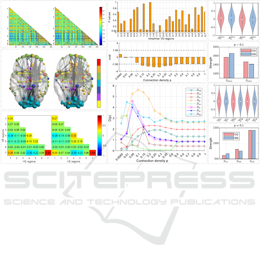
Fig. 2 a shows the heatmaps of group average net-

works for VE-ordered MSNs. In each heatmap, the

value range represented by colors varies from -1 to 1,

and warmer colors indicate higher values. Typically,

MSNs encompass both positive and negative values.

Notably, it appears that there is no discernible visual

distinction between the CG and GG in the heatmaps

of the group average MSNs.

• Comparison of Top 1% Group Brain Net-

works.

Fig. 2 b displays the top 1% (absolute) of group

average brain networks, as visualized using Brain-

Net Viewer (Xia et al., 2013). The seven-colored

nodes represent the grouped VE-Regions, and the

color links denote intra-VE connections, while grey

links denote inter-VE connections. The size of nodes

reﬂects the degree in the network. Top 1% of a brain

network (R = 308) contains [(R −1)R/2] ×1% = 474

connections. Notably, discernible visual differences

exist between the CG and GG average MSNs for

the top 1% of connections: GG shows more intra-

VE connections and fewer inter-VE connections com-

pared to CG.

• Results of Average VE-Region Connections of

Group Brain Networks.

As detailed in Section 2.2.2, we compute the aver-

age VE connection E , for the average brain network

of each group. The results are shown in Figure 2 c.

In the ﬁgure, each cell in the heatmaps represents the

average connection between VE-Regions k and l, de-

noted as E (k,l). The seven diagonal values corre-

spond to the average of connections within each intra-

VE-Region, while the values in the lower triangle rep-

resent the average of connection between each inter-

VE-Region pair. From the visualization, the group

BIOSIGNALS 2025 - 18th International Conference on Bio-inspired Systems and Signal Processing

734

Figure 2: Comparison of CG and GG average brain networks. a. Heatmaps of the CG (left) and GG (right) average networks,

organized by the seven VE-Regions. b. Comparison of the top 1% (absolute) of CG (left) and GG (right) average brain

networks, labeled with seven VE-Regions. c. Average VE-Region connection E of each group average brain network. d. P

values of the Mann–Whitney U test for CG and GG across each VE-Region. e. zval

results of the Mann–Whitney U test

between t

and t

for group average MSNs across different connection densities p. f. Euclidean distance between CG and

GG average networks on each nodal topological feature across different connection densities p. g. Violins for intra-/inter-VE

connections of group average MSNs. h. Strength of intra-VE (S

intra

) and inter-VE (S

inter

) connections for CG and GG at a

connection density of p = 0.1. i. Violins for intra-/inter-hemispheric connections of group average MSNs. j. Strengths of

hemispheric connections, S

, S

and S

, at a connection density of p = 0.1.

average MSNs reveal more pronounced differences

between the CG and GG in the average VE-Region

connections in VE 4-4, 4-6, 5-5, 1-7 and 2-4 (differ-

ences ≥ 0.3). Speciﬁcally, GG exhibits stronger av-

erage connections in VE 4-4 and 4-6, while showing

weaker average connections in VE 5-5, 1-7 and 2-4.

• Signiﬁcant Difference Evaluation Between CG

and GG Across Each VE-Region Connections.

As described in Section 2.2.2, we evaluate the sig-

niﬁcant difference between the connections of A

and A

for each VE-k and VE-l. Figure 2 d provide a

visual representation of P

values resulting from the

Mann–Whitney U test. It is apparent that the group

average MSNs exhibit signiﬁcant differences between

the CG and GG in the VE connections 4-4, 1-7 and 2-

4, with P

< 0.05. Additionally, notable differences

are observed in VE connections 1-2, 1-4 and 4-6,

with P

≳ 0.05. These ﬁndings align closely with the

“Results of average VE-Region connections of group

brain networks,” which also identify pronounced dif-

ferences between CG and GG in VE-Region connec-

tions 4-4, 4-6, 1-7 and 2-4 (differences ≥ 0.3).

3.1.2 Analysis Results of Group Average Brain

Networks Across Different Density

As described in Section 2.2.2, we conducted an anal-

ysis to examine the effects of network density on the

difference between average CG and GG brain net-

works by comparing t

and t

across different con-

nection densities p. Fig. 2 e displays the zval

results

of the Mann–Whitney U test between t

and t

for

group average MSNs across different connection den-

sities p. The zval

values for MSN exceed 1.96 for p

values ranging from 0.15 to 0.4, reaching a maximum

of 2.80 at p = 0.3, indicating signiﬁcantly larger con-

nection values in the CG average MSN compared to

the GG average MSN. Notably, the zval

values stabi-

lize as p ≥ 0.5. This stability arises from the roughly

equal numbers of positive and negative connections in

the MSNs, as observed in Section 3.1.4, with negative

Analyzing Cognitive Patterns in Gifted Children Using MRI and Morphometric Similarity Networks

735

connections being treated as zero. This also explains

the stability observed in the nodal topological feature

analysis when p ≥ 0.5 in the following Section 3.1.3.

3.1.3 Analysis Results of Nodal Topological

Features in Group Networks Across

Various Network Densities

Figure 2 f presents the Euclidean distance D

(p) be-

tween the CG and GG average networks on each

nodal topological feature at different densities p, in-

cluding: D

(teal triangles), D

(red crosses), D

(red circles), D

(orange diamonds), D

(green

dots), D

(purple squares), D

(blue asterisks), D

(cyan stars).

Notably, the trends of D

vs. D

and D

vs. D

exhibit similar patterns as p varies. Additionally, the

values of D

and D

are slightly higher than those of

and D

, respectively. The details are as follows:

• Both D

and D

values start low at very small p

and show a slight increase as p increases, with a

relatively stable trend as p = 0.15 ∼ 0.3.

• Both D

and D

values start low, rise sharply,

peak at p = 0.05, and then decrease rapidly.

• D

values exhibit an early sharp increase, peak-

ing at p = 0.1, followed by a gradual decline.

Despite the decline, they maintain higher values

compared to other features.

• D

values start high, peak early (p = 0.01), and

then decline steadily as density increases, still

maintaining higher values compared to other fea-

tures.

• D

values show an initial peak at lower densities

(p = 0.0065 and p = 0.01), followed by a rapid

decline, stabilizing at very low values.

• D

remain very low values except for a noticeable

increase at p = 0.15.

3.1.4 Results of Intra-/Inter-modular

Connections Based on VE-Regions for

Group Brain Networks

Figure 2 g shows violin plots representing the intra-

VE and inter-VE connections for CG and GG average

MSNs. Each violin includes a white dot representing

the average value. The light red violins correspond

to A

intra

and A

inter

for CG, while the light blue vio-

lins represent A

intra

and A

inter

for GG. The connection

values in the group average MSNs range from −1 to

1. Moreover, the average value of intra-VE connec-

tions is consistently higher than that of inter-VE con-

nections in both CG and GG average MSNs. How-

ever, the differences in intra-VE and inter-VE connec-

tions between CG and GG are minimal in the original

group average MSNs.

Fig. 2 h illustrates the intra-VE connection

strength (S

intra

) and inter-VE connection strength

inter

) for CG and GG at a connection density of

p = 0.1. Both CG and GG exhibit stronger intra-

VE connectivity compared to inter-VE connectivity.

However, GG demonstrates stronger intra-VE con-

nectivity and weaker inter-VE connectivity compared

to CG.

3.1.5 Results of Intra-/Inter-hemispheric

Analysis for Group Average Brain

Networks

Fig. 2 i illustrates the violin plots depicting the intra-

/inter-hemispheric connections of each group average

brain network. The dot in each violin represents the

average value. The light red violins represent the LL,

RR, and LR connections in the average CG brain net-

work, while the light blue violins represent those in

the average GG brain network. It can be observed that

the differences in hemispheric connections between

CG and GG are minimal in the original group average

MSNs.

Fig. 2 j illustrates the hemispheric connection

strengths, S

, S

, and S

, at a connection density

of p = 0.1. The results show that both CG and GG

exhibit stronger right intra-hemispheric connections

than left intra-hemispheric connections, and stronger

inter-hemispheric connections than intra-hemispheric

ones. However, GG shows higher S

, weaker S

and slightly weaker S

compared to CG.

3.2 Results of Individual Cognitive

Analysis for MSNs

As outlined in Section 2.2.3, we analyzed the relation-

ship between cognitive performance and the structural

organization of individual MSNs using Spearman cor-

relation, with the results presented in Fig. 3. As stated

in Section 3.1, stability in MSNs occurs when the con-

nection density p ≥ 0.5. Therefore, our analysis fo-

cuses on connection densities p ≤ 0.6 in this section.

3.2.1 Results of Individual Cognitive Analysis

Based on VE-Regions

As described in 2.2.3, we analyzed the Spearman

correlations between full-scale IQ scores and each

VE-Region connection strength E

(k, l) across dif-

ferent connection densities p. The SCC results

(k, l),C) are shown in Fig. 3 a. Each line corre-

sponds to a different connection density p = 0.0065 ∼

BIOSIGNALS 2025 - 18th International Conference on Bio-inspired Systems and Signal Processing

736

a. b.

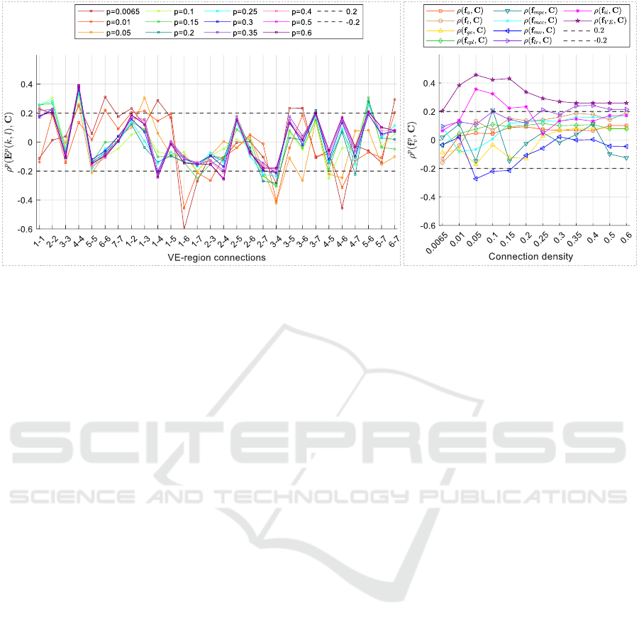
Figure 3: Results of individual cognitive analysis for MSNs. a. SCCs ρ

(k, l),C) between each VE-Region connection

strength E

(k, l) and full-scale IQ scores across different connection densities p. b. SCCs ρ

( f

,C) between various global

topological features (v) of MSNs and full-scale IQ scores (C) across different connection densities p.

0.6. The x-axis represents the various VE-Region

connections, while the y-axis denotes the SCC values.

It can be observed that:

• For lower connection densities (p ≤ 0.05), SCCs

exhibit more pronounced variations and instabil-

ity compared to those observed at higher connec-

tion densities (p ≥ 0.1) for the corresponding VE-

Region connections, particularly in 1-1, 6-6, 1-4,

1-6, 3-6 and 4-6. However, there are higher SCCs

in VE-Region connections of 1-6, 3-4, and 4-6 as

p ≤ 0.05.

• As the connection density p ≥ 0.1, the SCCs for

each VE-Region connection tend to stabilize, with

signiﬁcant positive correlations for VE-Region

connections 1-1, 2-2, 4-4, 3-7, 5-6, 1-2 and 4-

6, signiﬁcant negative correlations for VE-Region

connections 5-5, 1-4, 1-7, 2-4, 2-7, 3-4, 4-5 and

4-7.

3.2.2 Results of Individual Cognitive Analysis

with Global Topological Features

As described in 2.2.3, we analyzed the Spearman cor-

relations between each global topological feature of

brain networks and the full-scale IQ scores across dif-

ferent connection densities p. The results are dis-

played in Fig. 3 b. The x-axis represents different

values of p from 0.0065 to 1, while the y-axis shows

the SCCs for each feature. It can be observed that the

values of ρ

( f

,C) vary with different global topo-

logical features for MSNs:

• IQ is signiﬁcantly positively correlated with the

ratio of intra- to inter-hemispheric connections

( f

) for 0.05 ≤ p ≤ 0.2 (with the highest ρ = 0.36

at p = 0.05), and with the ratio of intra- to inter-

VE connections ( f

V E

) across all p values (with

the highest ρ = 0.46 at p = 0.05). These ﬁnd-

ings suggest that individuals with higher IQ tend

to exhibit stronger intra-hemispheric and intra-

modular connections while displaying weaker

inter-hemispheric and inter-modular connections.

• IQ is signiﬁcantly positively correlated with ra-

tio of left to right intra-hemispheric connec-

tions f

when p = 0.1, indicating stronger left

intra-hemispheric connections in individuals with

higher IQ.

• IQ is signiﬁcantly negatively correlated with

mean versatility f

when 0.05 ≤ p ≤ 0.15, sug-

gesting less versatility in MSNs of individuals

with high cognitive performance.

• Correlations between IQ and mean participation

coefﬁcient f

mpc

exhibit sharp ﬂuctuations as con-

nection density p changes for MSNs.

• There are no signiﬁcant correlations between IQ

and other global topological features, includ-

ing assortativity f

, transitivity f

, global efﬁ-

ciency f

, characteristic path length f

cpl

(aver-

age strength), mean weighted clustering coefﬁ-

cient f

mcc

• Generally, the correlations ρ

( f

,C) tend to

achieve higher values when 0.05 ≤ p ≤ 0.15 in

more cases.

Analyzing Cognitive Patterns in Gifted Children Using MRI and Morphometric Similarity Networks

737

4 DISCUSSION

In this study, we used sMRI data to compute the

MSNs of children with different intelligence levels.

We compared group-level MSNs of CG and GG to

identify key differences and analyzed individual-level

data to link cognitive performance with brain network

structure. The results of our experiments revealed

several important ﬁndings:

• The effects of connection density.

The effects of connection density on brain networks

reveal distinct trends in both group and individual

analyses. (1) Group-level analysis: The signiﬁ-

cant differences between the CG and GG networks

become more pronounced when p = 0.15 ∼ 0.4.

The Euclidean distances between the nodal topolog-

ical features of two groups show high sensitivity to

changes in density when p ≤ 0.05, peaking between

p = 0.05 ∼ 0.25 in most cases. (2) Individual-

level analysis: For VE-Region connections, lower

connection densities (p ≤ 0.05) tend to show more

pronounced variations in correlations with IQ, while

higher densities stabilize these correlations. For

global topological features, higher SCCs are achieved

when p = 0.05 ∼ 0.15. Generally, a connection den-

sity of p = 0.05 ∼ 0.15 is recommended in MSN cog-

nitive analysis for stable and optimal results. Thus,

we chose a connection density of p = 0.1 for group-

level analyses of intra-/inter-modular and intra-/inter-

hemispheric connections.

• The relationship between VE-Region (modu-

lar) connections and cognitive performance.

Both the group and individual analyses reveal that

there are stronger connections in VE 4-4 (secondary

sensory area), 1-2 (motor to association area) and 4-

6 (secondary sensory to limbic area) for individuals

with higher IQ scores. Conversely, weaker connec-

tions in VE 1-7 (motor to insular area), 2-4 (associa-

tion to secondary sensory area) and 1-4 (motor to sec-

ondary sensory area) are observed in individuals with

higher IQ scores. These ﬁndings suggest that higher

cognitive performance is linked not only to enhanced

connectivity in speciﬁc sensory, motor, and limbic ar-

eas but also to a selective reduction in certain modular

connections, potentially contributing to greater neural

efﬁciency.

• Analyses on intra-/inter-modular and intra-

/inter-hemispheric connections

In the group average analysis, both CG and GG

demonstrate stronger intra-VE connections compared

to inter-VE connections, as well as stronger right

intra-hemispheric connections compared to left intra-

hemispheric connections, aligning with (Jiang et al.,

2019). Moreover, both group and individual anal-

yses reveal that individuals with higher IQ tend

to display stronger intra-VE and intra-hemispheric

connections, alongside weaker inter-VE and inter-

hemispheric connections. As stronger MSN con-

nectivity reﬂects greater morphometric similarity, in-

dividuals with higher IQ demonstrate higher mor-

phometric similarity within VE-Regions and hemi-

spheres, alongside greater differentiation between

VE-Regions and between the left and right hemi-

spheres. These ﬁndings suggest a more integrated

intra-hemispheric and intra-VE-Region organization,

which may facilitate more efﬁcient cognitive pro-

cessing (Sol

e-Casals et al., 2019; Santarnecchi et al.,

2015; Krupnik et al., 2021). Additionally, the anal-

ysis shows that a higher ratio of left-to-right intra-

hemispheric connections in MSNs is associated with

enhanced IQ, suggesting that individuals with higher

IQ exhibit a more balanced distribution of connec-

tions between the left and right intra-hemispheric net-

works. Interestingly, this ﬁnding contrasts with (Sol

Casals et al., 2019), which reported stronger right

intra-hemispheric connections for the GG in tradi-

tional SCNs.

• The relationship between topological features

and cognitive performance.

Our analysis reveals signiﬁcant associations between

certain topological features of brain networks and IQ.

(1) Group-level analysis: Sensitivity to connection

density varies across nodal topological features. The

participation coefﬁcient F

, nodal versatility F

, lo-

cal efﬁciency F

and clustering coefﬁcient f

are

sensitive to density variations, and achieve higher

Euclidean distance when p = 0.05 ∼ 0.1. Both the

node degree F

and node strength F

stably achieve

high Euclidean distance as p = 0.15 ∼ 0.3. However,

the node centrality F

and eigenvector centrality F

show little utility for cognitive analysis, as they do

not perform well in distinguishing cognitive groups.

(2) Individual-level analyses: IQ is negatively cor-

related with mean versatility f

at p = 0.05 ∼ 0.1,

contrasting with (Sol

e-Casals et al., 2019), which

found higher mean versatility for the GG in traditional

SCNs. Other features, such as the mean participation

coefﬁcient, show ﬂuctuating correlations across den-

sities are less reliable for MSN cognitive analysis.

This study has some limitations. First, the small

sample size may reduce the generalizability of the

ﬁndings, underscoring the need for larger cohorts in

future research. Second, we neglect the negative value

in MSNs in connection density related analyses, po-

tentially affecting the interpretation of network struc-

tures. Third, while the study focuses on structural

networks, integrating functional imaging data could

BIOSIGNALS 2025 - 18th International Conference on Bio-inspired Systems and Signal Processing

738

provide deeper physiological and cognitive insights.

5 CONCLUSIONS

In this study, we constructed MSNs from sMRI data

to investigate brain network characteristics in chil-

dren with different intelligence levels. Group-level

analyses were performed by comparing the average

MSNs of the CG and GG to identify key differences in

brain network topology. Additionally, we conducted

individual-level analyses to explore the relationship

between cognitive performance and the structural or-

ganization of brain networks.

Our results show that variations in connection

density have a signiﬁcant impact on both global and

nodal topological features, with each exhibiting dis-

tinct trends. A connection density of p = 0.05 ∼ 0.15

is recommended in MSN cognitive analysis for sta-

ble and optimal results. Additionally, gifted indi-

viduals exhibit stronger intra-hemispheric and intra-

modular connectivity, weaker inter-hemispheric and

inter-modular connectivity, a more balanced distri-

bution of left-to-right intra-hemispheric connections,

and lower mean versatility, which may be associ-

ated with more efﬁcient and stable cognitive process-

ing. Moreover, the analyses on anatomical modular-

ity of VE indicate that higher cognitive performance

is linked not only to enhanced connectivity in spe-

ciﬁc modules (such as secondary sensory area, mo-

tor to association area, and secondary sensory to lim-

bic area) but also to a selective reduction in certain

modular connections (such as motor to insular area,

association to secondary sensory area, and motor to

secondary sensory area), potentially contributing to

greater neural efﬁciency. Furthermore, key topolog-

ical features, such as participation coefﬁcient, nodal

versatility, local efﬁciency and clustering coefﬁcient,

are linked to cognitive performance at speciﬁc con-

nection density. However, other features, such as

the mean participation coefﬁcient (showing ﬂuctuat-

ing correlations across densities), assortativity, char-

acteristic path length, and the mean weighted clus-

tering coefﬁcient (showing no signiﬁcant correlations

with IQ), are less reliable for MSN cognitive analysis.

In conclusion, our ﬁndings highlight the effects

of connection density and demonstrate how modu-

lar and hemispheric connectivity, along with speciﬁc

topological features, relate to children’s cognitive per-

formance. These insights pave the way for future re-

search to further explore the neural mechanisms un-

derlying cognitive abilities with brain networks. By

using larger, more diverse samples and longitudinal

designs, future studies could enhance our understand-

ing of how brain network topology evolves with cog-

nitive development and deepen our knowledge of the

neural mechanisms that underpin human intelligence.

ACKNOWLEDGEMENTS

This work was carried out as part of the doctoral pro-

gramm in Experimental Sciences and Technology at

the University of Vic - Central University of Catalo-

nia. F.D. work was partially supported by the National

Natural Science Foundation of China (Key Program)

(No. 11932013), and the Tianjin Science and Tech-

nology Plan Project (No. 22PTZWHZ00040). C.F.C

work was partially supported by grants PICT 2020-

SERIEA-00457 and PIP 112202101 00284CO (Ar-

gentina).

REFERENCES

Blondel, V. D., Guillaume, J.-L., Lambiotte, R., and Lefeb-

vre, E. (2008). Fast unfolding of communities in large

networks. Journal of statistical mechanics: theory

and experiment, 2008(10):P10008.

Brandes, U. (2001). A faster algorithm for between-

ness centrality. Journal of mathematical sociology,

25(2):163–177.

Desikan, R. S., S

egonne, F., Fischl, B., Quinn, B. T., Dick-

erson, B. C., Blacker, D., Buckner, R. L., Dale, A. M.,

Maguire, R. P., Hyman, B. T., et al. (2006). An au-

tomated labeling system for subdividing the human

cerebral cortex on mri scans into gyral based regions

of interest. Neuroimage, 31(3):968–980.

Faskowitz, J., Betzel, R. F., and Sporns, O. (2022). Edges in

brain networks: Contributions to models of structure

and function. Network Neuroscience, 6(1):1–28.

Fischl, B. and Dale, A. M. (2000). Measuring the thickness

of the human cerebral cortex from magnetic resonance

images. Proceedings of the National Academy of Sci-

ences, 97(20):11050–11055.

Genon, S., Eickhoff, S. B., and Kharabian, S. (2022). Link-

ing interindividual variability in brain structure to be-

haviour. Nature Reviews Neuroscience, 23(5):307–

318.

Ghosh, S. S., Kakunoori, S., Augustinack, J., Nieto-

Castanon, A., Kovelman, I., Gaab, N., Christodoulou,

J. A., Triantafyllou, C., Gabrieli, J. D., and Fischl,

B. (2010). Evaluating the validity of volume-based

and surface-based brain image registration for devel-

opmental cognitive neuroscience studies in children 4

to 11 years of age. Neuroimage, 53(1):85–93.

Guimera, R. and Nunes Amaral, L. A. (2005). Functional

cartography of complex metabolic networks. nature,

433(7028):895–900.

Heinsfeld, A. S., Franco, A. R., Craddock, R. C., Buch-

weitz, A., and Meneguzzi, F. (2018). Identiﬁcation of

Analyzing Cognitive Patterns in Gifted Children Using MRI and Morphometric Similarity Networks

739

autism spectrum disorder using deep learning and the

ABIDE dataset. NeuroImage: Clinical, 17:16–23.

Jiang, X., Shen, Y., Yao, J., Zhang, L., Xu, L., Feng, R., Cai,

L., Liu, J., Chen, W., and Wang, J. (2019). Connec-

tome analysis of functional and structural hemispheric

brain networks in major depressive disorder. Transla-

tional psychiatry, 9(1):136.

Kong, X.-z., Liu, Z., Huang, L., Wang, X., Yang, Z., Zhou,

G., Zhen, Z., and Liu, J. (2015). Mapping individual

brain networks using statistical similarity in regional

morphology from mri. PloS one, 10(11):e0141840.

Krupnik, R., Yovel, Y., and Assaf, Y. (2021). Inner

hemispheric and interhemispheric connectivity bal-

ance in the human brain. Journal of Neuroscience,

41(40):8351–8361.

Latora, V. and Marchiori, M. (2001). Efﬁcient behav-

ior of small-world networks. Physical review letters,

87(19):198701.

Li, J., Seidlitz, J., Suckling, J., Fan, F., Ji, G.-J., Meng, Y.,

Yang, S., Wang, K., Qiu, J., Chen, H., et al. (2021).

Cortical structural differences in major depressive dis-

order correlate with cell type-speciﬁc transcriptional

signatures. Nature communications, 12(1):1647.

Li, W., Yang, C., Shi, F., Wu, S., Wang, Q., Nie, Y., and

Zhang, X. (2017). Construction of individual mor-

phological brain networks with multiple morphomet-

ric features. Frontiers in Neuroanatomy, 11:34.

Lo, C.-Y. Z., He, Y., and Lin, C.-P. (2011). Graph theoret-

ical analysis of human brain structural networks. Re-

views in the Neurosciences, 22(5):551–563.

Newman, M. (2010). Networks: An Introduction. Oxford

University Press.

Newman, M. E. (2002). Assortative mixing in networks.

Physical review letters, 89(20):208701.

Onnela, J.-P., Saram

aki, J., Kert

esz, J., and Kaski, K.

(2005). Intensity and coherence of motifs in weighted

complex networks. Physical Review E—Statistical,

Nonlinear, and Soft Matter Physics, 71(6):065103.

Park, H.-J. and Friston, K. (2013). Structural and functional

brain networks: from connections to cognition. Sci-

ence, 342(6158):1238411.

Rubinov, M. and Sporns, O. (2010). Complex network mea-

sures of brain connectivity: uses and interpretations.

Neuroimage, 52(3):1059–1069.

Santarnecchi, E., Tatti, E., Rossi, S., Serino, V., and Rossi,

A. (2015). Intelligence-related differences in the

asymmetry of spontaneous cerebral activity. Human

brain mapping, 36(9):3586–3602.

Sebenius, I., Seidlitz, J., Warrier, V., Bethlehem, R. A.,

Alexander-Bloch, A., Mallard, T. T., Garcia, R. R.,

Bullmore, E. T., and Morgan, S. E. (2023). Robust

estimation of cortical similarity networks from brain

mri. Nature Neuroscience, 26(8):1461–1471.

Seidlitz, J., V

sa, F., Shinn, M., Romero-Garcia, R.,

Whitaker, K. J., V

ertes, P. E., Wagstyl, K., Reardon,

P. K., Clasen, L., Liu, S., et al. (2018). Morphometric

similarity networks detect microscale cortical organi-

zation and predict inter-individual cognitive variation.

Neuron, 97(1):231–247.

Shinn, M., Romero-Garcia, R., Seidlitz, J., V

sa, F.,

ertes, P. E., and Bullmore, E. (2017). Versatility of

nodal afﬁliation to communities. Scientiﬁc Reports,

7(1):4273.

Sol

e-Casals, J., Serra-Grabulosa, J. M., Romero-Garcia,

R., Vilaseca, G., Adan, A., Vilar

o, N., Bargall

o, N.,

and Bullmore, E. T. (2019). Structural brain net-

work of gifted children has a more integrated and

versatile topology. Brain Structure and Function,

224(7):2373–2383.

Sun, K., Chen, G., Liu, C., Chu, Z., Huang, L., Li, Z.,

Zhong, S., Ye, X., Zhang, Y., Jia, Y., et al. (2024a). A

novel msn-ii feature extracted from t1-weighted mri

for discriminating between bd patients and mdd pa-

tients. Journal of Affective Disorders.

Sun, Y., Chen, P., Liu, Y., and Zhao, K. (2024b). Macroscale

brain structural network coupling is related to ad pro-

gression. In 2024 IEEE International Symposium on

Biomedical Imaging (ISBI), pages 1–4. IEEE.

Sun, Y., Lee, R., Chen, Y., Collinson, S., Thakor, N., Bez-

erianos, A., and Sim, K. (2015). Progressive gen-

der differences of structural brain networks in healthy

adults: a longitudinal, diffusion tensor imaging study.

PloS one, 10(3):e0118857.

Van Wijk, B. C., Stam, C. J., and Daffertshofer, A. (2010).

Comparing brain networks of different size and con-

nectivity density using graph theory. PloS one,

5(10):e13701.

sa, F., Seidlitz, J., Romero-Garcia, R., Whitaker, K. J.,

Rosenthal, G., V

ertes, P. E., Shinn, M., Alexander-

Bloch, A., Fonagy, P., Dolan, R. J., et al. (2018). Ado-

lescent tuning of association cortex in human struc-

tural brain networks. Cerebral Cortex, 28(1):281–

294.

ertes, P. E., Rittman, T., Whitaker, K. J., Romero-Garcia,

R., V

sa, F., Kitzbichler, M. G., Wagstyl, K., Fonagy,

P., Dolan, R. J., Jones, P. B., et al. (2016). Gene tran-

scription proﬁles associated with inter-modular hubs

and connection distance in human functional magnetic

resonance imaging networks. Philosophical Trans-

actions of the Royal Society B: Biological Sciences,

371(1705):20150362.

Von Economo, C. (1929). The cytoarchitectonics of the hu-

man cerebral cortex. H. Milford Oxford University

Press.

Watts, D. J. and Strogatz, S. H. (1998). Collective dynam-

ics of ‘small-world’networks. nature, 393(6684):440–

442.

Xia, M., Wang, J., and He, Y. (2013). Brainnet viewer:

a network visualization tool for human brain connec-

tomics. PloS one, 8(7):e68910.

Yu, K., Wang, X., Li, Q., Zhang, X., Li, X., and Li, S.

(2018). Individual morphological brain network con-

struction based on multivariate euclidean distances be-

tween brain regions. Frontiers in human neuroscience,

12:204.

Zhang, J., Feng, F., Han, T., Duan, F., Sun, Z., Caiafa, C. F.,

and Sol

e-Casals, J. (2021). A hybrid method to select

morphometric features using tensor completion and f-

score rank for gifted children identiﬁcation. Science

China Technological Sciences, 64(9):1863–1871.

BIOSIGNALS 2025 - 18th International Conference on Bio-inspired Systems and Signal Processing

740