A Stochastic Location-Routing Problem for the Optimal Placement of

Lockers

Guido Barbieri

, Annarita De Maio

2 a

, Roberto Musmanno

1 b

and Sara Stoia

2 c

Department of Mechanical, Energy and Management Engineering, University of Calabria, Italy

Department of Economics, Statistics and Finance ”Giovanni Anania”, University of Calabria, Italy

Keywords:

Stochastic Location-Routing Problem, Parcel Lockers, Last-Mile Delivery, Vehicle Routing, Uncertainty,

Two-Stage Stochastic Programming.

Abstract:

This paper presents a Stochastic Location-Routing Problem aimed at optimizing the placement of parcel lock-

ers in last-mile delivery. The model integrates locker location decisions with vehicle routing, taking into

account customer preferences for home delivery or locker collection. It considers multiple scenarios of ser-

vice requests to address the uncertainty in customer behavior. The problem is formulated as a two-stage

stochastic program, where the ﬁrst stage determines which lockers to activate, and the second stage optimizes

vehicle routes based on the service preferences for each scenario. Computational experiments are based on a

test problem used to validate the model’s effectiveness. Proposed future extensions include integrating multi-

period planning, introducing capacity constraints for both vehicles and lockers, enabling dynamic activation of

lockers, and optimizing the algorithm for multi-core architectures to enhance computational efﬁciency. These

advancements aim to enhance the model’s applicability and scalability in tackling complex logistics challenges

under uncertainty.

1 INTRODUCTION

In recent years, the rapid growth of online shopping

across various industries has created ongoing chal-

lenges for companies handling the delivery of high

volumes of parcels to increasingly demanding cus-

tomers.

In this scenario, optimizing last-mile delivery, par-

ticularly in densely populated urban areas, has be-

come essential for both business efﬁciency and envi-

ronmental sustainability. To reduce delivery costs and

minimize the ecological impact of last-mile logistics,

innovative strategies are being introduced, with one

prominent solution being the implementation of elec-

tronic, self-service lockers, placed in accessible pub-

lic locations and serving as convenient pick-up points

for online orders (Grabenschweiger et al., 2021).

The introduction of lockers offers beneﬁts for both

companies and customers. Customers gain the ﬂexi-

bility to customize their delivery experience by choos-

ing between home delivery or secure locker collection

https://orcid.org/0000-0002-4650-3362

https://orcid.org/0000-0002-8852-6933

https://orcid.org/0009-0001-1955-501X

at a convenient time. For companies, lockers enable

the consolidation of deliveries to fewer locations, re-

ducing inefﬁciencies such as missed deliveries when

customers are unavailable. Furthermore, placing par-

cel lockers in urban areas increases delivery capacity

without the need to expand the workforce, which also

helps to reduce the environmental footprint (Oren-

stein et al., 2019).

Today, various types of lockers exist. Schwerd-

feger and Boysen (2022) distinguishes between sta-

tionary and mobile infrastructures. Stationary lock-

ers, which are the most common, remain ﬁxed after

installation, whereas Mobile Parcel Lockers (MPLs)

can be relocated as needed.

Determining the optimal location for installing a

parcel locker and planning deliveries at an operational

level are both complex and interdependent decisions.

It is important to note that the choice between deliv-

ery to a locker or directly to the customer’s home is

made by the customer, not the service provider. This

introduces a level of uncertainty that must be factored

into the decision-making process (Lai et al., 2022;

Rossolov, 2023).

Under this perspective, this work proposes a

stochastic model that integrates locker location and

Barbieri, G., De Maio, A., Musmanno, R. and Stoia, S.

A Stochastic Location-Routing Problem for the Optimal Placement of Lockers.

DOI: 10.5220/0013170500003893

Paper published under CC license (CC BY-NC-ND 4.0)

In Proceedings of the 14th International Conference on Operations Research and Enterprise Systems (ICORES 2025), pages 123-132

ISBN: 978-989-758-732-0; ISSN: 2184-4372

123

vehicle routing costs, taking into account customer

time windows and variability in service type selection

to optimize operations comprehensively.

The problem can be modeled as a Stochastic

Location-Routing Problem (SLRP). The determinis-

tic version of the problem (LRP) has been discussed

in the literature for a long time. The earliest ex-

amples refer to Von Boventer (1961) and Maranzana

(1964). However, LRP has gained substantial pop-

ularity in the scientiﬁc community only recently, as

demonstrated in the surveys of Drexl and Schneider

(2015) and Mara et al. (2021).

Indeed, the location of a logistics node, if de-

termined without considering the impact on the re-

sulting routes, may lead to sub-optimal decisions in

terms of overall logistics costs. An integrated ap-

proach that accounts for both node location and route

optimization is therefore essential to minimize oper-

ational costs and enhance the efﬁciency of the distri-

bution network. This problem encompasses two NP-

hard problems, making LRP itself an NP-hard prob-

lem (Nagy and Salhi, 2007).

This class of problems has been used in the litera-

ture to model applications in different contexts. Some

recent examples in a deterministic setting are the fol-

lowing.

In Veenstra et al. (2021), lockers are used for phar-

maceutical deliveries without considering time win-

dows or locker capacities. Conversely, Liu et al.

(2021) apply lockers in a grocery distribution con-

text, taking into account both time windows and ca-

pacity constraints for lockers and depots. Wang et al.

(2022a) propose an LRP model for last-mile distribu-

tion, where customers can be served either by small

electric vehicles or through lockers, while consider-

ing the battery levels of the vehicles. Liu et al. (2015)

extend the LRP into the Location-Inventory-Routing

Problem, formulating a model that locates logistic

nodes for both parcel distribution and returns collec-

tion. The model also incorporates inventory deci-

sions, aiming to minimize the costs of location, trans-

portation, inventory, and parcel returns.

In the literature, the concept of lockers can be ex-

tended to include similar options, such as Collection-

and-Delivery Points (CDPs). These represent generic

logistic nodes for parcel collection and delivery,

which, unlike lockers, can include stores and private

postal services that offer such services during their

operating hours. Rautela et al. (2022) formulates a de-

terministic LRP model to locate CDPs within a com-

plex logistics network.

A paper addressing a problem similar to the one

under analysis is presented by Grabenschweiger and

Dorner (2022). They examine a multi-period LRP

for locker location, taking time windows into ac-

count. However, their model handles customer-to-

locker assignments without considering uncertainty in

customer service type selection. Liu et al. (2023b) ex-

plore a special case of LRP, focusing on the daily relo-

cation of MPLs to minimize overall operational costs

and enhance customer accessibility.

Although incorporating uncertain data makes

models more realistic, only a small portion of the

studies on LRP consider stochastic data, as high-

lighted by Mara et al. (2021). An example of a SLRP

is presented by Aghalari et al. (2023), who formu-

late an SLRP model for locating charging stations for

electric vehicles used in distribution. The model ac-

counts for uncertainty in customer demand and envi-

ronmental factors, which directly affect battery efﬁ-

ciency. The objective is to minimize location costs

and the expected routing costs.

Other applications of SLRPs can be found in hu-

manitarian logistics, as discussed by de Veluz et al.

(2023), which focuses on the location of distribution

and evacuation centers while considering various dis-

aster scenarios. The model aims to minimize costs,

the number of vehicles used, and travel times.

This study contributes to the body of knowledge

on SLRPs as it is the ﬁrst in the literature to address

locker location while considering customer time win-

dows, uncertainty in customer service selection, and

multi-period planning.

The remainder of the paper is organized as fol-

lows. In Section 2 we report a formal discussion of

the SLRP and the corresponding mathematical formu-

lation. In Section 3 we describe the solution method

proposed. In Section 4, we discuss the results of our

computational experiments. Conclusions and future

developments follow in Section 5.

2 MATHEMATICAL

FORMULATION

We consider a complete directed graph G = (N,A),

where N represents the set of nodes. Node 0 specif-

ically corresponds to the depot from which all routes

must start. Additionally, let the sets C and L be sub-

sets of N, where C represents the set of customers

(with each customer indexed by c), and L repre-

sents the set of potential sites for locker placement

(with each locker site indexed by l). Thus, we have

N = 0 ∪ C ∪ L. A represents the set of arcs, where

each arc (i, j) corresponds to the fastest path from

node i to node j in G.

For each customer c ∈ C, let π

represent the prob-

ability of serving the customer at their home. Conse-

ICORES 2025 - 14th International Conference on Operations Research and Enterprise Systems

124

quently, 1 − π

corresponds to the probability that the

customer will opt to collect their delivery from the

nearest locker. These probabilities can be estimated

using historical data on service preferences from the

previous purchases of each customer.

A binary constant g

is associated with each cus-

tomer, where g

= 1 if the customer is served at home

and g

= 0 if the service is provided through a locker.

This allows the formulation of a stochastic program-

ming problem to handle uncertainty by introducing a

set S of scenarios. Each scenario s ∈ S represents a

possible service conﬁguration for all customers, de-

ﬁned by a vector of |C| binary elements, with an asso-

ciated probability

(s)

∏

c∈C

(s)

where p

(s)

= π

if g

= 1 in scenario s, and p

(s)

1 − π

if g

= 0.

The total number of scenarios is therefore equal to

|C|

The stochastic programming problem is structured

as a two-stage model. In the ﬁrst stage, decisions

are made regarding the placement of lockers, which

must be ﬁnalized before customers select their pre-

ferred service option (either home delivery or locker

collection). The second stage involves making rout-

ing decisions, which occur after customers have cho-

sen their service type.

The SLRP, in its most general form, can be multi-

period, with T representing the set of time periods that

deﬁne the planning horizon.

The input parameters of the problem are as fol-

lows:

• n: number of lockers to be activated (n ≤ |L|);

• d

i j

, (i, j) ∈ A: distance associated with arc (i, j);

• t

i j

, (i, j) ∈ A: travel time along arc (i, j);

• γ

i j

, (i, j) ∈ A: transportation cost along arc (i, j);

• δ

, c ∈ C, l ∈ L: transportation penalty cost in-

curred when a customer c is served by a locker l

located at a distance d

> ρ, where ρ is a thresh-

old set by the decision-maker. Speciﬁcally, ρ cor-

responds to the maximum distance a customer is

willing to travel to a locker. The penalty cost

= 0 if d

≤ ρ, and δ

= r(d

− ρ) otherwise,

where r is a unit penalty cost;

• a

, c ∈ C, t ∈ T : binary coefﬁcient equal to 1 if

customer c must be served in time period t, 0 oth-

erwise;

• g

(s)

, c ∈ C, s ∈ S: binary coefﬁcient indicating

whether, in scenario s, customer c is served at

home (g

(s)

= 1) or via a locker (g

(s)

= 0);

• e

, i ∈ N: earliest time at which service can start

at node i;

• l

, i ∈ N: latest time by which service must start at

node i;

• τ

, i ∈ N: service time at node i;

• f

, l ∈ L : activation cost of locker l;

• p

(s)

, s ∈ S : probability associated with scenario s;

• k: number of available vehicles;

• M: arbitrarily large constant.

The decision variables are the following.

First-stage variables:

• w

, l ∈ L: binary variable indicating whether a

locker is opened in site l.

Recourse variables:

• x

(s)

i jt

, (i, j) ∈ A, t ∈ T, s ∈ S : binary variable equal

to 1 if arc (i, j) is traversed by a vehicle during

time period t in scenario s, 0 otherwise;

• y

(s)

clt

, c ∈ C, l ∈ L, t ∈ T , s ∈ S: binary variable

equal to 1 if customer c is assigned to locker l

and served during time period t in scenario s, 0

otherwise;

• z

(s)

, c ∈ C, t ∈ T , s ∈ S: binary variable equal to 1

if customer c is served at home during time period

t in scenario s, 0 otherwise;

• v

(s)

, i ∈ N, t ∈ T, s ∈ S: non-negative continuous

variable representing the start time of the visit to

node i during time period t in scenario s.

The objective of the SLRP is to minimize the total

cost, which is inﬂuenced by three components:

• transportation costs associated with vehicle routes

that visit both home customers and lockers:

(s)

∑

(i, j)∈A

∑

t∈T

i j

(s)

i jt

;

• penalty costs related to the service level, reﬂecting

limitations on assigning customers to lockers that

are too distant:

(s)

∑

c∈C

∑

l∈L

∑

t∈T

(s)

clt

;

• locker activation costs:

∑

l∈L

Note that both the transportation costs and penalty

costs depend on recourse decisions and thus vary

across scenarios s ∈ S, whereas the locker activation

costs are invariant across scenarios, as they are asso-

ciated with the ﬁrst-stage decisions.

A Stochastic Location-Routing Problem for the Optimal Placement of Lockers

125

The formulation of the two-stage model is the fol-

lowing:

min

∑

s∈S

(s)

+ z

(s)

) + z

(1)

subject to

∑

j∈N\{i}

(s)

i jt

≤ 1, ∀ i ∈ N \ {0},∀ t ∈ T,∀ s ∈ S (2)

∑

j∈N\{0}

(s)

0 jt

≤ k, ∀ t ∈ T,∀ s ∈ S (3)

∑

j∈N\{i}

(s)

i jt

∑

j∈N\{i}

(s)

jit

, ∀ i ∈ N, ∀ t ∈ T,∀ s ∈ S (4)

(s)

clt

≤

∑

j∈N\{l}

(s)

l jt

, ∀ c ∈ C,∀ l ∈ L, ∀ t ∈ T,∀ s ∈ S (5)

(s)

≤

∑

j∈N\{c}

(s)

c jt

, ∀ c ∈ C, ∀ t ∈ T, ∀ s ∈ S (6)

∑

j∈N\{l}

(s)

l jt

≤ w

, ∀ l ∈ L,∀ t ∈ T, ∀ s ∈ S (7)

∑

l∈L

= n (8)

∑

l∈L

(1 − g

(s)

) y

(s)

clt

+ g

(s)

= a

, ∀ c ∈ C, ∀ t ∈ T,∀ s ∈ S (9)

(s)

+ τ

i j

− M (1 − x

(s)

i jt

) ≤ v

(s)

, ∀ i ∈ N,

∀ j ∈ N \ {0},∀ t ∈ T, ∀ s ∈ S

(10)

(s)

+ τ

≤ l

, ∀ i ∈ N,∀ t ∈ T, ∀ s ∈ S (11)

(s)

≤ l

∑

j∈N\{i}

(s)

i jt

, ∀ i ∈ N \ {0},∀ t ∈ T,∀ s ∈ S (12)

(s)

≥ e

∑

j∈N\{i}

(s)

i jt

, ∀ i ∈ N, ∀ t ∈ T, ∀ s ∈ S (13)

(s)

i jt

∈ {0, 1}, ∀ (i, j) ∈ A,∀ t ∈ T,∀ s ∈ S (14)

(s)

clt

∈ {0,1}, ∀ c ∈ C,∀ l ∈ L, ∀ t ∈ T, ∀ s ∈ S (15)

(s)

∈ {0,1}, ∀ c ∈ C,∀ t ∈ T,∀ s ∈ S (16)

∈ {0,1}, ∀ l ∈ L (17)

(s)

≥ 0, ∀ i ∈ N,∀ t ∈ T,∀ s ∈ S. (18)

In the objective function (1), the transportation

and penalty costs are weighted according to the prob-

abilities of the scenarios. Constraints (2) ensure that

each node (except the depot) is visited at most once

per time period in each scenario. Constraints (3) re-

strict the number of routes to the number of avail-

able vehicles in each time period and for each sce-

nario. Equations (4) represent the ﬂow balance con-

straints for each node, in every time period and for

each scenario. Constraints (5) link the variables y

(s)

clt

to the variables x

(s)

l jt

, ensuring that for each scenario

s, if a customer c is served by locker l in time period

t, the node corresponding to that locker must be vis-

ited during that time period. Constraints (6) link the

variables z

(s)

to the variables x

(s)

c jt

, ensuring that for

each scenario s, if a customer c is served at home in

time period t, the node corresponding to that customer

must be visited during that time period. Constraints

(7) ensure that for each time period and scenario, if

a locker is not opened, its corresponding node can-

not be visited. Constraint (8) imposes the required

number of lockers to be activated. Constraints (9) en-

sure that each customer is served either at home or

through a locker, depending on the scenario s. Con-

straints (10)−(11) ensure temporal continuity of ser-

vice and prevent the formation of sub-tours within the

routes. Additionally, constraints (11) ensure that the

time window for the depot is respected in every time

period and scenario. Constraints (12)−(13) impose

the satisfaction of time windows for each node, time

period, and scenario. Finally, constraints (14)−(18)

deﬁne the nature (binary or continuous) of the deci-

sion variables.

For simplicity, the remainder of this paper focuses

on a single time period within the planning horizon,

assuming that the available vehicle ﬂeet is sufﬁciently

large to meet all customer demand.

3 SOLUTION METHOD

When solving the SLRP for locker location to opti-

mality, it is theoretically possible to approach the so-

lution by inspection, at least in principle. Speciﬁcally,

all possible



|L|



combinations of locker activations

from the set of potential sites are considered and ex-

amined individually. By deﬁning the values of the

location variables w

for each combination, their ef-

fect on second-stage decisions can be evaluated by

solving a Vehicle Routing Problem with Time Win-

dows (VRP-TW) for each scenario. The nodes to be

visited in each VRP-TW include the activated lockers

and the customers who, in the corresponding scenario,

ICORES 2025 - 14th International Conference on Operations Research and Enterprise Systems

126

are scheduled for home delivery.

After solving the VRP-TW for each scenario s ∈ S,

the total solution cost for the SLRP can be calculated

using equation (1).

The pseudo-code of the proposed procedure for

solving the SLRP for each choice of n lockers to acti-

vate is presented below.

Algorithm 1: Procedure SLRP. (L, z).

begin

// L is the set of n lockers to

be activated

// z is the total cost of the

SLRP

1 z

∑

l∈L

;

2 z = z

;

3 for s = 1 to |S| do

4 Determine the list C

(s)

of customers

who, according to scenario s, request

home delivery;

// C

(s)

is the list of

customers served via lockers

5 C

(s)

= C \C

(s)

6 for c = 1 to |C

(s)

| do

7 Assign c to the nearest locker

l ∈ L;

8 Determine the penalty δ

;

9 end

10 z

(s)

∑

c∈C

(s)

∑

l∈L

;

// Update z

11 z := z + p

(s)

;

// Define the set N of nodes

for which the VRP-TW will be

solved

12 N = 0 ∪C

(s)

∪ L;

13 Solve the VRP-TW on the complete

directed graph induced by N;

// z

(s)

is the cost of the

VRP-TW

// Update z

14 z := z + p

(s)

;

15 end

16 return z;

end

The time complexity of the entire algorithm

grows exponentially with the problem size, making it

quickly impractical even for moderately sized inputs,

as the execution time increases rapidly.

To keep execution times within acceptable limits,

three approaches can be applied simultaneously: 1)

reducing the number of conﬁgurations of n lockers

to test among the |L| possible choices (this reduces

the number of calls of the SLRP procedure); 2) re-

ducing the number of scenarios in the for loop 3−15

of the SLRP procedure; and 3) heuristically solving

the VRP-TW for each scenario (code line 13 of the

SLRP procedure). These three proposed approaches

are brieﬂy outlined below.

3.1 Reduction of the Number of Locker

Conﬁgurations

For limiting the number of locker conﬁgurations to be

tested, geographical criteria are widely used and pro-

posed in literature to optimize placement and enhance

efﬁciency (Lagorio and Pinto (2020), Sawik (2024)

and Wang et al. (2022b)). Here are the two relevant

approaches:

• optimal geographical coverage: lockers should

be strategically placed to ensure even distribution

across the service area, minimizing coverage gaps

and guaranteeing accessibility in all key locations;

• proximity between lockers: it is possible to avoid

placing lockers too close to one another, prevent-

ing redundancy and enhancing the overall efﬁ-

ciency of the locker network.

3.2 Reduction of the Number of

Scenarios

As observed in Section 2, the number of scenar-

ios grows exponentially with the number of cus-

tomers. To give an idea, considering 30 customers

would result in a number of scenarios equal to 2

1,073,741,824. This implies that only a representative

subset S of all possible scenarios may be considered.

To reduce the number of scenarios, the following

approach is proposed. First, the most likely scenario

∗

is considered. The probability p

∗

)

of this scenario

is equal to the product of the probabilities associated

with each individual customer corresponding to the

most probable choice:

∗

)

∏

c∈C

max{π

;1 − π

Then, |S| scenarios are randomly generated, en-

suring that the overall probability (given by the sum

of the scenario probabilities) is greater than or equal

A Stochastic Location-Routing Problem for the Optimal Placement of Lockers

127

Algorithm 2: Procedure Scenario Generation.

begin

// Σ is a binary matrix of

scenarios, with size |S| × |C|

1 Randomly generate Σ;

2 Determine the cumulative probability

(Σ)

|S|

∑

s=1

(s)

associated with the

scenarios in Σ;

3 while p

(Σ)

< p

∗

)

4 Randomly select an entry (s,c) of Σ;

5 if p

(s)

< max{π

;1 − π

} then

6 p

(s)

= max{π

;1 − π

};

7 Modify scenario s in Σ

accordingly;

8 Update p

(Σ)

;

9 end

10 end

end

to p

∗

)

. The proposed procedure is illustrated in the

sequel.

Finally, to ensure consistent comparison between

solutions derived from different scenario subsets, we

normalize the associated probabilities so that the over-

all probability across all scenarios s ∈ S equals one.

This is achieved by replacing each value of p

(s)

for all

s ∈

S at the end of the Scenario Generation proce-

dure with the ratio p

(s)

(Σ)

3.3 Heuristic Approaches for the

VRP-TW

Several methods can be applied to generate feasible

vehicle routes while respecting time windows con-

straints. As reported in Liu et al. (2023a), most

of these methods fall into three categories: exact,

heuristic, and metaheuristic approaches. Heuristic

and metaheuristic methods, starting with Solomon’s

constructive heuristics (Solomon, 1987), are widely

used in the literature due to their ability to efﬁciently

solve large-scale problems.

Exact methods are also worth mentioning, though

they are generally capable of optimally solving only

small to medium-sized problems (Desaulniers et al.,

2005) . Among them, the column generation method

stands out, as it can be adapted for the VRP-TW

to generate sub-optimal solutions within acceptable

computational times (Kallehauge et al., 2005).

4 COMPUTATIONAL

EXPERIMENTS

The solution method described in Section 3 was tested

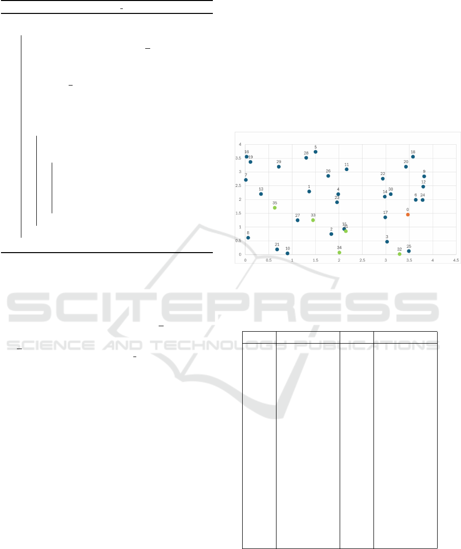
on a problem consisting of |N| = 36 nodes, where

their spatial distribution on the plane was randomly

generated (see Figure 1). Table 1 presents the Carte-

sian coordinates of the nodes. Node 0 represents the

depot, nodes 1 to 30 correspond to the customers, and

nodes 31 to 35 indicate the potential sites for locker

locations.

Figure 1: Spatial distribution of the nodes of the test prob-

lem.

Table 1: Cartesian coordinates (in kilometres) of the nodes

of the test problem.

Node Coordinates Node Coordinates

0 (3.47, 1.46) 1 (1.36, 2.29)

2 (1.84, 0.75) 3 (3.03, 0.47)

4 (1.98, 2.20) 5 (1.50, 3.73)

6 (3.64, 1.99) 7 (0.02, 2.71)

8 (0.06, 0.61) 9 (3.82, 2.84)

10 (0.90, 0.05) 11 (2.17, 3.10)

12 (3.80, 2.47) 13 (0.34, 2.20)

14 (2.98, 2.10) 15 (2.11, 0.93)

16 (0.03, 3.55) 17 (2.99, 1.35)

18 (3.58, 3.55) 19 (0.11, 3.36)

20 (3.43, 3.19) 21 (0.68, 0.19)

22 (2.94, 2.76) 23 (1.96, 1.90)

24 (3.79, 1.98) 25 (3.49, 0.13)

26 (1.77, 2.86) 27 (1.12, 1.25)

28 (1.30, 3.51) 29 (0.72, 3.19)

30 (3.11, 2.19) 31 (2.15, 0.85)

32 (3.29, 0.02) 33 (1.45, 1.25)

34 (2.01, 0.08) 35 (0.63, 1.70)

The distances between nodes (in kilometers) are

Euclidean, thereby ensuring the triangular inequality

property. Table 2 presents the time windows and ser-

vice times for each node, expressed in hours. The

time windows are set starting from 00:00.

ICORES 2025 - 14th International Conference on Operations Research and Enterprise Systems

128

The transportation cost γ

i j

for each arc (i, j ) ∈ A

is deﬁned as:

i j

= 1.0 × d

i j

where 1.0 represents the unit transportation cost (in

e/km). The unit penalty cost is set to 0.60 e/km. The

ﬁxed opening cost of a locker is assumed to be iden-

tical for each potential site ( f

= f ,∀ l ∈ L). As a

result, the cost z

in the objective function (1) is the

same for every locker conﬁguration tested (z

= f n)

and is therefore omitted. The ﬂeet consists of k = 4

vehicles.

Table 2: Time windows (e

, l

) and service times (τ

) for

each node i ∈ N.

Node i e

0 0 24 0.0 1 10 15 0.1

2 9 13 0.1 3 14 17 0.1

4 12 16 0.1 5 8 15 0.1

6 9 11 0.1 7 10 14 0.1

8 16 18 0.1 9 10 13 0.1

10 11 15 0.1 11 12 17 0.1

12 15 16 0.1 13 10 13 0.1

14 10 14 0.1 15 8 10 0.1

16 9 13 0.1 17 15 17 0.1

18 14 16 0.1 19 12 14 0.1

20 13 16 0.1 21 10 11 0.1

22 9 12 0.1 23 14 16 0.1

24 12 13 0.1 25 14 16 0.1

26 12 15 0.1 27 10 11 0.1

28 12 14 0.1 29 8 9 0.1

30 15 16 0.1 31 9 18 0.3

32 9 18 0.3 33 9 18 0.3

34 9 18 0.3 35 9 18 0.3

The probabilities of home service for the 30 cus-

tomers are presented in Table 3.

Consequently, the most likely scenario s

∗

, corre-

sponding to the 30 binary entries reported in Table 4,

has a probability p

∗

)

= 0.000354352.

We consider the case where two lockers are to be

activated out of the ﬁve potential sites. In this case,

the SLRP can be solved for each possible conﬁgura-

tion of locker activation, as the number is small, being





2!×3!

= 10.

Regarding the scenarios, computational experi-

ments were conducted considering two situations: 1)

only scenario s

∗

, corresponding to the most likely ser-

vice conﬁguration, for which the probability p

∗

)

set to one; and 2) using a set S of 30 representative

scenarios, deemed sufﬁcient to capture the stochas-

tic nature of the problem. These scenarios were

generated using the Scenario Generation procedure,

which produced the binary matrix Σ of size 30×30,

with a cumulative probability p

= 0.000381808. The

Table 3: Probabilities of service at home for the 30 cus-

tomers.

Customer Probability Customer Probability

) (c) (π

)

1 0.0449 2 0.9441

3 0.1970 4 0.6387

5 0.0678 6 0.3687

7 0.8344 8 0.8841

9 0.4342 10 0.9260

11 0.2256 12 0.0765

13 0.0425 14 0.7687

15 0.4447 16 0.7207

17 0.6687 18 0.8906

19 0.3913 20 0.2988

21 0.6518 22 0.9872

23 0.2420 24 0.9467

25 0.6288 26 0.6725

27 0.7480 28 0.0616

29 0.5331 30 0.8611

Table 4: Home delivery (1) or service via locker (0) for the

30 customers in the most likely scenario s

∗

Customer (c) g

∗

)

Customer (c) g

∗

)

1 0 2 1

3 0 4 1

5 0 6 0

7 1 8 1

9 0 10 1

11 0 12 0

13 0 14 1

15 0 16 1

17 1 18 1

19 0 20 0

21 1 22 1

23 0 24 1

25 1 26 1

27 1 28 0

29 1 30 1

probabilities of each scenario in S were then normal-

ized so that

∑

s∈S

(s)

= 1.

It is worth emphasizing that solving the SLRP by

considering only the most likely scenario effectively

transforms it into a deterministic problem, where ser-

vice decisions are made under the assumption that

each customer will always choose their most pre-

ferred service.

From this perspective, the ”single scenario” model

does not account for uncertainty and is therefore re-

ferred to as the deterministic case hereafter.

The entire algorithm was implemented in Python

3 using the Visual Studio Code IDE. To solve the

VRP-TW, we used the VRPy library, a package de-

A Stochastic Location-Routing Problem for the Optimal Placement of Lockers

129

Figure 2: Costs obtained for each the ten tested locker conﬁgurations, both in the deterministic case (in blue) and the stochastic

case (in red).

Table 5: Pair of activated lockers, transportation cost (z

penalty cost (z

), and total cost (z) for each of the ten locker

conﬁgurations in the deterministic case.

Conﬁguration L z

1 31, 32 17.32 10.77 28.09

2 31, 33 17.75 8.69 26.44

3 31, 34 17.34 10.74 28.08

4 31, 35 20.05 7.57 27.62

5 32, 33 20.57 8.88 29.45

6 32, 34 18.05 14.09 32.14

7 32, 35 20.83 9.21 30.04

8 33, 34 18.52 9.52 28.04

9 33, 35 20.31 8.66 28.97

10 34, 35 20.86 9.42 30.28

signed for solving various vehicle routing problems

through a column generation approach (Montagn

et al., 2020). In this method, routes (or columns)

are generated by solving a pricing problem and then

passed to a master problem, which selects the best

routes from a pool such that each vertex (except the

depot) is served exactly once. It is important to note

that VRPy does not necessarily return an optimal so-

lution, but feasibility is guaranteed.

The results are summarized in Tables 5 and 6 for

the deterministic and stochastic cases of the problem,

respectively. The tables are organized as follows:

column Conﬁguration enumerates the ten conﬁgu-

Table 6: Transportation costs (z

), penalty costs (z

), and

total costs (z) for the ten activated locker conﬁgurations in

the stochastic case.

Conﬁguration L z

1 31, 32 18.89 10.95 29.84

2 31, 33 19.27 8.81 28.08

3 31, 34 18.77 10.85 29.62

4 31, 35 20.23 7.63 27.86

5 32, 33 19.62 9.14 28.76

6 32, 34 19.22 14.34 33.56

7 32, 35 20.48 9.51 29.99

8 33, 34 19.55 9.68 29.23

9 33, 35 20.28 8.72 29.00

10 34, 35 20.26 9.61 29.87

rations of activated lockers, column L indicates the

nodes corresponding to the pairs of activated lock-

ers, columns z

and z

report the transportation and

penalty costs, respectively, while column z provides

the total costs. The results are also plotted in Figure

2, where, for each activated locker conﬁguration, the

transportation, penalty, and total costs are shown for

both the deterministic (in blue) and stochastic (in red)

cases.

The SLRP with 30 scenarios effectively incorpo-

rates a degree of uncertainty regarding customer ser-

vice choices, making the model more realistic com-

pared to its simple deterministic counterpart. Conse-

ICORES 2025 - 14th International Conference on Operations Research and Enterprise Systems

130

quently, it is expected that the optimal solutions ob-

tained may differ. In fact, in the stochastic case, the

lockers identiﬁed as the best locations are at nodes 31

and 35, whereas in the deterministic case, the optimal

solution corresponds to lockers located at nodes 31

and 33.

5 CONCLUSIONS AND FUTURE

DEVELOPMENTS

In this paper, we presented a stochastic location-

routing problem for the optimal placement of parcel

lockers, incorporating customer preferences between

home delivery and locker collection under uncertain

conditions. The model was formulated as a two-stage

stochastic program, with the ﬁrst stage determining

locker locations and the second stage addressing ve-

hicle routing based on service requests across multi-

ple scenarios. Through computational experiments,

we demonstrated the differences between determinis-

tic and stochastic solutions, highlighting the ability of

the model to account for customer behavior variabil-

ity.

While the model offers a valuable framework for

addressing uncertainty in last-mile delivery, several

areas for future research and development remain un-

explored.

One possible extension involves the inclusion of

scenarios where some customers opt not to request

service at all. This reﬂects a real-world phenomenon

where, due to various factors such as pricing, deliv-

ery preferences, availability of alternatives, or per-

sonal circumstances, customers may decide not to en-

gage with the delivery network in a given time period.

Another extension would be to expand the model

to multi-period scenarios while incorporating capac-

ity constraints for both vehicles and lockers, making

the model more applicable to real-world logistics set-

tings.

Furthermore, the current model assumes a ﬁxed

number of lockers to be activated. In future re-

search, this assumption could be relaxed, allowing

the number of lockers to be determined dynamically.

This would require the development of more sophis-

ticated procedures to determine which lockers to acti-

vate, such as ADD, DROP, or ADD-DROP heuristics.

Lastly, to enhance computational efﬁciency, the code

could be adapted to run on multi-core architectures,

enabling the generation of a greater number of sce-

narios. In this approach, the routing problem could be

decomposed into scenario subsets, with each subset

assigned to a different core, thereby reducing overall

computational time.

These future developments aim to improve the

practical applicability of the model, ensuring it re-

mains relevant for a wide range of logistics and last-

mile delivery problems under uncertainty.

ACKNOWLEDGEMENTS

The work of Annarita De Maio was partially sup-

ported by the Italian Minister of University and Re-

search under the grant H25F21001230004. This sup-

port is gratefully acknowledged.

REFERENCES

Aghalari, A., Salamah, D., Kabli, M., and Marufuzzaman,

M. (2023). A two-stage stochastic location–routing

problem for electric vehicles fast charging. Computers

and Operations Research, 158.

de Veluz, M. R. D., Redi, A. A. N. P., Maaliw III, R. R.,

Persada, S. F., Prasetyo, Y. T., and Young, M. N.

(2023). Scenario-based multi-objective location-

routing model for pre-disaster planning: A Philippine

case study. Sustainability, 15(6).

Desaulniers, G., Desrosiers, J., and Solomon, M. E. (2005).

Column Generation. GERAD 25th Anniversary Se-

ries. Springer Science & Business Media, Boston,

MA.

Drexl, M. and Schneider, M. (2015). A survey of variants

and extensions of the location-routing problem. Euro-

pean Journal of Operational Research, 241(2):283–

308.

Grabenschweiger, J., Doerner, K. F., Hartl, R. F., and

Savelsbergh, M. W. P. (2021). The vehicle routing

problem with heterogeneous locker boxes. Central

European Journal of Operations Research, 29.

Grabenschweiger, J. and Dorner, K. F. (2022). The multi-

period location routing problem with locker boxes.

Logisics Research, 15(1).

Kallehauge, B., Larsen, J., Madsen, O. B., and Solomon,

M. M. (2005). Vehicle Routing Problem with Time

Windows, pages 67–98. Springer US, Boston, MA.

Lagorio, A. and Pinto, R. (2020). The parcel locker location

issues: an overview of factors affecting their location.

International Conference on Information Systems, Lo-

gistics and Supply Chain.

Lai, P., Jang, H., Fang, M., and Peng, K. (2022). Determi-

nants of customer satisfaction with parcel locker ser-

vices in last-mile logistics. The Asian Journal of Ship-

ping and Logistics, 38(1):25–30.

Liu, B., Chen, H., Li, Y., and Liu, X. (2015). A

pseudo-parallel genetic algorithm integrating sim-

ulated annealing for stochastic location-inventory-

routing problem with consideration of returns in e-

commerce. Discrete Dynamics in Nature and Society,

2015(1):1258–1276.

A Stochastic Location-Routing Problem for the Optimal Placement of Lockers

131

Liu, D., Deng, Z., Zhang, W., Wang, Y., and Kaisar, E. I.

(2021). Design of sustainable urban electronic grocery

distribution network. Alexandria Engineering Jour-

nal, 60(1):145–157.

Liu, X., Chen, Y.-L., Por, L. Y., and Ku, C. S. (2023a). A

systematic literature review of vehicle routing prob-

lems with time windows. Sustainability, 15(15).

Liu, Y., Ye, Q., Escribano-Macias, J., Feng, Y., Candela,

E., and Angeloudis, P. (2023b). Route planning for

last-mile deliveries using mobile parcel lockers: A hy-

brid q-learning network approach. Transportation Re-

search Part E: Logistics and Transportation Review,

177.

Mara, S. T. W., Kuo, R., and Sri Asih, A. M. (2021).

Location-routing problem: a classiﬁcation of recent

research. International Transactions in Operational

Research, 28(6):2941–2983.

Maranzana, F. (1964). On the location of supply points

to minimize transport costs. Operational Research

Quaterly, 15(3):261–270.

Montagn

e, R., Sanchez, D. T., and Storbugt, H. O. (2020).

Vrpy: A Python package for solving a range of vehicle

routing problems with a column generation approach.

The Journal of Open Source Software, 5(55).

Nagy, G. and Salhi, S. (2007). Location-routing: Issues,

models and methods. European Journal of Opera-

tional Research, 177(2):649–672.

Orenstein, I., Raviv, T., and Sadan, E. (2019). Flexible par-

cel delivery to automated parcel lockers: models, so-

lution methods and analysis. EURO Journal on Trans-

portation and Logistics, 8(5):683–711.

Rautela, H., Janjevic, M., and Winkenbach, M. (2022).

Investigating the ﬁnancial impact of collection-and-

delivery points in last-mile e-commerce distribution.

Research in Trasportation Business and Management,

45(A).

Rossolov, A. (2023). A last-mile delivery channel choice

by e-shoppers: assessing the potential demand for au-

tomated parcel lockers. International Journal of Lo-

gistics Research and Applications, 26(8):983–1005.

Sawik, B. (2024). Optimizing last-mile delivery: A multi-

criteria approach with automated smart lockers, capil-

lary distribution and crowdshipping. Logistics, 8(2).

Schwerdfeger, S. and Boysen, N. (2022). Who moves the

locker? A benchmark study of alternative mobile par-

cel locker concepts. Transportation Research Part C:

Emerging Technologies, 142.

Solomon, M. M. (1987). Algorithms for the vehicle rout-

ing and scheduling problems with time window con-

straints. Operations Research, 35(2):254–265.

Veenstra, M., Roodbergen, K. J., Coelho, L. C., and Zhu,

S. X. (2021). A simultaneous facility location and ve-

hicle routing problem arising in health care logistics

in the Netherlands. Europen Journal of Operational

Research, 268(2):703–715.

Von Boventer, E. (1961). The relationship between trans-

portation costs and location rent in transportation

problems. Journal of Regional Science, 3(2):27–40.

Wang, M., Zhang, C., Bell, M. G., and Miao, L. (2022a). A

branch-and-price algorithm for location-routing prob-

lems with pick-up stations in the last-mile distribution

system. Europen Journal of Operational Research,

303(3):1258–1276.

Wang, Y., Zhang, Y., Bi, M., Lai, J., and Chen, Y. (2022b).

A robust optimization method for location selection

of parcel lockers under uncertain demands. Mathe-

matics, 10(22).

ICORES 2025 - 14th International Conference on Operations Research and Enterprise Systems

132