Cost Optimization Analysis of Retrial Machine Repair Problem with

Warm Standby Components and Imperfect Coverage

Tseng-Chang Yen

, Wei-Ping Lai

, Kuo-Hsiung Wang

and Chia-Huang Wu

Department of Applied Mathematics, National Chung Hsing University, Taichung 40227, Taiwan

Department of Business Administration, Asia University, Wufeng, Taichung 41354, Taiwan

Department of Industrial Engineering and Management, National Chiao Tung University, Hsinchu 300, Taiwan

Keywords: Cost Optimization, Imperfect Coverage, Matrix-Analytic Method, Particle Swarm Optimization, Retrial

Machine Repair Problem, Sensitivity Analysis.

Abstract: In this paper, we examine the cost optimization analysis of retrial machine repair problem with warm standby

components and imperfect coverage. This research suggests that failure times and repair times of the primary

and warm standby components are exponentially distributed and that the coverage factor is the same for a

primary component failure and a standby component failure. When the server is either busy with other tasks

or is repairing a failed component, the failed component will be sent to the retrial orbit. The steady-state

probabilities of the number of failed components in an orbit is developed by using the matrix-analytic method.

The particle swarm optimization (PSO) algorithm is implemented to simultaneously determine the joint

optimal values of the number of warm standbys, the repair rate, and the retrial rate at minimum cost. Under

optimal operating conditions, numerical experiments were presented to illustrate results. Sensitivity analysis

for system parameters is performed additionally.

1 INTRODUCTION

This paper studies a retrial machine repair problem

(RMRP) with warm standby components and

imperfect coverage. Retrial queue or RMRP with

imperfect coverage is a major issue. Artalejo (1999a,

1999b), Falin (1990), and Yang and Templeton

(1987) provided the foremost overall surveys and

ideas for retrial queues. Queueing systems in which

arriving failed components that cannot accept service

immediately enter orbit and retry for service again

after a random time is called retrial queue. Retrial

queueing problems are increasingly important

concerns and play a crucial role in many practical

applications, such as message switching systems,

manufacturing systems, telecommunication systems,

and production management. With an imperfect

coverage factor, the failed component is immediately

detected, located, and recovered by standby, and the

faults that exchange the failed component within the

standby component are called to be not covered.

Wang et al. (2014) examined an M/G/1 MRP with

imperfect coverage by constructing a cost function

and using direct search and the Quasi-Newton method

to find the optimal number of operating components,

the repair rate, and the coverage factor. Wang et al.

(2013) proposed the direct search method and PSO

algorithm to determine the joint optimal values at the

maximum profit function. After comparing these two

methods, using the PSO algorithm is a better choice

when dealing with optimization problems. Yen et al.

(2021) contrasted four retrial systems with imperfect

coverage and warm standbys. They presented the

comparative analysis of the cost-benefit ratio among

four retrial systems and provided the optimal retrial

system. Yen and Wang (2020) investigated the cost-

benefit analysis of four retrial systems with imperfect

coverage and warm standbys and made comparisons.

Wang et al. (2012) compared two availability systems

with imperfect coverage and warm standbys. This

paper also compares five different distributions of

repair time, which are exponential, normal, gamma,

uniform, and deterministic. Sherbeny and Hussien

(2019) studied the cost-benefit and the availability

analysis for three models with imperfect coverage and

mixed standby (cold and warm standby). Jain and

Meena (2017) analyzed a model of a fault-tolerant

system with imperfect coverage, applied the Runge-

Kutta method to evaluate system performance

measures, and conducted a numerical simulation of

the cost and sensitivity. Wang et al. (2013) conducted

a reliability and sensitivity analysis for the repair

system with imperfect coverage and service pressure

conditions, and studied the influence of different

Yen, T.-C., Lai, W.-P., Wang, K.-H. and Wu, C.-H.

Cost Optimization Analysis of Retrial Machine Repair Problem with Warm Standby Components and Imperfect Coverage.

DOI: 10.5220/0013172500003893

Paper published under CC license (CC BY-NC-ND 4.0)

In Proceedings of the 14th International Conference on Operations Research and Enterprise Systems (ICORES 2025), pages 301-308

ISBN: 978-989-758-732-0; ISSN: 2184-4372

301

parameters on system reliability and MTTF.

Cost optimization is a major topic and much

research has been done using particle swarm

optimization (PSO) algorithm for cost optimization

analysis. The PSO algorithm was first proposed by

Kennedy and Eberhart (1995). Zhang et al. (2017)

investigated the retrial queue under the state-

dependent service policy and established a reward-

cost function, using the PSO algorithm to obtain the

optimal strategy. Compared with related service

strategies, managers get more benefits. Wang et al.

(2019) analyzed RMRP with working breakdowns

under the N policy, proposing a profit function and

using the PSO algorithm to determine the optimum

number of warm standbys, fast service rates, and slow

service rates. Yang et al. (2020) considered an M/M/2

queue with two heterogeneous servers. They

constructed a cost function and determined the

optimal solutions by using PSO algorithm. Zhang and

Wang (2017) studied an M/G/1 retrial queue with

setup times and used the PSO algorithm to find the

optimal reserved idle time for maximizing profit.

The rest of the paper is organized as follows. The

model descriptions and assumptions of the RMRP

with warm standby components and imperfect

coverage are presented in Section 2. By using the

matrix-analytic method, Section 3 provides the

derivations of the steady-state probabilities of the

number of failed components in the retrial orbit. The

effects of various system parameters on the system

performance measures are investigated in Section 4.

The total expected cost function to determine the

optimal solutions and perform sensitivity analysis is

shown in Section 5. Finally, the conclusion will be

shown in Section 6 of this paper.

2 THE MODEL DESCRIPTIONS

We consider the RMRP with

N=M+S

identical

components and a single server in the repair facility.

As many as

of these components can operate at

the same time, while the rest of the

components are

warm standbys. The assumptions of the model are

described as follows:

(1) Primary components are subject to breakdowns

according to the independent Poisson process

with parameter

(2) Warm standby components are subject to

breakdowns according to independent Poisson

process with parameter

(

0<<

αλ

(3) When one of the primary components fails, it is

instantly replaced by an available warm standby

component. When a warm standby moves into

operating state, its failure characteristics will be

that of a primary component.

(4) Whenever a component fails, it will be sent to the

server immediately, where the repair is provided

in the order of their breakdowns, that is, the first-

come, first-served discipline.

(5) The repair times at this repair facility follow

exponential distribution with parameter

(6) The server can only repair one failed component

at a time. Once a failed component is repaired, it

becomes as good as new.

(7) The probability of successful recovery on the

failure of a primary component (or warm standby

component) is denoted as

. Quantity

, which

is included in the probabilities of successful

detection, location, and recovery from a failure, is

known as the coverage factor or coverage

probability

(8) The unsafe failure state of the system in any one

of the breakdowns is not covered.

(9) Primary component (or warm standby component)

failure in the unsafe failure state is cleared by a

reboot. Reboot delay follows exponential

distribution with parameter

(10) When a primary or warm standby component

fails and finds that the server is busy in repairing

another failed component, it will be sent to the

retrial queue (orbit).

(11) Failed components in the retrial queue repeat its

request for service with an exponential random

period of retrial time at rate

(12) When the time waiting in the retrial queue

terminates, the failed component will get the

repair if the server is idle; otherwise, it will

again be sent to the retrial queue for another

random period.

(13) The failure times, repair times, retrial times, and

reboot delay times are mutually independent

from each other.

3 STEADY-STATE RESULTS

In this RMRP with imperfect coverage, we describe

the system states by the pairs

(, )ij

0i =

means

that the server is idle,

1i =

shows that the server is

busy,

denotes that there are

failed

components in the retrial orbit and the system is in a

safe failure state, and

juf=

represents that there

are

failed components in the retrial orbit and the

system is in an unsafe failure state.

The mean failure rate of a primary component

is given by

(),0 1,

(), .

MSn nS

Sn S n N MS

λα

+− ≤≤−





+− ≤< = +



The following steady-state probabilities are

employed throughout this paper:

ICORES 2025 - 14th International Conference on Operations Research and Enterprise Systems

302

0,0 0,1

0,2

...

0, 1n −

0, n

0, 1n +

...

0, 3N −

−

1,0 1,1

1,2

...

1, 1n −

1, n

1, 1n +

...

1, 3N −

... ...

Idle

Uncover

Idle

Cover

Busy

Cover

Busy

Uncover

(1)n

0, uf

−

-3

0, uf

1, uf

−

-3

1, uf

0, 2N −

1, 2N −

N-2

(N-2)

N-2

(1- )c

n-1

(1- )c

n+1

(1- )c

N-2

(1- )c

N-3

(1- )c

-2

0, uf

0, 1N −

1, 1N −

N-2

(1- )c

(N-1)

N-1

Figure 1: State-transition-rate diagram of RMRP with warm standby components and imperfect coverage.

0, n

P ≡ probability that there are

failed units in

the retrial orbit when the server is idle and

the system is in a safe failure state (cover),

where

n = 0, 1, 2, …,

N1−

;

1, n

P ≡ probability that there are

failed units in

the retrial orbit when the server is busy and

the system is in a safe failure state (cover),

where

n = 0, 1, 2, …,

N1−

;

0uf

P ≡ probability that there are

failed units in

the retrial orbit when the server is idle and

the system is in an unsafe failure state (not

covered), where

n = 0, 1, 2, …,

N2−

;

1uf

P ≡ probability that there are

failed

components in the retrial orbit when the

server is busy and the system is in an unsafe

failure state (not covered), where

n = 0, 1,

2, …,

N3−

3.1 Steady-State Equations

Referring to the diagram displayed in Figure 1, the

equilibrium equations are deduced as follows:

1,0 0 0,0

= (1)

0,uf 1, 0,

(),1 1

jj j

pp jpjN

βμ

−

+=+ ≤≤− (2)

00,0 0,1 11,0

()cp p p

γμ

+=+ (3)

0, 1, 1 0, 1 1,uf

11,

()(1)

(),1 2

jjj j

cp p j p p

pjN

λγβ

μλ

−

−+

+++ +

=+ ≤≤−

(4)

1 0,1 1,2 1,1

()

NN N N

pp p

−− − −

+= (5)

0, 0,uf

(1 c) , 0 2

pp jN

−= ≤≤− (6)

1, 1,uf

(1 c) , 0 3

j+1 j

pp jN

−= ≤≤− (7)

3.2 Matrix-Analytic Method

The matrix-analytic method was first introduced by

Neuts (1981) while studying the embedded Markov

chains of many queueing systems. Because of the

high complexity of this RMRP with imperfect

coverage, the matrix-analytic method is employed to

derive the steady-state probabilities

,ij

p . By

appropriately arranging the system states, the

corresponding transition rate matrix

of this

Markov chain can be established as the following

block tridiagonal form:

N4 N3

N4 N3 N2

N3 N2 N1

N2 N1

−

−−

−−−

−−







































































ABC

(8)

Each element of the matrix

is a submatrix, which

may be listed as follows:

(1 ) 0 0

,0 ,

00 (1)

nN3

βλ

λγ μ

λμλ

λβ

−−





−−

=≤≤−



−−



−−





(1 ) 0

0() ,

N2 N2

N2 N1

βλ

λγμ

λμλ

−

−−









=−−−





−−





(N 1)

λγμ

λμ

−

−−−









−





Cost Optimization Analysis of Retrial Machine Repair Problem with Warm Standby Components and Imperfect Coverage

303

0000

000

0000

nN3





=≤≤−





000

(N 2)

−





−





00,

(N 1)

−





−



00 0 0

000

,0 ,

00 0 0

n+1

nN4

λβ





=≤≤−





00 0 0

000,

λβ

−







−







It should be noted that the matrix

has a non-

homogeneous quasi-birth-death process. Let

denote the corresponding steady-state probability

vector of

. By partitioning the vector

01 3 2 1

[,, , , , ]

NNN−−−

=Ppp p p p

, where

0, 0, 1, 1,

[,,,],

nufnnuf

pppp=p

(

0 nN3≤≤ −

) are

column vectors with dimension

41×

0, 0, 1,

[,,]

N2 uf N2 N2

ppp

−

−−−

is a

31×

column

vector, and

0, 1,

[,]

N1 N1 N1

−−−

is a

21×

column vector, the equilibrium equation

43N −

=QP O

can be rewritten as follows:

00 11 4

,+=Bp Cp O

(9)

11 11 4

,1 3

nn nn nn

−− ++

++ =≤≤−Ap Bp Cp O

(10)

33 22 11 3NN NN NN−− −− −−

++=Ap Bp Cp O

(11)

22 11 2NN NN−− −−

+=Ap Bp O

(12)

where

is a zero column vector with dimensions

3.3 Steady-State Solutions

Based on Equations (9)-(12), we have the following:

011 1 01

,where ,

−

==−pXp X BC

(13)

()

11 1

, where

,1 2

nnn

nnnnn

−

+− +

=− + ≤ ≤ −

pXp

XAXBC

(14)

()

,where

N2 N1 N1 N1 2

N1 N3 N2 N2 N1

−− − −

−

−−−−−

=− +

AX B p O

XAXBC

(15)

Consequently,

0 nN2≤≤ −

can be

represented in term of

N1−

nnn N1N1 iN1

iN1

nN1

++ −− −

=−

+−

∏

pXX Xp Xp

Φp



(16)

where

iN1

=−

∏

ΦX

0,1, ...,nN2.=−

Finally, the probability

N1−

can be derived from

Equation (15). The following normalizing equation is

derived from:

TT T

4n 3N2 2N1

TT T

4n 3N1 2 N1

−

−−

−

+− −



=++=







ep ep ep

eΦ eΦ e p

(17)

where

denotes an identity column vector with

dimensions

. Once the probability

1N −

has

been determined, the remaining probability vectors

can be derived recursively according to Equation (16).

Then, the desired system performance measures can

be obtained on the basis of these probability vectors.

The solution algorithm for the steady-state

probability vectors is described in the following

subsection.

3.4 The Solution Algorithm

INPUT: Number of primary and warm standby

components

,)(M S

matrix

OUTPUT: Steady-state probability vectors

Step 1: Set

101

−

=−XBC

Step 2: For

from 1 to

N2−

, set

()

11 1nnnnn

−

+− +

=− +XAXBC

Step 3: Set

()

N1 N3 N2 N2 N1

−

−−−−−

=− +XAXBC

Step 4: For

from 1 to

N1−

, set

1nn N3N2N−−−

=ΦXXXX

Step 5: Solve

()

N2 N1 N1 N1 2−− − −

+=AX B p O

and

the normalization condition

TT T

4n 3N1 2 N1

−

+− −



++ =







eΦ eΦ e p

simultaneously, to obtain the probability

N1−

Step 6: For

0 nN2≤≤ −

, the probability

constructed as follows:

1nnN1+−

=pΦp

ICORES 2025 - 14th International Conference on Operations Research and Enterprise Systems

304

4 SYSTEM PERFORMANCE

MEASURES

We define system performance measures of the

RMRP with warm standby components and imperfect

coverage as follows:

[]EN ≡

the expected number of failed components in

the retrial orbit;

[]

EN ≡

the expected number of failed components

in the retrial orbit when the system is in a

safe failure state (cover);

[]

EN ≡

the expected number of failed components

in the retrial orbit when and the system is

in an unsafe failure state (not cover);

[]ES ≡

the expected number of warm standby

components in the retrial orbit;

[]EO ≡

the expected number of primary components

in the retrial orbit;

P ≡

the probability of failed components in the

retrial orbit when and the system is in an unsafe

failure state (not cover);

AV ≡

the probability of the number of failed units is

less than or equal to the number of warm

standby units.

We can compute

[]EN

[]

[]ES

, and

[]EO

from the following equations.

0, 1, 0,uf 1,uf

[] ( )

N1 N N

n0 n0 n0

EN np p np np

−−−

===

=+++



(18)

0, 1,

[] ( )

Cnn

EN np p

−



(19)

0,uf 1,uf

[]

n0 n0

E N np np

−−



(20)

0,uf 0, 1, ,uf

[] ( )(

nn1

ES S n p +p p +p )

=− +



(21)

[] [ ] [],EO N EN ES=− −

(22)

0,uf 1,uf

n0 n0

P= p p

−−



(23)

0,uf 0, 1, ,uf

()

nn1

AV= p +p p +p



(24)

The base case for the setting of system

parameters is listed below:

15,M =

10,S =

0.16,

2.0,

0.08,

6.0,

15.0,

0.9c =

This section first studies how each parameter

affects system performance measures by the change

of each system parameter value. Except for

15M=

(which is always fixed), each system parameter takes

turn changing in a certain range while keeping other

system parameters fixed at the level of the base case.

We consider seven cases with various values of

system parameters. The numerical results are shown

in Figures 2-3.

Case 1:

2.0

0.08

6.0

15.0

0.9c =

varies from 0.12 to 0.26;

Case 2:

0.16

0.08

6.0

15.0

0.9c =

varies from 1.0 to 10.0;

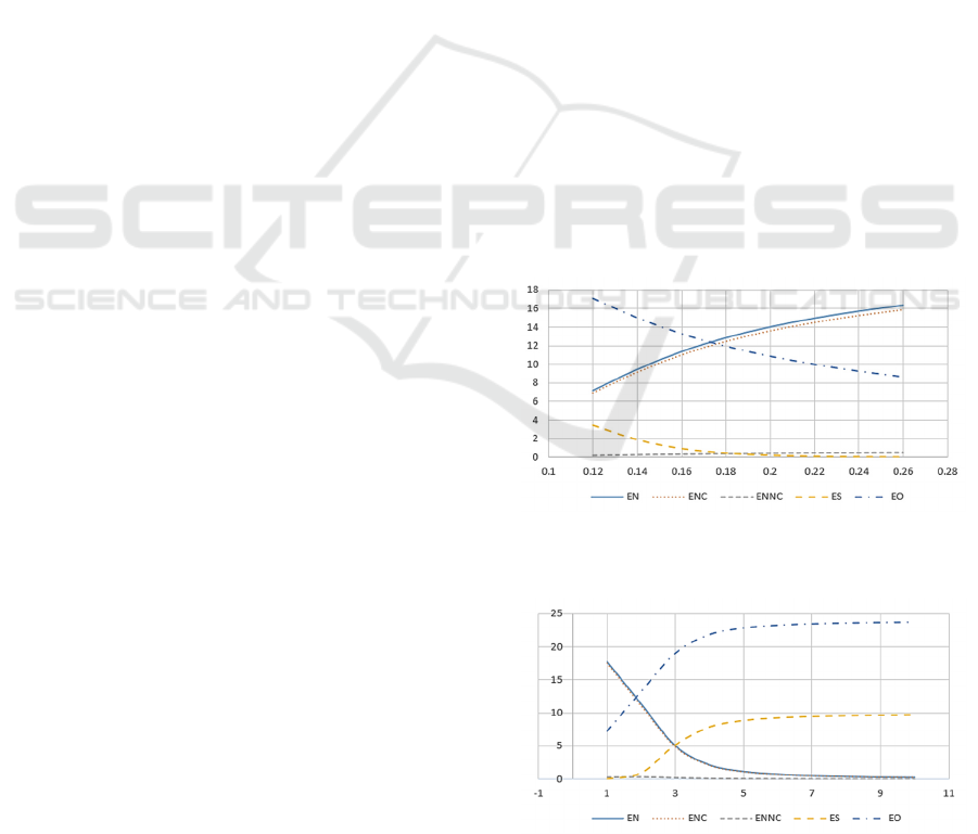
In Figure 2, we find that (i)

[]EN

[]

[]EO

, and

are significantly affected by

; (ii)

[]ES

is slightly affected by

; and (iii)

[]

and

seems too insensitive to change in

. In

Figure 3, we find that (i)

[]EN

[]

[]ES

[]EO

are significantly affected by

; and (ii)

[]

and

are slightly affected by

Figure 2: System performance measures versus various

values of

Figure 3: System performance measures versus various

values of

Cost Optimization Analysis of Retrial Machine Repair Problem with Warm Standby Components and Imperfect Coverage

305

5 COST OPTIMIZATION

ANALYSIS

Several researchers have investigated the study of

retrial queue involving cost optimization analysis.

They aimed at determining the optimal number of

servers, optimal service rate, optimal repair rate, and

so on. We construct the expected cost function per

unit time for the RMRP with warm standby

components and imperfect coverage where

and

are decision variables. Our main goal is to

determine the optimal value of

(, ,)S

μγ

, say

(, ,)S

μγ

, so as to minimize the cost function. The

cost elements are defined as follows:

C ≡

cost per unit time per failed component in the

retrial orbit when the system is in a safe failure

state (cover);

C ≡

cost per unit time per failed component in the

retrial orbit when the system is in an unsafe

failure state (not cover);

C ≡

cost per unit time of probability of

;

C ≡

cost per unit time of unavailability

1 AV−

;

C ≡

cost per unit time of providing the service rate

;

C ≡

cost per failed component in retrial orbit by

providing the retrial rate

Based on all of the cost elements listed above,

the expected cost per unit time is constructed as

follows:

12 3

(, ,) [ ] [ ]

(1 ) .

CNCNC

TC S C E N C E N C P

C AV C +C

μγ

=+ +

+−+

(25)

Thus, the cost minimization problem can be

expressed mathematically as

(, ,) (, ,).

TC S Minimize TC S

μγ

μγ μγ

5.1 Sensitivity Analysis

As the following numerical examples, we consider

the cost elements as follows:

12 3 56

$60, $12 , $2 , $48 , $9 , $3 .

CC0C40C0C0C0== = = ==

To examine the effect of system parameters on

the cost function, a sensitivity analysis in six cases is

provided for

M=15

with various values of

S = 3, 5, 7,

respectively.

Case 1:

2.0

0.08

6.0

15.0

0.9c =

varies from 0.12 to 0.26;

Case 2:

0.16=

0.08

6.0

15.0

0.9c =

varies from 1.0 to 10.0;

The numerical results of the above four cases are

shown in Figures 4-5, which depicts the sensitivity

performance of cost function

o n

, a n d

, respectively. It is important to note

that the sign of sensitivity indicates an increase or

decrease in the expected cost by changing the values

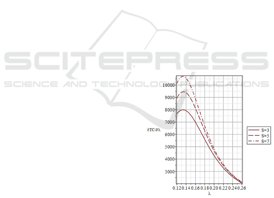
of system parameters. Figure 4 reveals that (i)

/TC

∂∂

is positive, which means that

increases as

increases for all

; (ii)

/TC

∂∂

has the highest point at around

0.13

for all

;

and for (iii), as

is fixed,

/TC

∂∂

gets larger as

increases. Figure 5 shows that (i)

/TC

∂∂

changes from negative to positive, which means that

changes from a decrease to an increase on

for all

; (ii) as

is fixed,

/TC

∂∂

gets

smaller as

increases; and when (iii) as

i s

greater than 4,

/TC

∂∂

is similar for all

Figure 4: Sensitivity analysis of

with respect to

for different

ICORES 2025 - 14th International Conference on Operations Research and Enterprise Systems

306

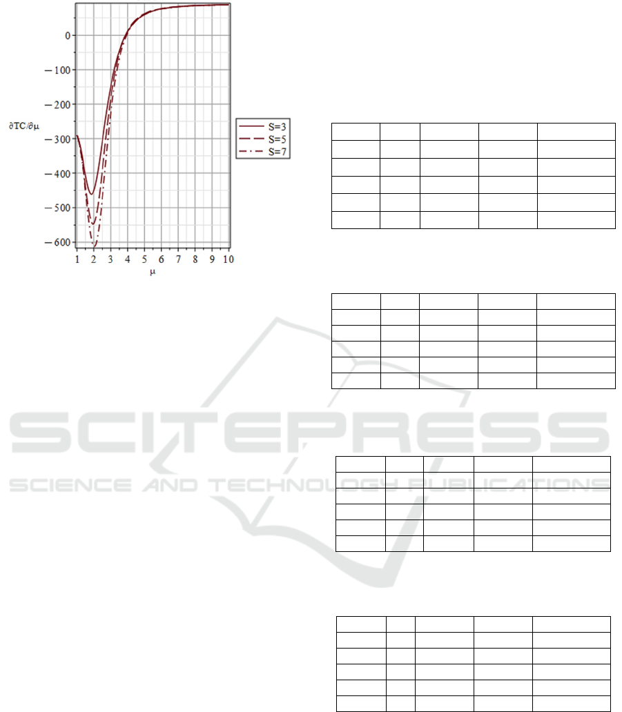
Figure 5: Sensitivity analysis of

with respect to

for different

5.2 Cost Optimization

The PSO algorithm was first proposed by Kennedy

and Eberhart (1995) and works with a population of

particles where one procedure includes exploitation

optimization searches. As the following numerical

examples, we consider the cost elements as follows:

12 3

$60, $12 , $2 ,

$48 , $9 , $3 .

CC0C40

C0C0C0

== =

===

The PSO algorithm is applied to find the approximate

optimization solution

,,(S )

μγ

and minimum cost

(, ,)TC S

μγ

. Since the PSO algorithm does not need

to compute the gradient, it is flexible for non-

differentiable cost functions. Moreover, it can be

implemented to handle optimization problems with a

mixture of discrete and continuous decision variables.

We first fix

and consider various values of

, and

. Then, after setting the different

ranges of decision variables

110S≤≤

0.1 10.0

≤≤

, a n d

0.1 20.0

≤≤

, w e

use computer software Maple for numerical

investigation. The detailed optimal solution

(, ,)S

μγ

, minimum cost

(, ,)TC S

μγ

and related

parameters are shown in Tables 1-4. We observe from

Tables 1-4 that (i) the optimal number of warm

standby components

increases as

increases;

(ii) the optimal number of warm standby components

decreases as

increases; (iii) the optimal

number of warm standby components

is the same

even though

varies from 4.0 to 8.0 and

varies

from 0.6 to 1.0; (iv)

(, ,)TC S

μγ

increases as

increases; and (v)

(, ,)TC S

μγ

decreases as

increases. Intuitively, the optimal number of

warm standby components

is significantly

affected by

and

, but seems too insensitive to

change in

and

Table 1: The optimal results for various values of

with

0.08

6.0

, and

0.9c =

(, ,)TC S

μγ

0.12 4 3.435 2.493 519.127

0.14 5 3.854 2.711 579.451

0.16 5 4.268 2.967 637.675

0.18 5 4.672 3.216 694.645

0.20 5 5.066 3.457 750.483

Table 2: The optimal results for various values of

with

0.16

6.0

, and

0.9c =

(, ,)TC S

μγ

0.04 6 4.215 2.899 622.923

0.06 5 4.247 2.957 631.115

0.08 5 4.268 2.967 637.675

0.10 5 4.288 2.976 644.031

0.12 4 4.300 3.052 648.612

Table 3: The optimal results for various values of

with

0.16

0.08

, and

0.9c =

(, ,)TC S

μγ

4.0 5 4.272 2.977 644.166

5.0 5 4.270 2.971 640.304

6.0 5 4.268 2.967 637.675

7.0 5 4.267 2.964 635.770

8.0 5 4.266 2.962 634.327

Table 4: The optimal results for various values of

with

0.16

0.08

, and

6.0

(, ,)TC S

μγ

0.6 5 4.242 3.346 689.743

0.7 5 4.250 3.223 673.331

0.8 5 4.259 3.096 656.009

0.9 5 4.268 2.967 637.675

1.0 5 4.279 2.834 618.210

6 CONCLUSIONS

This article considers the RMRP with warm standby

components and imperfect coverage. Steady-state

results are computed numerically with the matrix-

analytic technique. We have performed the sensitivity

analysis of system performance measures with

Cost Optimization Analysis of Retrial Machine Repair Problem with Warm Standby Components and Imperfect Coverage

307

respect to various system parameters. By using the

PSO algorithm, we determine the joint optimal values

of the number of warm standbys, the repair rate, and

the retrial rate simultaneously to minimize the

expected cost. The PSO algorithm can be applied to

analyze the complex optimization problems that

occur in various retrial queues (or RMRP). Under

optimal operating conditions, we illustrate our results

by discussing several cases of numerical examples.

The experimented results are helpful for managers to

make decisions. Moreover, the results obtained

provide further insight into the RMRP with warm

standby components and imperfect coverage.

REFERENCES

Artalejo, J. R. (1999a). Accessible bibliography on retrial

queues. Mathematical and Computer Modelling: An

International Journal, 30(3-4), 1-6.

Artalejo, J. R. (1999b). A classified bibliography of

research on retrial queues: progress in 1990–1999. Top,

7(2), 187-211.

El-Sherbeny, M. S., & Hussien, Z. M. (2019). Cost analysis

of series systems with different standby components

and imperfect coverage. Operations Research and

Decisions, 29(2), 21-41.

Falin, G. (1990). A survey of retrial queues. Queueing

systems, 7, 127-167.

Jain, M., & Meena, R. K. (2017). Fault tolerant system with

imperfect coverage, reboot and server vacation. Journal

of Industrial Engineering International, 13, 171-180.

Kennedy, J., & Eberhart, R. (1995, November). Particle

swarm optimization. In Proceedings of ICNN'95-

international conference on neural networks (Vol. 4, pp.

1942-1948). ieee.

Neuts, M. F. (1981). Matrix Geometric Solutions in

Stochastic Models: An Algorithmic Approach, The

John Hopkins University Press, Baltimore.

Wang, K. H., Liou, C. D., & Lin, Y. H. (2013). Comparative

analysis of the machine repair problem with imperfect

coverage and service pressure condition. Applied

Mathematical Modelling, 37(5), 2870-2880..

Wang, K. H., Su, J. H., & Yang, D. Y. (2014). Analysis and

optimization of an M/G/1 machine repair problem with

multiple imperfect coverage. Applied Mathematics and

Computation, 242, 590-600.

Wang, K. H., Wang, J., Liou, C. D., & Zhang, X. (2019).

Particle swarm optimization to the retrial machine

repair problem with working breakdowns under the N

policy. Queueing Models and Service Management,

2(1), 61-82.

Wang, K. H., Yen, T. C., & Fang, Y. C. (2012). Comparison

of availability between two systems with warm standby

units and different imperfect coverage. Quality

Technology & Quantitative Management, 9(3), 265-

282.

Wang, K. H., Yen, T. C., & Jian, J. J. (2013). Reliability and

sensitivity analysis of a repairable system with

imperfect coverage under service pressure condition.

Journal of Manufacturing systems, 32(2), 357-363.

Wu, C. H., Yen, T. C., & Wang, K. H. (2021). Availability

and comparison of four retrial systems with imperfect

coverage and general repair times. Reliability

Engineering & System Safety, 212, 107642.

Yang, D. Y., Chen, Y. H., & Wu, C. H. (2020). Modelling

and optimisation of a two-server queue with multiple

vacations and working breakdowns. International

Journal of Production Research, 58(10), 3036-3048.

Yang, T., & Templeton, J. G. C. (1987). A survey on retrial

queues. Queueing systems, 2, 201-233.

Yen, T. C., & Wang, K. H. (2020). Cost benefit analysis of

four retrial systems with warm standby units and

imperfect coverage. Reliability Engineering & System

Safety, 202, 107006..

Zhang, Y., & Wang, J. (2017). Equilibrium pricing in an

M/G/1 retrial queue with reserved idle time and setup

time. Applied Mathematical Modelling, 49, 514-530.

Zhang, X., Wang, J., & Ma, Q. (2017). Optimal design for

a retrial queueing system with state-dependent service

rate. Journal of Systems Science and Complexity, 30(4),

883-900..

ICORES 2025 - 14th International Conference on Operations Research and Enterprise Systems

308