Coordinates Transformed Signal Compression Method (CoTSiC):
A Novel Algorithm for Tele-Medicine Applications
Soham Pawar
a
and Madhav Rao
b
International Institute of Information Technology Bangalore, Bangalore, India
Keywords:
Tele-Medicine, Graph-Inspired Compression, Signal Compression, Image-Based Signal Compression.
Abstract:
Robust Telemedicine refers to the provision of reliable remote medical services, which primarily depends
on seamless transmission of either recorded signals or video information of patients in compressed form. A
wide range of physiological signals which are typically seen in the display monitor of medical instruments
including ECG, Blood Pressure, Oxygen levels, EEG signals and others are beneficial if remotely transmitted
through reliable channels. Conventionally, the compression techniques applied to the signals are complex
and compute-intensive, making it rarely viable at the remote patients’ end, where the compute infrastructure
is scarcely available. To address this challenge, the paper introduces a lightweight compression algorithm
specifically designed for these tele-healthcare applications. This work transforms the picture of the signal at
the source into a compressed array of data points. This array is sent to the remote healthcare facility and then
re-constructed into a minimalistic form of the signal. The proposed method offers a compression factor in the
range of 3.87× to 2.82× for a variety of signals including EEG, ECG, and SPO
2
signals. Additionally, an
acceptable SSIM of above 92.10%, and PSNR of above 40 dB is characterized for the reconstructed image of
different physiological signals investigated.
1 INTRODUCTION
Continuous Health Monitoring (CHM) is emerging
as a vital component of proactive healthcare (Ozkan
et al., 2020; Jiang et al., 2022; Nandi and Rao,
2022; Shaikh et al., 2023; Wu et al., 2022b). CHM
systems leverage wearable or implantable devices
for the real-time capture, analysis, or transmission
of various physiological signals (Nia et al., 2015;
Penhaker, 2022; Elhosary et al., 2019). Wearable
form factor devices (Faisal et al., 2022; Ma et al.,
2023; Chandrasekhar et al., 2020) and implantable
devices (Mart
´
ınez et al., 2023; Molloy et al., 2022),
have emerged and made significant progress in terms
of telehealth monitoring. These CHM systems are de-
signed to be unobtrusive yet effective, continuously
collecting vital physiological data, typically includ-
ing blood pressure (Nandi and Rao, 2022), oxygen
levels (Nwibor et al., 2023; Cao et al., 2012), electro-
cardiogram (ECG) (Span
`
o et al., 2016), electromyo-
gram (EMG) (Chandrasekhar et al., 2020) and elec-
troencephalogram (EEG) signals (Dabbaghian et al.,
a
https://orcid.org/0009-0008-1612-803X
b
https://orcid.org/0000-0003-2278-9148
2019; Imtiaz et al., 2019).
The advent of deep neural network (DNN)-based
methodologies has revolutionized this domain. DNNs
excel at extracting complex features from large data
sets, enabling nuanced analysis of physiological sig-
nals (Wu et al., 2022a; Doshi et al., 2021). However,
the compute-intensive nature of DNNs and frequent
data transmission needs pose challenges, especially
for less equipped centers (Luo et al., 2022). Avail-
able bandwidth often limits data transmission quality
in CHMs. In-device signal compression offers a po-
tential solution to these bandwidth challenges. How-
ever, traditional compression algorithms like least ab-
solute shrinkage (LARS) (Rudelson and Vershynin,
2006), Selection operator (LASSO) (Qaisar et al.,
2013), and Sparse Bayesian Learning (Mamaghanian
et al., 2011) are computationally intensive and un-
suitable for resource-constrained setups. This paper
introduces a novel compression method and system
specifically designed for CHM setups.
The CoTSiC algorithm efficiently extracts sig-
nal profiles from medical monitors and transmits
pixelated positional data for the monochrome ver-
sion of the image. Supplying a text stream with 2-
dimensional (2D) positional data is expected to re-
Pawar, S. and Rao, M.
Coordinates Transformed Signal Compression Method (CoTSiC): A Novel Algorithm for Tele-Medicine Applications.
DOI: 10.5220/0013173200003911
Paper published under CC license (CC BY-NC-ND 4.0)
In Proceedings of the 18th International Joint Conference on Biomedical Engineering Systems and Technologies (BIOSTEC 2025) - Volume 2: HEALTHINF, pages 603-610
ISBN: 978-989-758-731-3; ISSN: 2184-4305
Proceedings Copyright © 2025 by SCITEPRESS – Science and Technology Publications, Lda.
603

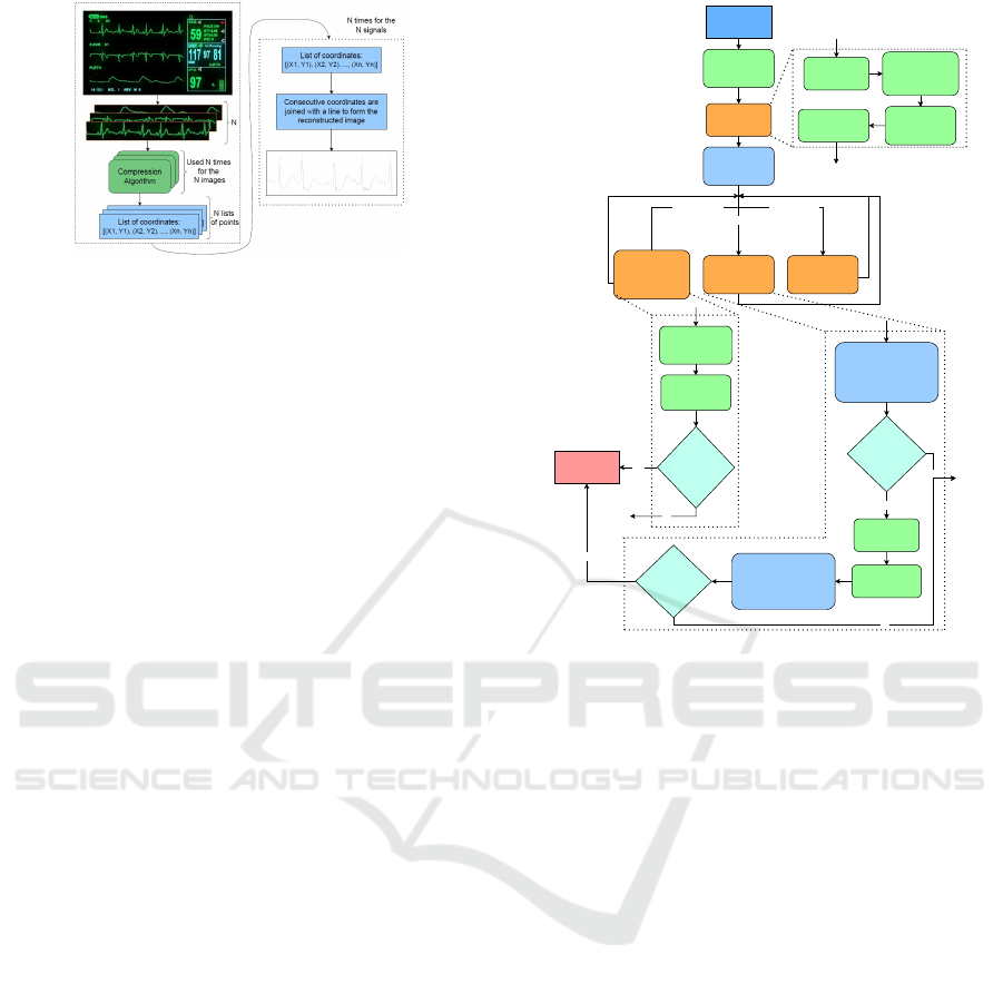
Figure 1: Schematic showing the overview of the proposed
Coordinates Transformed Signal Compression method
(left), which operates on the medical instrument display
units for CHM applications, along with the reconstructed
image formed (right) by connecting the consecutive data
points by a line.
duce both transmission and memory costs. Conven-
tional CS approaches treat compression and recon-
struction as separate processes, often leading to inef-
ficiencies (Shoaib et al., 2014). Modern web cameras
with wide coverage and depth are equipped to contin-
uously capture monitor images, transferring pixelated
data for remote signal reconstruction. The CoTSiC
scheme, depicted in Figure 1, overcomes the limita-
tion of CS methodologies where compressed signals
are not readily available for direct analysis. In con-
trast, CoTSiC transforms data into a pictorial domain,
where pixelated data is crucial for reconstruction. The
CoTSiC method offers three benefits: i) Flexibility
and compatibility with various platforms, including
workstations, smartphones, and edge computing; ii)
Independence from specific medical instruments, ap-
plicable to any diagnostic platform displaying signals;
iii) Versatility across different signals, validated for
ECG, SpO
2
, and EEG signals.
2 PROPOSED METHOD
The proposed CoTSiC scheme follows six major steps
which is illustrated in the Figure 2, and individual
steps are further discussed.
2.1 Image Preparation
The image is blurred by employing an averaging
scheme across the entire image. The kernel size of
5, configured with equal weightage to all parameters
of the kernel shows that each pixel is shared equally
across all 8 neighbours, leading to a blurred image.
The scaling factor was applied to normalize the pixel
levels according to the size chosen. This image is then
converted to a grayscale image using Otsu’s binariza-
Image Input
Image
Preparation
Process
len(coords) = 0 len(coords) > 1
Get first set of
coordinates
Localization
Re-centering the
localization
window
Finding
Junctions
Succeeding
Data Point
Get list of
unique
coordinates
Re-check if the
returned list of
coordinates is
empty
'Next Straight
Coordinates' for
each point
Re-centering
the localization
window
Finding
Junctions
Yes
List of
returned points
is empty
End of current
iteration
Remove that point from
the list which was
already covered in last
5 traversed points
Rendering
Line Width
Yes
No
Length of
new list of
points = 0
Succeeding
Data Point
len(coords) = 1
Update list of
last 5 traversed
coordinates
Remove that point from
the list which was
already covered in last
5 traversed points
No
Yes
Length of
new list of
points = 0
No
A.
B. C.
D. F.
C.
F.
E.
D.
Figure 2: Flowchart showing the proposed CoTSiC method
for extracting sequence of points from a given image.
tion scheme (Xue and Titterington, 2011). A bound-
ary of 27 pixels is then added to this image and further
converted into a two-dimensional (2D) array and re-
tained.
The stored array is operated upon by the Harris
Corner detection algorithm to get the list of all the
corner points and the set of other points associated
with each of these corner points. Post corner detec-
tion, the algorithm finds the nearest valid points from
the upper-left corner of the image. This is infused as
the starting position to trace the signal from a given
image.
2.2 Localization
Localization attempts to find the most nearest point
as mentioned above with the help of an expanding
square-shaped boundary whose upper-left corner is
fixed at that of the image. The expansion stops when
the boundary finds a pixel above the threshold value.
Figure 3 exhibits the working of a localization scheme
where the progression of an enlarging square de-
tects the features in the image. The enlarging square
boundary starts with a size of 0 and keeps increasing
with one unit (the active boundary is shown in blue,
and the previous boundary is in yellow).
HEALTHINF 2025 - 18th International Conference on Health Informatics
604

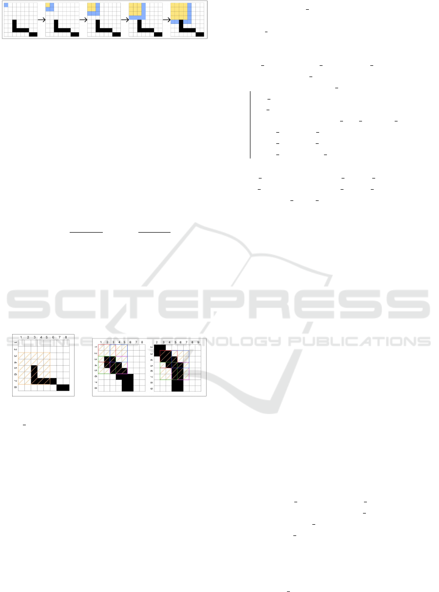
Figure 3: Progression of enlarging square boundary for
finding nearest non-zero pixel for a given image.
2.3 Re-Centering the Localizing
Window
This step is applied to find the best square window
that maximizes the captured pixelated data, given the
extracted pixel positions and size of the enlarging
square. The centre of intensity (COI) is computed
and the centre point is repositioned based on the com-
puted COI. The coordinates of COI (Center of Inten-
sity) is expressed as the weighted average of intensity
along X and Y coordinates, also expressed below in
the Equation 1.
X
COI
=
∑
n
i=1
I
i
X
i
∑
n
i=1
I
i
,Y
COI
=
∑
n
i=1
I
i
Y
i
∑
n
i=1
I
i
(1)
This COI is computed and stored for uniquely iden-
tifying the location of different Harris corners later
in the process when required. Another use of reposi-
tioning is to find the best point such that the deduced
contours are uniformly distributed and are as accurate
as possible. The resulting 3D plot is centered around
the adjusted coordinates.
Figure 4: Tempo-
rary square in Gra-
pher 3D module, en-
larged to extract the
collection of points
in the square.
Figure 5: Representation of four
quadrants for finding the direc-
tion and best-fit line with respect
to the succeeding pixel.
2.4 Succeeding Data Point
This step identifies the following pixelated coordinate
position, given the current center point and its direc-
tion with respect to the preceding point. This step
assumes a square of fixed length defined by its center
location as first input. It iterates through all the coor-
dinates and checks whether any of the pixels are a part
of Harris corner. If any Harris corners are detected,
the directions and coordinates for multiple possible
paths are stored. If not, then the current square un-
der processing contains only a single path without
any sharp edge, thereby a best-fit line is drawn to the
Input: window size: Size of the window
center: Center point of current window
IMG F: 2D matrix of intensities from image
Output: point: Center point of re-centered
window
sum ints ← 0, sum X ← 0, sum Y ← 0;
mid ← (window size − 1)/2;
for x,y ← 0 to window size − 1 do
X temp ← center
x
− mid + x;
Y temp ← center
y
− mid + y;
value ← 255 − IMG F[Y temp][X temp];
sum X ← sum X + (x − mid) · value;
sum Y ← sum Y + (y − mid) · value;
sum
ints ← sum ints + value;
end
CX T ← center
x
+ ⌊sum X/sum ints⌋;
CY T ← center
y
+ ⌊sum Y /sum ints⌋;
return [CX T,CY T ];
Algorithm 1: Re-center Window (Block C).
next coordinate. For instance, in the Figure 5 shown,
if the current location of (5,5) and the direction of
’SE’ (South-East) is given, then a line extends from
the current position to the succeeding coordinate (6,6)
with the direction ’S’ (South). Figure 5 illustrates the
square size of 5×5 pixels. Here, the blue-coloured
square inside the bigger shaded square is considered
quadrant 1 (Q1), red is Q2, green is Q3 and pink is
Q4. Hence, all coordinates and its directions are com-
puted based on the quadrants considered. The mov-
ing square then centres to this new point, but the co-
ordinates considered for the new position remains to
be Q1, Q3 and Q4. This is because, for the previ-
ous point, the direction computed was ’SE’ and hence
in the new position of square, the direction of ’NW’
points to Q2 and the same is not considered to find the
new best-fit line. Once the slope of the best-fit line is
computed, the farthest point among all from the quad-
rants considered with the same slope is picked for ren-
dering the signal. This new point is then employed
to compute the coordinates of a next point in the se-
quence such that it lies exactly at the center of the line
width while rendering the signal.
Input: IMG F, CX , CY , KER SIZE,
LIMIT , PREV, PREV COORDS,
IGNORE HARRIS
Output: f p f QS
opp ← {SW : [Q2, Q3,Q4],W :
[Q2,Q3],NW : [Q1,Q2,Q3], N :
[Q1,Q2],NE : [Q1,Q2, Q4],E :
[Q1,Q4],SE : [Q1, Q3,Q4],S : [Q3,Q4]};
s ← (KER SIZE − 1)/2;
x,y,vals,Q1, Q2,Q3, Q4 ←
/
0;
Coordinates Transformed Signal Compression Method (CoTSiC): A Novel Algorithm for Tele-Medicine Applications
605

Q(x,y) ←













Q1,2 if x == CX ∧ y < CY
Q3,4 if x == CX ∧ y > CY
Q2,3 if y == CY ∧ x < CX
Q1,4 if y == CY ∧ x > CX
Q1,2,3,4 if [x,y] == [CX,CY]
;
for Y ← (CY − s) to (CY + s) do
for X ← (CX −s) to (C X +s) do
value ← IMG F[Y ][X];
if value < LIMIT then
intensity ← (255 − value)/255;
x ← x ∪ {X}, y ← y ∪ {Y };
vals ← vals ∪ {intensity};
v coords ← v coords ∪ [X,Y ];
if X == CX or Y == CY then
add [X,Y,intensity] to
Q(X,Y );
else
add [X,Y,intensity] to the
corresponding quadrant
array;
end
end
end
end
if PREV is not empty then
f inal QS ←
S
elements in quadrant
arrays present in opp[PREV ];
end
else
f inal QS ← Q1
S
Q2
S
Q3
S
Q4;
end
wmean x f QS, wmean y f QS ← 0;
f inal QS, pp, pp f QS, f p f QS ←
/
0;
bb f ← slope of best fit line for v coords;
bb f ← max(bb f ,10
−7
)
angle f QS ← arctan(bb f );
dir gen f QS ← Algorithm 5(angle f QS);
for (x,y,val) ∈ f inal QS do
p1, p2 ← end-points of best fit line within
the current window;
if (p1
x
== x ∨ p2
x
== x ) ∨ (p1
y
==
y ∨ p2
y
== y) then
pp f QS ← pp f QS ∪ {[x,y]};
end
end
Algorithm 2: Next Data Point (Block D).
2.5 Rendering Line Width
As shown in the Figure 6, the triangle formed from the
farthest point in the vertical and horizontal direction
each also highlighted by green line, aids in finding the
length of the purple line (line thickness).
Figure 6: Illus-
tration, depicting
the estimation of
line width.
Figure 7: Contour lines for
case#1 (left): Around a Harris
Corner point and case#2 (right): when
no coordinates for the next point are
found.
for point ∈ pp f QS do
angle curr ← arctan

point
y
−CY
point
x
−CX

;
direction ← Algorithm 5(angle curr );
if direction ̸= dir gen f QS then
remove point from pp f QS;
end
end
if current window has a Harris Point then
f p f QS ← Algorithm 8(point)∀ points in
the window;
end
else
forall point ∈ pp f QS do
f p f QS ←
f p f QS ∪ Algorithm 6(point);
end
end
return f p f QS;
Algorithm 3: Next Data Point (Block D) - Continuation.
Input: angle
Output: dir
dir ← ’E’;
if angle ∈ [0.125, 0.375] ∪ [−0.875,−0.625] then
dir ← ’SE’;
end
else if angle ∈ [0.375, 0.625] ∪ [−0.625,−0.375]
then
dir ← ’S’;
end
else if angle ∈ [0.625, 0.875] ∪ [−0.375,−0.125]
then
dir ← ’SW’;
end
return dir;
Algorithm 4: Direction Pointing Function.
2.6 Finding Junctions
The Succeeding Data step presents several points
defining different paths for junction points, and their
corresponding directions in case the region under
study comprises of Harris corners. The contour lines
for that region is found initially. A Pre-processing
step is applied to ensure that the thickness of the line
HEALTHINF 2025 - 18th International Conference on Health Informatics
606

Input: point, beta bar, img f , limit, length
Output: f p
possible ←
/
0;
xc,yc ← point;
l xc,u xc ← xc;
l yc,u yc ← yc;
while img f [yc][l xc − 1] <
limit ∧ |x c − l xc + 2| ≤ length do
l xc ← l xc − 1;
end
while img f [yc][u xc +1] <
limit ∧ |u xc − xc + 2| ≤ length do
u xc ← u xc + 1;
end
do the same decrement and increment for l yc
and u yc in the y-direction;
range o f points ←
/
0;
for x ← l xc to u xc do
for y ← l yc to u yc do
add [x,y] to range o f points;
end
end
b ← |u yc −l yc|, a ← |u xc − l xc|;
compute the line perpendicular (pink) to the
hypotenuse (green) using the construction in 6
and a,b;
p1, p2 ← end-points of the line with intensity
< limit;
f p ← mid-point of p1 and p2;
return f p;
Algorithm 5: Find Maximum Perpendicular Point (Block
E).
Input: curr points: List of points for which the
ends of the path are to be calculated
Output: points: Coordinates of re-centered
window
contours ← get contour lines for curr points;
end points, points ←
/
0;
for lines ∈ contours do
add end points of lines to end points;
end
hull ← convex hull generated from points in
end points;
group ← pairs of points from hull, each from
consecutive contour lines, ensuring closest
possible points;
for g ∈ group do
add the mid-point of points in g to points;
end
return points;
Algorithm 6: Finding Junction Ends (Block F).
lies completely inside the assumed square and there is
a difference in the intensities of the adjacent pixels for
the contour lines. The coordinates of the end-points
for each contour line in the outermost set is noted and
re-arranged such that when drawn in the sequence,
these points form a convex polygon. The coordinates
are re-arranged by first finding the mean of the cor-
responding X and Y values in the coordinate system,
also referred to as centroid. Then the polar angles of
each of the points with respect to its centroid is com-
pared and sorted. Figure 7 depicts contour lines for
two cases when the Harris corner is detected and oth-
erwise. In the left image, this method was used be-
cause a junction was found through the Harris corner
detection process. The Harris coordinates are repre-
sented by yellow color. The colored dots at the end
are the points computed for generating contour lines.
In each of the images depicted in the Figure 8, the
circles indicate that among all the contour lines, the
one which lies on the outermost boundary is selected.
These are chosen to form a convex polygon, and are
Figure 8: Pairing of end-points of consecutive contour lines
in the outermost set of contours.
further paired to form corresponding paths. For ex-
ample, in Figure 8, the pairs (upper-red, upper-blue),
(lower-blue, right-green) and (left-green, lower-red)
correspond to the end-points of the three contour
lines. For each pair, the mean point is calculated
and shown in Figure 7. Once the list of coordinates
are available, the points that have crossed the bound-
ary of the paths are excluded. The boundary points
are just the lines connecting the end-points forming
the pair. Care is taken to prevent from traversing the
same path for more than once. The crossed bound-
ary lines are found out by scanning the list of the last
5 traversed points and comparing their relative posi-
tions with each of the boundary lines. The boundary
line is identified by zero crossing algorithm where the
product of successive traversed coordinates emerges
to negative, and the corresponding coordinates of the
point and the direction is removed from the computed
list.
3 EVALUATION
The advantages of this proposed CoTSiC method is
the possibility of reconstructing images to any possi-
ble size. SSIM metric requires both original and re-
constructed image of same size. Hence for different
sizes, both images are first resized to a common di-
mension. This image is scaled down to the desired
dimension and then supplied to the proposed method
for extracting the reconstructed image. It was evident
Coordinates Transformed Signal Compression Method (CoTSiC): A Novel Algorithm for Tele-Medicine Applications
607

from experimental evaluation that as the common di-
mension of the signal image increases, the SSIM im-
proves. The SSIM score for the original dimension
is reported to be 92.14%, with a PSNR of 44.72 dB,
which is acceptable (Setiadi, 2021).
(a) Original image (831x710) (b) Reconstructed image (831x710)
Figure 9: Input image vs reconstructed images.
Figure 10 (a) shows the input ECG signal, and
the image of the reconstructed signal. The recon-
structed image and the original image have the same
dimensions exhibiting SSIM of 97.08%, and PSNR of
48.75 dB. Figure 11 shows the theta and delta compo-
nents of the original EEG signal, and the image of
the reconstructed signal respectively. Figure 10 (b)
shows the original SpO2 signal with motion artifact,
and its corresponding reconstructed signal. The re-
constructed and the original image have the same
dimensions exhibiting SSIM of 95.23%, and PSNR
of 43.12 dB. Similarly, SPO
2
signal with no mo-
tion artifact generates SSIM of 97.3%, and PSNR of
46.53 dB. Table 1 compares the SSIM and PSNR val-
ues between images post JPEG compression and im-
ages formed after reconstruction from the data points
generated by the proposed method for input images
covering different physiological signals. Table 2 sum-
marizes SSIM for all the investigated signals, and its
compression benefits. The compression factor is esti-
mated as the ratio of file size of original image and the
corresponding reconstructed image. The compression
factor in the range of 3.87× to 2.82× is characterized
for the proposed CoTSiC method for four different
signals with SSIM and PSNR of more than 92.10%,
and 40 dB PSNR respectively.
Figure 10: (a) ECG (left) and (b) SpO
2
(right) signals: input
(top) reconstructed signals (bottom).
Figure 11: (a) Theta (left) and (b) Delta (right) components
of an EEG Signal: input (top) reconstructed signal (bottom).
4 COMPLEXITY ANALYSIS
The complexity of image preparation process is ex-
pressed as:
O(M × N × k
2
)
| {z }
Term 1
+O(N
2
)
| {z }
Term 2
+O(W
2
)
| {z }
Term 3
+O(W
2
)
| {z }
Term 4
+O(W
2
)
| {z }
Term 5
In this Equation , M and N are the input image dimen-
sions and k is the blur kernel size in Term 1 and Term
2. k is a constant and thus can be ignored from the
term. In Term 3, Term 4 and Term 5, W represents
the window size which is used for estimating the data
points. In Term 5, W
2
is required since all the points
in the window are required for calculating the junc-
tion end-points. Following this, the equation can be
written as:
O(M × N)
| {z }
Term 1
+O(N
2
)
| {z }
Term 2
+ 3 O(W
2
)
| {z }
Term 3
Thus, the complexity of the image pre-processing
portion of the whole algorithm is O(M × N). For
the recursive part of the algorithm, there are three
branches possible. For each iteration, the cost func-
tion is stated in the Equation 2.
T (P
i
) =
{p
j
}
∑
k
(O(W
2
[P
i
,P
k
]
) + T (P
k
)) (2)
Here, a path is defined as the signal waveform along
which the shifting window of dimension W ×W pix-
els, traverses. This window estimates the next coordi-
nates based on only that portion of the path which lies
inside the window, thus leading to the greedy nature
of the algorithm. O(W
2
[P
i
,P
k
]
) represents the time com-
plexity of these operations where P
i
and P
k
are the
start and end points of the portion of path currently
inside the window. T (P
i
)) represents the time com-
plexity corresponding for the path with P
i
as the start
point. For case len(coords = 1), {p
j
} = i + 1. The
equation simplifies to T ([P
i
,P
n
]) = 2O(W
2
[P
i
,P
i+1
]
) +
T (P
i+1
) For case len(coords = 0), the equation simpli-
fies to T([P
i
,P
n
]) ≈ 2O(W
2
[P
i
,P
i+1
]
) For case len(coords
> 1), {p
j
} = i + 1, the time complexity is further
simplifies to T (P
i
) =
∑
{p
j
}
k
(O(W
2
[P
i
,P
k
]
) + T (P
k
)) Here
{p
j
} represents the set of start points for the new
branching paths. All these cases are referred to Fig-
ure 12.
Complexity analysis of the overall recursion is
done by considering the worst-case for the input im-
age. This is where the physiological signal image
contains as many peaks as possible and covers the
most portion of the image frame. The closer the arms
of the peaks (Figure 13) are, the more number of
peaks are accommodated in the image. Experimen-
tally, it was found that the minimum distance between
HEALTHINF 2025 - 18th International Conference on Health Informatics
608

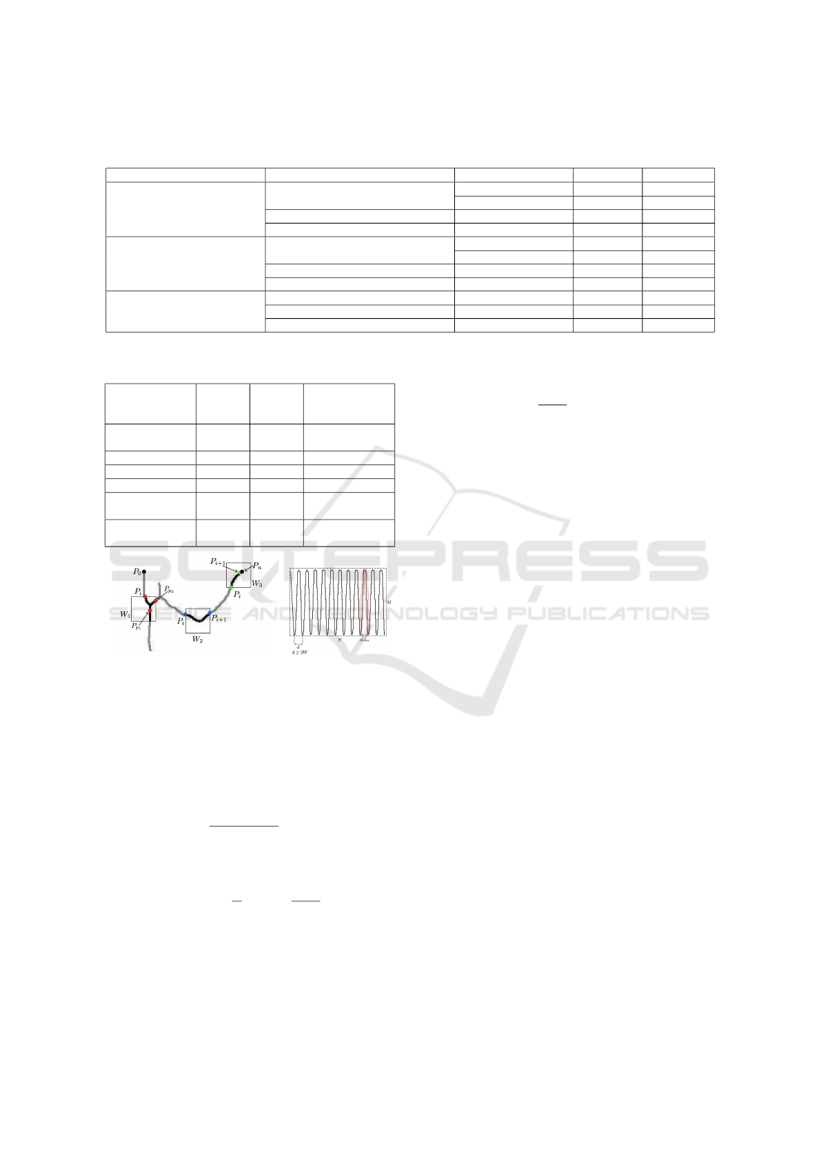
Table 1: SSIM and PSNR metrics comparison for different images post JPEG compression and those reconstructed from the
proposed CoTSiC method.
Signal Generator Reconstructed Image Resized Dimensions SSIM (%) PSNR (db)
ECG (173 KB), 2100 × 2826
Proposed (56 KB), 2826 × 2826
2100 × 2826 97.10 48.41
2826 × 2826 97.26 48.46
JPEG Best (234KB), 2100 × 2826 2100 × 2826 99.99 71.38
JPEG Least (100KB), 2100 × 2826 2100 × 2826 99.55 44.91
EEG (224KB), 1341 × 4626
Proposed (69KB), 1341 × 4626
1341 × 4626 95.41 57.31
2313 × 2313 93.95 50.80
JPEG Best (325KB), 1341 × 4626 1341 × 4626 98.53 44.25
JPEG Least (121KB), 1341 × 4626 1341 × 4626 98.53 44.25
SpO2 (82KB) 294 × 1707
Proposed (11KB), 294 × 1707 2904 × 1707 81 36.90
JPEG Best (82KB), 294 × 1707 294 × 1707 99.94 60.35
JPEG Least (18KB), 294 × 1707 294 × 1707 98.02 39.90
Table 2: SSIM estimated for the CoTSiC method generated
re-constructed physiological signals.
Signal SSIM
Score
PSNR Compression
Ratio (same
dimensions)
Sample signal
(Fig. 9)
92.14% 44.72dB 2.82
ECG 97.08% 48.75dB 3.39
Theta EEG 95.02% 58.8dB 3.5
Delta EEG 92.86% 40.71dB 3.87
SpO2 with Mo-
tion Artifact
95.23% 43.12dB 3.28
SpO2 with no
Motion Artifact
97.3% 46.53dB 3.45
Figure 12: Schematic of phys-
iological signal with windows
W
1
, W
2
, and W
3
for the three
T ([P
i
,P
n
]) conditions stated
above. P
0
and P
n
are the start
and end points.
Figure 13: Worst
case image input
(M × N), where the
peak height is the
image height M.
the base of the arms of a peak should be at least 2×W .
This was tested with different line widths of the sig-
nal. Assuming an approximate straight arm and using
simple trigonometry, for the worst case, the number
of peaks and arm length is expressed as n
peaks
= N/d,
and l
arm
= M ×
q
1 +




:
0
(W /M)
2
respectively. Since
W ≪ M, the path length of the whole waveform is
written as:
l
path
= 2n
peaks
l
arm
≈
N
d
(2M) =
2MN
d
= kMN (3)
Grouping all constants, the number of new posi-
tions taken by the window while traversing the path
is:
n
opers
= l
path
/W = (kMN)/W
Considering time complexity of window operations,
the total time complexity is:
n
opers
· O(W
2
) =
kMN
W
· O(W
2
) = O(MN W ) (4)
Considering W as a constant, the complexity becomes
O(M × N) Hence the overall time complexity of the
proposed method is deduced to 2O(M × N) = O(M ×
N), better than LASSO and Sparse Bayesian Learning
algorithms Where M and N are the dimensions of the
input image.
5 CONCLUSIONS
This study presents a novel signal compression
scheme leveraging image processing to convert im-
age(s) of signals from medical instrument displays
into arrays of data points, requiring minimal ad-
ditional setup for tele-healthcare. By avoiding
machine learning algorithms, the method supports
low-resource edge computing, making it viable for
resource-constrained environments. Future work in-
cludes optimizing the algorithm by processing images
in smaller blocks to reduce computational overhead
and developing a mobile application compatible with
a wide range of devices, enhancing accessibility and
practicality for telemedicine.
REFERENCES
Cao, Z., Zhu, R., and Que, R.-Y. (2012). A wireless portable
system with microsensors for monitoring respiratory
diseases. IEEE Transactions on Biomedical Engineer-
ing, 59(11):3110–3116.
Chandrasekhar, V., Vazhayil, V., and Rao, M. (2020). De-
sign of a real time portable low-cost multi-channel
surface electromyography system to aid neuromus-
cular disorder and post stroke rehabilitation patients.
In 2020 42nd Annual International Conference of the
Coordinates Transformed Signal Compression Method (CoTSiC): A Novel Algorithm for Tele-Medicine Applications
609

IEEE Engineering in Medicine & Biology Society
(EMBC), pages 4138–4142.
Dabbaghian, A., Yousefi, T., Fatmi, S. Z., Shafia, P., and
Kassiri, H. (2019). A 9.2-g fully-flexible wireless
ambulatory eeg monitoring and diagnostics headband
with analog motion artifact detection and compensa-
tion. IEEE Transactions on Biomedical Circuits and
Systems, 13(6):1141–1151.
Doshi, R., Sankar, A. R., Nagaraj, K., Vazhayil, V., Nagaraj,
C., and Rao, M. (2021). Eeg driven autonomous in-
jection system for an epileptic neuroimaging applica-
tion. In 2021 43rd Annual International Conference of
the IEEE Engineering in Medicine & Biology Society
(EMBC), pages 1480–1486.
Elhosary, H., Zakhari, M. H., Elgammal, M. A., Abd
El Ghany, M. A., Salama, K. N., and Mostafa, H.
(2019). Low-power hardware implementation of a
support vector machine training and classification
for neural seizure detection. IEEE Transactions on
Biomedical Circuits and Systems, 13(6):1324–1337.
Faisal, A. I., Mondal, T., Cowan, D., and Deen, M. J.
(2022). Characterization of knee and gait features
from a wearable tele-health monitoring system. IEEE
Sensors Journal, 22(6):4741–4753.
Imtiaz, S. A., Iranmanesh, S., and Rodriguez-Villegas, E.
(2019). A low power system with eeg data reduction
for long-term epileptic seizures monitoring. IEEE Ac-
cess, 7:71195–71208.
Jiang, W., Majumder, S., Kumar, S., Subramaniam, S., Li,
X., Khedri, R., Mondal, T., Abolghasemian, M., Sa-
tia, I., and Deen, M. J. (2022). A wearable tele-health
system towards monitoring covid-19 and chronic dis-
eases. IEEE Reviews in Biomedical Engineering,
15:61–84.
Luo, X., Liu, D., Huai, S., Kong, H., Chen, H., and Liu, W.
(2022). Designing efficient dnns via hardware-aware
neural architecture search and beyond. IEEE Trans-
actions on Computer-Aided Design of Integrated Cir-
cuits and Systems, 41(6):1799–1812.
Ma, C., Wang, Z., Zhao, L., Long, X., Vullings, R., Aarts,
R. M., Li, J., and Liu, C. (2023). Deep learning-based
signal quality assessment in wearable ecg monitoring.
In 2023 Computing in Cardiology (CinC), volume 50,
pages 1–4.
Mamaghanian, H., Khaled, N., Atienza, D., and Van-
dergheynst, P. (2011). Compressed sensing for real-
time energy-efficient ecg compression on wireless
body sensor nodes. IEEE Transactions on Biomedi-
cal Engineering, 58(9):2456–2466.
Mart
´
ınez, S., Veirano, F., Constandinou, T. G., and Silveira,
F. (2023). Trends in volumetric-energy efficiency of
implantable neurostimulators: A review from a cir-
cuits and systems perspective. IEEE Transactions on
Biomedical Circuits and Systems, 17(1):2–20.
Molloy, A., Beaumont, K., Alyami, A., Kirimi, M., Hoare,
D., Mirzai, N., Heidari, H., Mitra, S., Neale, S. L.,
and Mercer, J. R. (2022). Challenges to the develop-
ment of the next generation of self-reporting cardio-
vascular implantable medical devices. IEEE Reviews
in Biomedical Engineering, 15:260–272.
Nandi, P. and Rao, M. (2022). A novel cnn-lstm model
based non-invasive cuff-less blood pressure estimation
system. In 2022 44th Annual International Confer-
ence of the IEEE Engineering in Medicine & Biology
Society (EMBC), pages 832–836.
Nia, A. M., Mozaffari-Kermani, M., Sur-Kolay, S., Raghu-
nathan, A., and Jha, N. K. (2015). Energy-efficient
long-term continuous personal health monitoring.
IEEE Transactions on Multi-Scale Computing Sys-
tems, 1(2):85–98.
Nwibor, C., Haxha, S., Ali, M. M., Sakel, M., Haxha, A. R.,
Saunders, K., and Nabakooza, S. (2023). Remote
health monitoring system for the estimation of blood
pressure, heart rate, and blood oxygen saturation level.
IEEE Sensors Journal, 23(5):5401–5411.
Ozkan, H., Ozhan, O., Karadana, Y., Gulcu, M., Macit, S.,
and Husain, F. (2020). A portable wearable tele-ecg
monitoring system. IEEE Transactions on Instrumen-
tation and Measurement, 69(1):173–182.
Penhaker, M. (2022). Biomedical engineering in the 21st
century and in the future. In 2022 IEEE 20th Jubilee
World Symposium on Applied Machine Intelligence
and Informatics (SAMI), pages 000011–000012.
Qaisar, S., Bilal, R. M., Iqbal, W., Naureen, M., and Lee,
S. (2013). Compressive sensing: From theory to ap-
plications, a survey. Journal of Communications and
Networks, 15(5):443–456.
Rudelson, M. and Vershynin, R. (2006). Sparse reconstruc-
tion by convex relaxation: Fourier and gaussian mea-
surements. In 2006 40th Annual Conference on Infor-
mation Sciences and Systems, pages 207–212.
Setiadi, D. R. I. M. (2021). Psnr vs ssim: imperceptibility
quality assessment for image steganography. Multi-
media Tools and Applications, 80:8423–8444.
Shaikh, M. R., Rao, M., and Subramaniam, G. (2023). A
novel thermal imaging based transfer-learning model
to estimate blood pressure. In 2023 IEEE 20th Inter-
national Symposium on Biomedical Imaging (ISBI),
pages 1–5.
Shoaib, M., Lee, K. H., Jha, N. K., and Verma, N. (2014).
A 0.6–107 µw energy-scalable processor for directly
analyzing compressively-sensed eeg. IEEE Trans-
actions on Circuits and Systems I: Regular Papers,
61(4):1105–1118.
Span
`
o, E., Di Pascoli, S., and Iannaccone, G. (2016). Low-
power wearable ecg monitoring system for multiple-
patient remote monitoring. IEEE Sensors Journal,
16(13):5452–5462.
Wu, D., Li, S., Yang, J., and Sawan, M. (2022a). neuro2vec:
Masked fourier spectrum prediction for neurophysio-
logical representation learning.
Wu, D., Yang, J., and Sawan, M. (2022b). Bridging the
gap between patient-specific and patient-independent
seizure prediction via knowledge distillation. Journal
of Neural Engineering, 19(3):036035.
Xue, J.-H. and Titterington, D. M. (2011). t -tests, f -
tests and otsu’s methods for image thresholding. IEEE
Transactions on Image Processing, 20(8):2392–2396.
HEALTHINF 2025 - 18th International Conference on Health Informatics
610