Optimal Covering and Trajectory Planning for Air-Ground Integrated
Networks in Post-Disaster Scenarios
Khouloud Kessentini
1,2 a
, Raouia Taktak
1,2 b
and Lamia Chaari
1,2 c
1
Digital Researh Center of Sfax (CRNS), Laboratory of Signals, systeMs, aRtificial Intelligence and neTworkS (SM@RTS),
Tunisia
2
Higher Institute of Computer Science and Multimedia of Sfax, University of Sfax, Tunisia
Keywords:
Air-Ground Integrated Networks (AGIN), Unmanned Aerial Vehicles (UAVs), Unsplittable Capacitated
Facility Location Problem (UCFLP), Capacitated Vehicle Routing Problem (CVRP), Mixed-Integer Linear
Programming (MILP), Variable Neighborhood Search (VNS).
Abstract:
In this paper, we examine a post-disaster scenario in which Access Points (APs) in an affected area are deac-
tivated, resulting in the disconnection of End Devices (EDs). This disruption weakens situational awareness
and impacts the overall effectiveness of rescue operations. Thus, quick network recovery becomes essential
for emergency efforts. Toward this end, Air-Ground Integrated Networks (AGIN) present new opportunities,
which this study explores by using cruising Unmanned Aerial Vehicles (UAVs) to reconnect deactivated APs
effectively. In this study, we solve this problem through a two-step process. First, we identify the best discon-
nected APs for reactivation. This subproblem is formulated as an Unsplittable Capacitated Facility Location
Problem (UCFLP). Second, we plan the UAVs paths to reactivate these selected APs. This subproblem is for-
mulated as a Capacitated Vehicle Routing Problem (CVRP). We present an Integer Linear Programming (ILP)
formulation for the UCFLP and a Mixed-Integer Linear Programming (MILP) formulation for the CVRP, then
we propose a Variable Neighborhood Search (VNS) algorithm to solve the CVRP in a reasonable amount of
time. Computational results show the efficiency of the proposed method.
1 INTRODUCTION
In the few past years, the use of Unmanned Aerial Ve-
hicles (UAVs) have witnessed a significant growth in
numerous fields including transportation, traffic con-
trol, smart agriculture, etc. One of the areas where
UAVs have emerged as a promising opportunity is
disaster recovery and rescue operations. This emer-
gence stems from the UAVs capacity to accomplish
challenging and dangerous tasks for humans such
as survivals search, firefighting, physical damage in-
spection, etc. Nevertheless, several challenges have
arisen alongside the opportunities of deploying UAVs
in these contexts. Indeed, the UAVs trajectory plan-
ning presents a significant challenge due to the com-
plexity of the task. The problem becomes substan-
tially more difficult when the disaster affects a broad
area, requiring hence the deployment of numerous
UAVs to serve a large population. Additional factors,
a
https://orcid.org/0009-0005-6474-7693
b
https://orcid.org/0000-0003-2377-5709
c
https://orcid.org/0000-0003-0401-5050
such as UAVs battery constraints, population mobil-
ity, weather conditions and limited budget constraints
add extra layers of complexity to the path planning
and deployment of UAVs.
1.1 Related Work
Several studies have explored UAVs deployment in
post-disaster scenarios, employing both exact and ap-
proximate methods to deal with the resulting opti-
mization problems. In (Calamoneri et al., 2024) for
instance, the authors examine a post-disaster emer-
gency scenario in which a fleet of UAVs assists res-
cue teams in identifying people in need of assis-
tance in the affected area. The problem is formu-
lated as a multi-depot multi-trip vehicle routing prob-
lem with total completion time minimization. The
authors present a Mixed-Integer Linear Programming
(MILP) formulation and a metaheuristic framework to
solve large instances of the problem. In (Coco et al.,
2024), the authors study the probabilistic drone rout-
ing problem and employ drones to identify victims
Kessentini, K., Taktak, R. and Chaari, L.
Optimal Covering and Trajectory Planning for Air-Ground Integrated Networks in Post-Disaster Scenarios.
DOI: 10.5220/0013173400003893
Paper published under CC license (CC BY-NC-ND 4.0)
In Proceedings of the 14th International Conference on Operations Research and Enterprise Systems (ICORES 2025), pages 309-319
ISBN: 978-989-758-732-0; ISSN: 2184-4372
Proceedings Copyright © 2025 by SCITEPRESS – Science and Technology Publications, Lda.
309

in inaccessible or hazardous areas following major
disasters. The objective function maximizes the ex-
pected number of identified individuals. Moreover,
interesting considerations are also examined in this
study, such as anti-collision constraints and allow-
ing multiple visits at an observation point. To solve
the problem, the authors propose a greedy construc-
tive heuristic as well as two Adaptive Large Neigh-
borhood Search (ALNS)-based methods. In (Chowd-
hury et al., 2021), the authors investigate the het-
erogeneous fixed fleet drone routing problem to de-
velop a safe, reliable, and cost-efficient inspection
plan for disaster-affected areas using battery-driven
drones. The study introduces a MILP to minimize
post-disaster inspection costs by incorporating drone-
related factors such as ascending and descending
costs, battery recharging requirements, and service
costs such as costs of capturing images at affected
locations. To solve large-scale instances, two algo-
rithms were proposed: ALNS and Modified Back-
tracking Adaptive Threshold Accepting (MBATA).
Computational results demonstrate that the MBATA
consistently generates high-quality solutions within a
reasonable amount of time. In (Adsanver et al., 2024),
the authors present a multistage framework designed
for post-disaster scenarios where drones are deployed
to assess physical damage to infrastructure. The dis-
aster region is divided into grids, each defined by
specific attributes, such as geographical and geolog-
ical conditions. The framework optimizes the use of
a limited number of drones, incorporating two itera-
tive phases to ensure that all grids are surveyed: (i)
Phase I focuses on solving a drone routing problem
by determining which grids should be scanned within
a limited time based on grid priorities and collected
data. (ii) In Phase II, the damage status of the un-
scanned grids is predicted based on the data collected
during Phase I. For a detailed examination on the role
of drones in disaster response, the reader can refer to
(Yucesoy et al., 2024).
1.2 Problem Statement
This study examines a post-disaster scenario in which
severe damage to wireless network infrastructure
leaves the population in the disaster area isolated
and unable to communicate with the outside world.
As illustrated in Figure 1, we consider a wireless
communication system in which some Access Points
(APs) are impacted by a disaster. These affected APs
are grouped into two categories: (1) severely dam-
aged or destroyed APs that cannot be reactivated and
are, therefore, excluded from the recovery process,
(2) partially damaged or operational but disconnected
Stable Area
Disaster Area
Û
Functional AP
Connected ED




Û
Serverly damaged AP

Disconnected EDs

ÛÛ

Disconnected AP


Figure 1: Problem structure and context representation.
APs that require reactivation by UAVs. In both cate-
gories, the End Devices (EDs) covered by these APs
are disconnected from the wireless network. We aim
to restore connectivity for the entire population of
EDs in the disaster area by reactivating the APs that
can best fulfill the overall bandwidth demands of the
EDs.
The problem is divided into two subproblems. In
the first subproblem, the optimal set of disconnected
APs should be identified. Note that an “optimal” set
of APs is defined by a total cost we aim to minimize,
which is given by (1) the distances between the se-
lected APs and EDs served by them (2) and the bat-
tery usage needed by UAVs to reactivate the selected
APs. This phase is motivated by the fact that not all
APs require reactivation, as a smaller subset of APs
can satisfy the bandwidth demands of all the EDs. In
this study, the selection of optimal APs considers two
operational constraints: (1) The sum of the EDs band-
width demands assigned to an AP should not exceed
its bandwidth capacity. (2) Each ED should be served
by exactly one AP, i.e., the bandwidth demand of an
ED is not splittable. The second subproblem involves
determining the path planning for a set of identical
UAVs to reactivate the selected disconnected APs in
the first subproblem. The optimal planning should
have the minimum distance across UAVs. In this
paper, the path planning considers two operational
constraints: (1) Each AP should be reactivated once
by only one UAV. (2) The UAVs battery capacities
should not be exceeded, i.e., for each UAV, the bat-
tery reactivation costs of the APs assigned to it must
remain within its battery capacity.
1.3 Contributions and Paper
Organization
As illustrated in Figure 2, we propose a two-phase
reactivation strategy for the disconnected APs in the
disaster area:
• In phase I, the best APs to be reactivated are iden-
tified. This subproblem is formulated as an Un-
ICORES 2025 - 14th International Conference on Operations Research and Enterprise Systems
310

Phase II
Phase I
End Devices
Access Layer
UAVs
Charging
Station
Figure 2: Reconnection of four deactivated APs using two UAVs. APs in blue are functional and serve a set of EDs. APs
in gray are non-functional and need to be reactivated to restore their ability to serve their assigned EDs. This reactivation
procedure is subdivided into two phases: (I) assigning optimally the EDs to APs by minimizing both distances and the total
battery usage needed by UAVs to reactivate the selected APs, and (II) determining the path planning for UAVs to reactivate
the selected APs from phase I.
splittable Capacitated Facility Location Problem
(UCFLP). The objective is to minimize the total
APs reactivation costs given by (1) the total dis-
tances between APs and the EDs that they serve
(2) and the battery usage needed by UAVs to re-
activate the selected APs. We ensure also that
the bandwidth demand for each ED is handled
by only one AP and that APs bandwidth capac-
ity constraints are satisfied. We present an Inte-
ger Linear Pogramming (ILP) formulation for the
problem and we solve it using CPLEX (CPLEX,
2024).
• In phase II, we study path planning for UAVs to
reactivate the selected APs in phase I. This sub-
problem is formulated as a Capacitated Vehicle
Routing Problem (CVRP). The objective func-
tion aims at minimizing the total traveled distance
by UAVs. We present a MILP formulation for
the problem and a Variable Neighborhood Search
(VNS) metaheuristic to solve it in a reasonable
amount of time. The results from the MILP imple-
mentation using CPLEX are compared with those
obtained by the VNS.
The subsequent sections are organized as follows.
In section 2, we present an ILP formulation for the
UCFLP then a MILP formulation for the CVRP. In
section 3, we propose a VNS metaheuristic for the
CVRP. In section 4, we present and analyze the ob-
tained computational results. Finally, section 5 con-
cludes the paper.
2 FORMULATIONS
2.1 Phase I: EDs Covering
Consider a finite set of disconnected APs locations
J where each AP j ∈ J is defined by its coordinates
(x
j
, y
j
) ∈ R
2
in a two dimensional space. Let C
j
∈ R
+
be the bandwidth capacity of the j
th
AP, j ∈ J. The
battery usage needed by a UAV to reactivate an AP
j ∈ J is denoted by q
j
∈ R
+
. The finite set of EDs is
denoted by I. Each ED i ∈ I is defined by its coordi-
nates (x
i
, y
i
) ∈ R
2
and is characterized by a bandwidth
demand b
i
∈ R
+
. We ensure that each ED is covered
by only one AP, meaning that each bandwidth demand
b
i
is unsplittable ∀i ∈ I. The distance d
i j
between ED
i ∈ I and AP j ∈ J is determined using Euclidean dis-
tance. For each j ∈ J, let y
j
∈ {0, 1} be a binary vari-
able that takes value 1 if AP j ∈ J is selected to be
reactivated and 0 otherwise. Let x
i j
∈ {0, 1} be a bi-
nary variable that takes value 1 if ED i ∈ I is served by
AP j ∈ J and 0 otherwise. The EDs covering problem
is formulated as an UCFLP and is thus equivalent to
the following ILP (Holmberget al., 1999),
min
∑
j∈J
∑
i∈I
d
i j
x
i j
+
∑
j∈J
q
j
y
j
(1)
s.t.
∑
i∈I
b
i
x
i j
≤ C
j
y
j
∀ j ∈ J, (2)
∑
j∈J
x
i j
= 1 ∀i ∈ I, (3)
x
i j
− y
j
≤ 0 ∀i ∈ I, ∀ j ∈ J, (4)
Optimal Covering and Trajectory Planning for Air-Ground Integrated Networks in Post-Disaster Scenarios
311

x
i j
∈ {0, 1} ∀i ∈ I, ∀ j ∈ J, (5)
y
j
∈ {0, 1} ∀ j ∈ J. (6)
The objective function (1) minimizes the total dis-
tances between EDs and selected APs as well as the
total battery usage needed by UAVs to reactivate the
selected APs. Inequalities (2) ensure that the total
EDs bandwidth demands served by each AP j ∈ J
does not exceed its bandwidth capacity C
j
. Equali-
ties (3) guarantee that each ED i ∈ I is served by ex-
actly one AP. Inequalities (4) guarantee that an ED
i ∈ I can only be assigned to an AP j ∈ J when AP j
is selected to be reactivated. Constraints (5) and (6)
are the binary restrictions.
2.2 Phase II: UAVs Path Planning
To activate the selected APs in phase I, we consider
multiple identical UAVs that start and end at the same
charging station (depot). We aim to minimize the to-
tal traveled distance by the UAVs to reactivate these
APs. In this study, the UAVs path planning problem
is formulated as a CVRP. This formulation considers
a fleet of vehicles (UAVs) that serve a set of clients
(APs), each requiring a non-negative demand (battery
usage needed by a UAV to reactivate an AP). Each
UAV have a uniform battery capacity that must not
be exceeded. Each AP is visited exactly once by one
UAV. The objective is to minimize the total travel cost
(distances) across all UAVs. More formally, consider
a finite set K of identical UAVs all having the same
battery capacity Q. Let P denote the set of the se-
lected APs in phase I. The objective is to minimize
the total traveled distance by the |K| UAVs in order to
reactivate the |P| selected APs.
Let N = D ∪ P be the set of all nodes, where
D = {0} denotes the UAVs depot. Let G = (N, E) be
an edge-weighted undirected complete graph where
E denotes the set of all possible edges between the
|N| nodes. Let x
k
i j
∈ {0, 1} be a binary variable that
takes value 1 if UAV k ∈ K moves from node i ∈ N to
j ∈ N, and 0 otherwise. The UAVs routing problem
is formulated as a CVRP and is thus equivalent to the
following MILP,
min
|K|
∑
k=1
|N|
∑
i=0
|N|
∑
j=0
d
i j
x
k
i j
, (7)
s.t.
|N|
∑
i=0
x
k
i j
=
|N|
∑
i=0
x
k
ji
∀ j ∈ N, k ∈ K, (8)
|K|
∑
k=1
|N|
∑
i=0
x
k
i j
= 1, ∀ j ∈ N \ {0}, (9)
|N|
∑
j=1
x
k
0 j
= 1 ∀k ∈ K, (10)
|N|
∑
i=0
|N|
∑
j=1
q
j
x
k
i j
≤ Q ∀k ∈ K, (11)
x
k
ii
= 0 ∀k ∈ K, i ∈ N (12)
u
j
− u
i
≥ q
j
− Q(1 − x
k
i j
) ∀i, j ∈ N \ {0} i ̸= j,
(13)
q
i
≤ u
i
≤ Q ∀i ∈ N \ {0}, (14)
x
k
i j
∈ {0, 1} ∀i, j ∈ N, k ∈ K, (15)
The objective function (7) minimizes the total trav-
eled distance by the UAVs. Constraints (8) ensure
that a UAV k ∈ K leaves a node j ∈ N as many times
as it enters to it. Constraints (9) ensure that each AP
j ∈ N \ {0} is covered once. Constraints (10) guaran-
tee that each UAV leaves the depot D = {0}. Inequali-
ties (11) ensure that the sum of APs reactivation costs
does not exceed the UAVs battery capacity Q for each
UAV k ∈ K. Constraints (12) guarantee that no travel
occurs from a node i ∈ N to itself. Inequalities (13)
and (14) are the Miller-Tucker-Zemlin (MTZ) sub-
tour elimination constraints (Desrochers and Laporte,
1991); to apply these, we introduce a continuous vari-
able u
i
for each node i ∈ N. Finally, constraints (15)
are the binary restrictions.
3 VARIABLE NEIGHBORHOOD
SEARCH
Variable Neighborhood Search (VNS) (Mladenovi
´
c
and Hansen, 1997) is a metaheuristic method de-
signed to address optimization problems. It is based
on two core components: the variable neighborhood
descent metaheuristic and the concept of shaking. In
the remainder of this section, we will present these
two principles, summarize the VNS steps in Algo-
rithm 1, then present a VNS metaheuristic in order
to solve the CVRP.
Variable Neighborhood Descent (VND). The VND
is a metaheuristic method that operates by enumerat-
ing systematically a set of “neighborhood structures”
in a deterministic manner. These structures are Local
Search (LS) methods, which are heuristic techniques
used to address optimization problems. Specifically,
a LS method starts with a given solution then itera-
tively makes local adjustments to it in order to ex-
plore better solutions within the search space. More
formally, consider a finite set of predefined neigh-
borhood structures N . Let x denote the initial solu-
tion and let N
i
(x) be the set of solutions in the i
th
ICORES 2025 - 14th International Conference on Operations Research and Enterprise Systems
312

neighborhood, i ∈ {1, . . . , |N |}. When |N | = 1, the
VND is reduced to a LS heuristic. For |N | > 1, it
operates by enumerating systematically the neighbor-
hoods in N to find the best neighbor solution x
′
of x
(x
′
∈ N
i
(x), i ∈ {1, . . . , |N |}). As stated in (Mlade-
novic, 2004), an intuition behind the VND is that a
solution serving as a local minimum in one specific
neighborhood might not automatically hold that status
in others. Thus, combining different heuristics may
be advantageous.
Shaking. As mentioned previously, the VND ex-
plores solutions within the search space by enumerat-
ing a set of neighborhoods in a deterministic manner.
In order to diversify this search and to reduce the like-
lihood of premature convergence to local optima, the
VNS pairs the VND with a shaking technique. This
is achieved by iteratively generating a point x
′
at ran-
dom from the i
th
neighborhood of x and performing a
VND starting from it.
Algorithm 1: Variable Neighborhood Search (Mladenovic,
2004).
Data: x, N ;
repeat
Set i ←− 1;
repeat
(a) Shaking. Generate a solution x
′
at
random from N
i
(x);
(b) Local Search. Perform some local
search starting with x
′
as the starting
point; denote the resulting local
optima as x
′′
;
if x
′′
is better than x then
x ←− x
′′
;
i ←− 1;
else
i ←− i + 1;
end
until i = |N |;
until the stopping condition is met;
To solve the CVRP of phase II, we propose a
VNS metaheuristic employing 9 different neighbor-
hood structures: (1) Shake four APs positions in the
same route. (2) Switch two different APs between
two routes. (3) Switch four different APs between
two routes. (4) Reverse a contiguous sub-sequence,
or segment, of size two. (5) Move a node to a differ-
ent route. (6) Reverse a contiguous sub-sequence of
size three. (7) Relocate a segment of size 3 between
two routes. (8) Shake three APs positions within the
same route. (9) Reverse a segment of size four.
The stopping criterion for the proposed VNS is a
one-minute time limit. Shaking is performed when
the search within the current solution fails to produce
any improvements over 40 iterations.
4 EXPERIMENTS
4.1 Implementation and Hardware
We implement the ILP provided in subsection 2.1 and
the MILP in subsection 2.2 in Python using CPLEX
(CPLEX, 2024) version 22.1.1.0. For the UCFLP, the
optimal solutions for the studied instances are reached
within seconds, allowing us to solve them without im-
posing a time limit. However, for the CVRP, as exe-
cution times are generally longer, we set a time limit
of one hour.
The proposed VNS is implemented using
Python.The initial solution generation procedure
takes inspiration from the Clarke and Wright method
(Clarke and Wright, 1964). The VNS is executed
within a one-minute time limit including the UAVs
routes initialization. All UCFLP and CVRP-related
programs are executed on a 12th Gen Intel(R)
Core(TM) i7-1255U 4.7GHz with 32GB of RAM,
running under Ubuntu 20.04.6 LTS.
4.2 Benchmark Instances
In real-world scenarios, end-users and hence EDs are
typically grouped in distinct geographical areas, such
as cities or rural centers. The APs are generally sit-
uated in these areas to provide coverage. To model
these scenarios, we generate random data that repre-
sents this grouped (or clustered) distribution of EDs
and APs. In what follows, we give more details on
the instances generation process for each phase.
4.2.1 Phase I: EDs Covering
APs and EDs Clusters Generation. As mentioned
previously, we study scenarios where EDs and APs
are clustered. Let H be the finite set of clusters in a
two-dimensional space, |H| ∈ N
∗
is given as a param-
eter. Let C
h
= (x
h
, y
h
) be the origin point of cluster
h ∈ H where x
h
and y
h
are drawn from a uniform dis-
tribution x
h
, y
h
∼ U(−L, L), ensuring that clusters ori-
gin points are distributed in a bounded square region
with side length 2 × L. In the generated instances, the
L value varies between 100 and 200.
We generate
j
|I|
|H|
k
EDs and
j
|J|
|H|
k
APs for each
cluster. Any remaining EDs or APs are distributed
one per cluster cyclically. To guarantee that each clus-
ter possesses at least one AP, we ensure that |J| ≥ |H|
Optimal Covering and Trajectory Planning for Air-Ground Integrated Networks in Post-Disaster Scenarios
313

for all the generated instances. The EDs for cluster
h ∈ H are distributed within a square originating from
C
h
with a side length of 2 × r
(ED)
max
, where r
(ED)
max
is the
maximum EDs deviation in the x and y coordinates
from the center C
h
, h ∈ H. Each ED i ∈ I within clus-
ter h ∈ H is thus positioned at
(
x
i
= x
h
+ x
′
, x
′
∼ U(−r
(ED)
max
, r
(ED)
max
)
y
i
= y
h
+ y
′
, y
′
∼ U(−r
(ED)
max
, r
(ED)
max
)
Similarly, each AP j ∈ J within cluster h ∈ H is posi-
tioned at
(
x
j
= x
h
+ x
′′
, x
′′
∼ U(−r
(AP)
max
, r
(AP)
max
)
y
j
= y
h
+ y
′′
, y
′′
∼ U(−r
(AP)
max
, r
(AP)
max
)
where r
(AP)
max
is the maximum APs deviation in the x
and y coordinates from the center C
h
, h ∈ H. For all
the generated instances, we set the r
(ED)
max
and r
(AP)
max
val-
ues to 20 and 10 respectively.
EDs Demands Generation. Let J
h
⊂ J be the sub-
set of APs assigned to cluster h ∈ H. In this study,
we assume that all the APs are identical and have the
same bandwidth capacity C ∈ R
+
. Thus, we first fix
this capacity and subsequently generate EDs demands
with respect to the total capacity of APs within a same
cluster. For all the experiments, we set the C value to
1000.
Let I
h
⊂ I denote the subset of EDs within clus-
ter h ∈ H. The bandwidth demand for client i ∈ I is
denoted by b
i
and is given by,
b
i
= β ×
C × |J
h
|
|I
h
|
β ∼ U(th
min
,th
max
), (16)
where th
min
and th
max
are bounds of the ratio between
the total bandwidth capacities of the APs and the to-
tal bandwidth demands of the EDs. We set th
min
and
th
max
values to 0.45 and 0.5, respectively.
Objective Parameters. For each i ∈ I, j ∈ J, the
distance d
i j
from ED i to AP j is computed as the
Euclidean distance between them. The reactivation
cost q
j
values are drawn from a uniform distribution
U(1, 30).
4.2.2 Phase II: UAVs Path Planning
The selected APs after the resolution of phase I are in-
troduced as input for the CVRP. The resulting graphs
are symmetric. We conduct each of our experiments
with two different configurations for the location of
the UAVs depot D: (1) peripherally positioned de-
pot at coordinates (-250, -250), considering a scenario
where the depot is placed in a safe zone outside the
disaster area, (2) centrally positioned depot at coordi-
nates (0, 0), considering a scenario where the depot is
located at the center of the disaster area.
Table 1: Entries of Tables 2 and 3.
Entry Description
inst Instance name.
|I| Total number of EDs.
|J| Total number of disconnected APs.
|H| Number of clusters.
CPX
I
Solution obtained with CPLEX by run-
ning the UCFLP ILP presented in 2.1.
CPU(s) CPU time in seconds.
|K| Number of UAVs.
|P| Number of APs to be reactivated.
Q UAVs capacity.
Tgh Tightness of the instance.
VNS Solution obtained with the VNS.
init Initial solution.
CPX
II
Solution obtained with CPLEX by run-
ning the CVRP MILP presented in 2.2.
gap Gap between VNS and CPX
II
solutions
(percentage).
The instances include constraints on the UAVs ca-
pacity Q. These capacities are generated based on the
balance between the total UAVs battery capacity and
the total EDs reactivation costs, referred to as tight-
ness (see equation (17)). Specifically, to generate
the capacity Q for each instance, we fix its tightness,
compute the sum of the randomly generated EDs re-
activation costs, then we calculate Q using equation
(17). For the generated instances, the tightness ranges
between 0.85 and 0.92, meaning that the total EDs
bandwidth reactivation costs are at least 85% and at
most 92% of the total UAVs’ battery capacities.
Tightness =
∑
|I|
i=1
q
i
|K| × Q
(17)
4.3 Computational Results
The computational results for the UCFLP and CVRP
are given in Tables 2 and 3 respectively, and their en-
tries are presented in Table 1. The generated data is
organized into sets, each comprising five elements, la-
beled sequentially as 1 to 5, 6 to 10, and so on. In the
remaining of this section, the experimental results are
commented sequentially by phase. For each phase,
we begin with a general overview of the instances and
their results, after which we examine the results set by
set.
4.3.1 Phase I: EDs Covering
Experiments are conducted on 20 instances where the
number of EDs |I| varies between 100 and 3500, and
the number of APs |J| ranges from 12 to 40. Clearly,
ICORES 2025 - 14th International Conference on Operations Research and Enterprise Systems
314

as long as the size of the instances increases, the so-
lutions obtained by CPLEX (i.e. CPX
I
) generally in-
creases as well. This is highly related to the addition
of new distances in the objective function as the num-
ber of EDs increases (see equation (1)). As mentioned
previously, the demand ratio β varies between 0.45
and 0.5, which implies that the total demand should
account for at least 45% of the APs’ capacities and
at most 50% of it. In this configuration, one can ex-
pect that a sufficient number of APs to be reactivated
would be around
|J|
2
. However, this was not the case
for almost all the tested instances where |P| generally
exceeds
|J|
2
. This can likely be explained by the fact
that the data is divided into distinct clusters and that
the fixed cost of reactivation is relatively low com-
pared to the distances. Thus, placing additional facili-
ties closer to the EDs and reducing distances between
EDs and APs may contribute more to minimizing the
objective function than simply limiting the number of
facilities and covering larger distances.
Table 2: Computational results of the first phase (UCFLP).
inst |I| |J| |H| |P| CPX
I
CPU(s)
1 100 20 5 10 1542 0.10
2 200 34 5 20 2724 0.43
3 400 36 5 20 5078 1.07
4 600 38 5 22 6759 3.45
5 800 40 5 22 8087 2.17
6 500 20 2 11 4968 0.61
7 500 20 3 12 5622 0.25
8 500 20 4 13 5537 0.26
9 500 20 5 14 6692 0.25
10 500 20 6 16 6672 0.29
11 200 12 12 11 3292 0.04
12 300 13 13 13 5434 0.08
13 400 14 14 14 6926 0.14
14 500 15 15 15 8288 0.18
15 600 16 16 15 9115 0.23
16 1500 20 3 14 16268 0.84
17 2000 20 3 17 19338 1.39
18 2500 34 3 23 22165 5.17
19 3000 36 3 24 28250 18.10
20 3500 38 3 25 29529 30.08
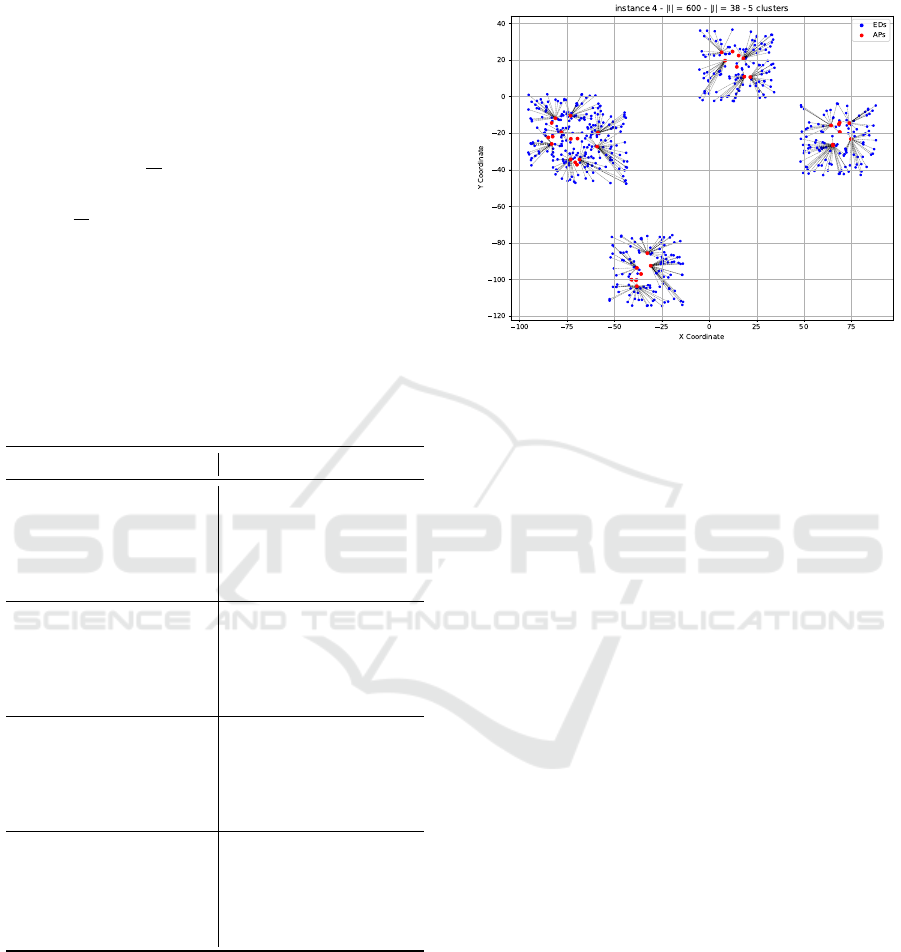
In the first set of instances (1 to 5), the APs and
EDs coordinates are distributed across 5 clusters. The
values of |I| vary between 100 and 800, and the val-
ues of |J| vary between 20 and 40. As illustrated in
Figure 3, EDs coordinates can deviate more signifi-
cantly than APs from the cluster’s origin points C
h
,
(r
(ED)
max
≥ r
(AP)
max
). With this configuration, peripheral
APs tend to demonstrate a higher likelihood of reac-
tivation compared to centrally located APs. This can
be attributed to their proximity to EDs, which reduces
the values of the solutions by minimizing the overall
distances between APs and EDs.
Figure 3: Result of instance 4 (peripheral APs selection).
In the second set of instances (6 to 10), the number
of EDs is fixed at 500 and the number of APs is set to
20, while the number of clusters varies between 2 and
6. With this increase in the number of clusters, the
number of selected APs |P| also increases. This can
be attributed to the distances between clusters, where
the placement of additional APs in the clusters tends
to reduce the overall cost in the objective function,
compared to placing fewer APs and covering longer
distances across clusters.
In the third set of instances (11 to 15), the number
of disconnected APs matches the number of clusters.
The resulting CVRP instances are thus no longer clus-
tered, since this configuration enforces that generally
at most one AP would be selected per cluster. We ob-
serve from Table 2 that |P| does not match exactly |H|
for all the instances. Indeed, in instances 11 and 15,
|P| = |H| − 1. This can be attributed to the overlap of
clusters in these two instances (see Figure 4).
In the fourth set of instances (16 to 20), the num-
ber |I| of EDs is significantly higher compared to the
preceding sets. This increase led to a significant in-
crease in the CPU time required for solving these in-
stances compared to the previous sets, especially for
instances 18, 19 and 20 where |J| is relatively high
compared to 16 and 17. However, these instances re-
mained solvable within one minute.
4.3.2 Phase II: UAVs Path Planning
As previously discussed, we investigate two scenar-
ios: one in which the UAV depot is positioned pe-
ripherally in a safe zone outside the disaster area, and
another where the depot is centrally located within the
Optimal Covering and Trajectory Planning for Air-Ground Integrated Networks in Post-Disaster Scenarios
315

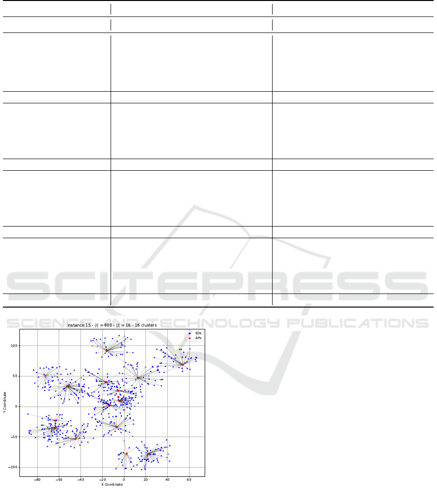
Table 3: Computational results of the CVRP.
instance Centered Depot Peripheral Depot
inst |K| |P| Q Tgh init VNS CPX
II
CPU(s) gap init VNS CPX
II
CPU(s) gap
1 2 10 71 0.85 506 506 506 0.19 0.00 1403 1403 1401 0.30 0.14
2 2 20 192 0.85 492 481 480 126.45 0.20 1735 1714 1714 941.08 0.00
3 2 20 178 0.85 583 574 565 14.32 1.59 2002 1990 1978 39.17 0.60
4 2 22 225 0.85 438 416 416 61.27 0.00 1285 1265 1265 3600 0.00
5 2 22 219 0.85 496 490 490 3600 0.00 1857 1837 1837 3600 0.00
avg. 0.35 avg. 0.14
6 2 11 123 0.90 304 304 300 1.15 1.33 1539 1539 1538 1.53 0.06
7 2 12 103 0.90 386 386 376 2.67 2.65 1796 1796 1787 1.88 0.50
8 2 13 115 0.90 275 275 270 1.70 1.85 1345 1342 1337 1.96 0.37
9 2 14 122 0.90 426 426 398 1.02 7.03 1762 1762 1734 87.52 1.61
10 2 16 140 0.90 169 158 143 0.13 10.48 1484 1474 1469 117.66 0.34
avg. 4.66 avg. 0.57
11 2 11 85 0.92 431 431 416 0.29 3.60 1668 1668 1666 0.74 0.12
12 2 13 122 0.92 453 453 442 54.96 2.48 1850 1850 1839 281.34 0.59
13 2 14 101 0.92 328 328 315 245.19 4.12 1279 1279 1264 1.89 1.18
14 2 15 116 0.92 495 495 495 2.35 0.00 1641 1640 1636 1.51 0.24
15 2 15 96 0.92 298 298 290 1.71 2.75 1429 1429 1428 1.68 0.07
avg. 2.59 avg. 0.44
16 2 14 131 0.88 389 389 389 16.09 0.00 1353 1353 1312 0.56 3.12
17 2 17 186 0.88 454 451 446 66.48 1.12 1742 1737 1732 925.90 0.28
18 2 23 203 0.88 505 495 480 3600 3.12 1750 1740 1739 2972.61 0.05
19 2 24 203 0.88 608 587 587 2920.41 0.00 1077 1059 1059 151.50 0.00
20 2 25 245 0.88 487 476 473 3600 0.63 1761 1745 1745 203.42 0.00
avg. 0.97 avg. 0.69
Figure 4: Result of instance 15 (neighboring clusters).
disaster zone. For the studied instances, the tightness
ranges between 0.85 and 0.92 (see equation (17)) and
the number of UAVs |K| is set to 2. The maximum
number of APs to be reactivated |P| is 25. To evaluate
our VNS on larger instances, we use five well-known
CVRPLIB benchmarks (see Appendix).
The results in Table 3 show that the proposed
method can find high quality solutions in most of the
instances. For 25 out of the 40 studied instances, the
gap is less than 1% and the optimal values were ob-
tained using our method for 11 instances among them.
Clearly, the solutions obtained for the instances hav-
ing a central depot are significantly less than those
having a peripheral depot. This can be explained by
the fact that the UAVs must travel additional distances
from a depot located in a safe area at the coordinates (-
250, -250) to reach the disaster area. In contrast, with
a central depot, the UAVs begin their journey from a
charging station located at the center of the disaster
area at coordinates (0, 0).
In the first set of instances (1 to 5), the tightness
is set to 0.85. For both centered and peripheral depot
configurations, the gap is less than 2% for the ten in-
stances, and is equal to 0% for six out of them. In the
second set of instances (6 to 10), we increase the tight-
ness to 0.90. The average gap compared to CPLEX
is 4.66% for centered depots and is equal to 0.57%
for peripheral depots. Note that the solution returned
by CPLEX for instance 10 (centered depot) is rela-
tively low compared to instances 6, 7, 8 and 9. This
is highly related to the structure of the instance. As
ICORES 2025 - 14th International Conference on Operations Research and Enterprise Systems
316

illustrated in Figure 4, this instance contains several
neighboring clusters. Thus the UAVs will not have to
move large distances between them. Moreover, these
clusters are centrally located around the UAVs depot
located at coordinates (0, 0) which significantly re-
duces the total traveled distance by UAVs. In the third
set of instances (11 to 15), the tightness is set to 0.92.
The average gap compared to CPLEX is 2.59% for
centered depots, and is 0.44% for peripheral depots.
Moreover, for 5 out of the 10 instances, the instance
gap is less than 1%. In the fourth set of instances (16
to 20), the average gap is 0.97% for centered depots
and is equal to 0.69% for peripheral depots.
5 CONCLUDING REMARKS
In this paper we study the use of UAVs to recon-
nect deactivated APs in post-disaster scenarios. We
propose a two-phase reactivation strategy. First we
present a UCFLP formulation to select the best APs to
be reactivated, then we solve it using CPLEX. The ob-
jective function minimizes the total distances between
EDs and APs as well as the UAVs battery reactivation
costs. Second, we present a CVRP formulation for
the UAVs path planning to reactivate the selected APs
in phase I. The objective function minimizes the total
traveled distance by UAVs. We devise a VNS meta-
heuristic to solve it and we compare its solutions to
the ones returned by CPLEX solver. Experimental re-
sults show that the proposed method performs well
compared to CPLEX within just a one-minute time
limit.
The studied problem can be formulated otherwise
by considering different constraints. For the first
phase, it would be interesting to explore other pos-
sible scenarios for the EDs covering problem. For
instance, in the case where an ED can be served by
more than one AP, a capacitated facility location prob-
lem formulation might be more suitable than UCFLP.
In scenarios where the number of APs to be reacti-
vated is limited, the capacitated maximum cover loca-
tion problem might be more suitable for selecting the
most crucial APs in order to maximize the EDs cov-
ering. In situations where minimizing the maximum
distance between EDs and the nearest APs that can
serve them is a priority, a capacitated p-center prob-
lem formulation can be beneficial. In scenarios where
enhancing the overall efficiency is a priority, a capac-
itated p-median problem formulation can be useful.
For the second phase, exploring different data point
distribution patterns, including both clustered and dis-
persed configurations, could also be valuable. An-
other consideration that might be useful involves the
assignment of weights to EDs or APs. For instance,
prioritizing geographically distant EDs or APs from
hospitals and emergency response units may be use-
ful to improve the overall response efficiency.
REFERENCES
Adsanver, B., Coban, E., and Balcik, B. (2024). A
predictive multistage postdisaster damage assessment
framework for drone routing. International Transac-
tions in Operational Research.
Augerat, P., Belenguer, J. M., Benavent, E., Corber
´
an,
´
A.,
Naddef, D., and Rinaldi, G. (1995). Computational
results with a branch and cut code for the capacitated
vehicle routing problem.
Calamoneri, T., Cor
`
o, F., and Mancini, S. (2024). Manage-
ment of a post-disaster emergency scenario through
unmanned aerial vehicles: Multi-depot multi-trip ve-
hicle routing with total completion time minimization.
Expert Systems with Applications, 251:123766.
Chowdhury, S., Shahvari, O., Marufuzzaman, M., Li, X.,
and Bian, L. (2021). Drone routing and optimization
for post-disaster inspection. Computers & Industrial
Engineering, 159:107495.
Clarke, G. and Wright, J. W. (1964). Scheduling of vehicles
from a central depot to a number of delivery points.
Oper. Res., 12(4):568–581.
Coco, A., Duhamel, C., Santos, A., and Haddad, M.
(2024). Solving the probabilistic drone routing prob-
lem: Searching for victims in the aftermath of disas-
ters. Networks, 84.
CPLEX (2024). IBM ILOG CPLEX Optimization Studio.
Accessed: 2024-09-16.
Desrochers, M. and Laporte, G. (1991). Improvements
and extensions to the miller-tucker-zemlin subtour
elimination constraints. Operations Research Letters,
10(1):27–36.
Fisher, M. L. (1994). Optimal solution of vehicle rout-
ing problems using minimum k-trees. Operations Re-
search, 42(4):626–642.
Holmberg, K., R
¨
onnqvist, M., and Yuan, D. (1999). An ex-
act algorithm for the capacitated facility location prob-
lems with single sourcing. European Journal of Op-
erational Research, 113(3):544–559.
Mladenovic, N. (2004). A tutorial on variable neighborhood
search.
Mladenovi
´
c, N. and Hansen, P. (1997). Variable neighbor-
hood search. Comput. Oper. Res., 24(11):1097–1100.
Uchoa, E., Pecin, D., Pessoa, A., Poggi, M., Vidal, T., and
Subramanian, A. (2016). New benchmark instances
for the capacitated vehicle routing problem. European
Journal of Operational Research, 257.
Yucesoy, E., Balcik, B., and Coban, E. (2024). The role
of drones in disaster response: A literature review of
operations research applications. International Trans-
actions in Operational Research.
Optimal Covering and Trajectory Planning for Air-Ground Integrated Networks in Post-Disaster Scenarios
317

APPENDIX
To evaluate the efficiency of our VNS, we use five
well-known benchmarks from CVRPLIB. Three from
these benchmarks are from (Augerat et al., 1995), re-
ferred to as A, B and P respectively. The fourth bench-
mark is taken from (Fisher, 1994), referred to as F.
The remaining benchmark is taken from (Uchoa et al.,
2016), referred to as X. The instances include con-
straints on the vehicles capacity and on the number
of vehicles. Given that our resolution procedure does
not impose any constraints on the number of vehicles,
we only consider instances where the number of ve-
hicles in our initial solution algorithm aligns with the
vehicle number constraints established by the bench-
marks. All instances adhere to a naming convention
such as A-n32-k5, where n32 refers to 31 client nodes
along with a single depot, and k5 denotes the use of
five vehicles. These instances include various con-
figurations. In what follows, we give more details on
these configurations, we present the computational re-
sults obtained by running the VNS on these instances,
and we compare them to the solutions provided in
CVRPLIB.
In set A, the client nodes are uniformly dis-
tributed, whereas in set B, they are organized into
clusters, with the depot sometimes not centrally lo-
cated. The tightness of the studied instances from
A ranges between 0.81 and 0.96. For B instances,
the tightness ranges between 0.82 and 0.97. Set F
contains two instances with tightness values 0.90 and
0.95. These represent real data taken from a day
of grocery deliveries from the Peterboro of National
Grocers Limited. In set P, the instances are uniformly
distributed and the tightness of the studied instances
ranges between 0.88 and 0.97. For benchmarks A, B,
P and F the number of client nodes ranges between 19
and 135. In order to evaluate the performance of our
VNS on larger instances, we use the set X. In the ex-
amined X instances, the vehicle count varies between
6 and 131, and the number of customers ranges from
106 to 856. Note that for this set, we only consider
instances where the optimal solutions are provided in
CVRPLIB.
For set A, our method deviates from the optimal
solutions by 3.03% on average and the gap is less than
3% in 11 out of the 21 instances. For set B, the av-
erage gap is 1.62% and in 11 out of the 16 instances,
the gap is less or equal than 2%. For set F, the average
gap is 1.22%. The average gap for set P is 8.37% and
is 5.22% for set X.
The proposed resolution procedure has generally
demonstrated robustness across various configuration
changes, including both central and peripheral depot
placements, as well as instances involving clustered
data points, uniform distributions, and hybrid ones.
The method performed well across a range of tight-
ness levels. However, we observe that in some in-
stances of uniform distributions in P, the gap reached
18.00%. In X, the gap reached 10.29%. In contrast,
the clustered configurations in B consistently yielded
strong performance. These findings suggest that fur-
ther refinement of the VNS neighborhoods could en-
hance its applicability to scenarios with uniformly
distributed and hybrid configurations of client loca-
tions.
ICORES 2025 - 14th International Conference on Operations Research and Enterprise Systems
318

Table 4: Computational results of the VNS on CVRPLIB
instances.
instance initial VNS optimal gap
solution (%)
A-n32-k5 847 827 784 5.48
A-n33-k5 693 675 661 2.11
A-n33-k6 745 743 742 0.13
A-n34-k5 793 793 778 1.92
A-n36-k5 829 805 799 0.75
A-n37-k5 697 690 669 3.13
A-n37-k6 993 984 949 3.68
A-n39-k5 900 889 822 8.15
A-n39-k6 878 846 831 1.80
A-n44-k6 1018 987 937 5.33
A-n45-k7 1205 1195 1146 4.27
A-n46-k7 940 932 914 1.96
A-n48-k7 1104 1096 1073 2.14
A-n54-k7 1174 1172 1167 0.42
A-n55-k9 1113 1108 1073 3.26
A-n60-k9 1373 1365 1354 0.81
A-n62-k8 1362 1339 1288 3.95
A-n63-k10 1378 1363 1314 3.72
A-n64-k9 1452 1437 1401 2.56
A-n69-k9 1203 1185 1159 2.24
A-n80-k10 1870 1866 1763 5.84
avg. 3.03
B-n31-k5 681 676 672 0.59
B-n34-k5 806 789 788 0.12
B-n35-k5 976 966 955 1.15
B-n38-k6 834 819 805 1.73
B-n39-k5 566 560 549 2.00
B-n43-k6 757 749 742 0.94
B-n44-k7 936 926 909 1.87
B-n45-k5 756 756 751 0.66
B-n50-k7 748 743 741 0.26
B-n50-k8 1395 1328 1312 1.21
B-n52-k7 760 756 747 1.20
B-n56-k7 738 725 707 2.54
B-n57-k9 1658 1638 1598 2.50
B-n63-k10 1608 1568 1496 4.81
B-n68-k9 1310 1299 1272 2.12
B-n78-k10 1266 1250 1221 2.37
avg. 1.62
F-n45-k4 739 725 724 0.13
F-n135-k7 1200 1189 1162 2.32
avg. 1.22
Table 5: Computational results of the VNS on CVRPLIB
instances.
instance initial VNS optimal gap
solution (%)
P-n19-k2 240 240 212 13.20
P-n20-k2 249 249 216 15.27
P-n21-k2 249 249 211 18.00
P-n22-k2 253 253 216 17.12
P-n40-k5 505 471 458 2.83
P-n45-k5 534 528 510 3.52
P-n50-k7 582 582 554 5.05
P-n55-k7 620 604 568 6.33
P-n55-k10 730 725 694 4.46
P-n60-k10 794 792 744 6.45
P-n65-k10 840 838 792 5.80
P-n76-k4 663 647 593 9.10
P-n101-k4 731 693 681 1.76
avg. 8.37
X-n106-k14 27997 27848 26362 5.63
X-n110-k13 15920 15916 14971 6.31
X-n120-k6 14638 14117 13332 5.88
X-n129-k18 29954 29801 28940 2.97
X-n143-k7 17714 17317 15700 10.29
X-n157-k13 18026 18026 16876 6.81
X-n162-k11 15156 15042 14138 6.39
X-n167-k10 22014 21577 20557 4.96
X-n181-k23 26615 26463 25569 3.49
X-n186-k15 25604 25491 24145 5.57
X-n190-k8 17805 17561 16980 3.42
X-n204-k19 21442 21185 19565 8.28
X-n209-k16 32242 31797 30656 3.72
X-n219-k73 118364 118364 117595 0.65
X-n237-k14 29786 29505 27042 9.10
X-n251-k28 41145 41145 38684 6.36
X-n261-k13 28911 28371 26558 6.82
X-n275-k28 22447 22376 21245 5.32
X-n284-k15 22057 21855 20215 8.11
X-n317-k53 79492 79492 78355 1.45
X-n331-k15 33423 33182 31102 6.68
X-n367-k17 24745 24547 22814 7.59
X-n376-k94 149181 149181 147713 0.99
X-n439-k37 38675 38490 36391 5.76
X-n548-k50 89574 89429 86700 3.14
X-n655-k131 108353 108353 106780 1.47
X-n856-k95 92368 92368 88965 3.82
avg. 5.22
Optimal Covering and Trajectory Planning for Air-Ground Integrated Networks in Post-Disaster Scenarios
319