Comparison Between CNN and GNN Pipelines for Analysing the Brain

in Development

Antoine Bourlier

1,2

, Elodie Chaillou

, Jean-Yves Ramel

and Mohamed Slimane

LIFAT, Universit

e de Tours, 64 Av. Jean Portalis, Tours, France

INRAe, CNRS, Universit

e de Tours, Nouzilly, France

LISTIC, Universit

e de Savoie Mont-Blanc, Chamb

ery, France

Keywords:

Graph, Machine Learning, MRI, Segmentation.

Abstract:

In this study, we present a new pipeline designed for the analysis and comparison of non-conventional animal

brain models, such as sheep, without relying on neuroanatomical priors. This innovative approach combines

an automatic MRI segmentation with graph neural networks (GNNs) to overcome the limitations of traditional

methods. Conventional tools often depend on predeﬁned anatomical atlases and are typically limited in their

ability to adapt to the unique characteristics of developing brains or non-conventional animal models. By

generating regions of interest directly from MR images and constructing a graph representation of the brain,

our method eliminates biases associated with predeﬁned templates. Our results show that the GNN-based

pipeline is more efﬁcient in terms of accuracy for an age prediction task (63.22%) compared to a classical

CNN architecture (59.77%). GNNs offer notable advantages, including improved interpretability and the

ability to model complex relational structures within brain data. Overall, our approach provides a promising

solution for unbiased, adaptable, and interpretable analysis of brain MRIs, particularly for developing brains

and non-conventional animal models.

1 INTRODUCTION

Automated methods have facilitated brain MRI anal-

ysis, especially in humans and conventional animal

models (Kaur and Gaba, 2021; Park and Friston,

2013). However, such tools are rarely available to

study developing brains or non-conventional animal

models like sheep. In these cases, brain structures

identiﬁcation is often manual or based on automatic

segmentation using signal intensity and templates,

when available (Nitzsche et al., 2015; Ella et al.,

2017). These methods depend on biological priors

and the accuracy of atlases, which may not fully cap-

ture individual variations or patterns associated to dif-

ferent brain disorders. These issues are especially

challenging for developing brains, where contrast is

weak, development is uneven, and some structures are

not visible (Li et al., 2019). Additionally, using pre-

deﬁned regions may limit the discovery of new brain

correlates.

To address segmentation bias, convolutional neu-

ral networks (CNNs) have been introduced, as they

work directly on MR images without segmentation

(Srinivasan et al., 2024; Coupeau et al., 2022). CNNs

provide valuable whole-brain or abnormality-level in-

formation but require large labelled datasets to learn

low-level image features for classiﬁcation or segmen-

tation tasks. This makes them unsuitable for the de-

veloping brain or non-conventional animal models

with small cohorts.

In this paper, we present a pipeline to address

both segmentation biases and CNN limitations. We

propose generating regions of interest (ROIs) with-

out relying on neuro-anatomical priors. We use voxel

intensities to create segmented images via 2 differ-

ent segmentation algorithms. Additionally, we use

graph neural networks (GNNs) to identify and anal-

yse anatomical patterns, as GNNs model the brain as

interconnected patches, capturing complex relation-

ships between regions (Cui et al., 2021; Li et al.,

2021; Ravinder et al., 2023). By avoiding prede-

ﬁned atlases, our method allows more ﬂexible, image-

driven exploration of the brain. This approach is par-

ticularly useful for studying non-conventional animal

models of brain development, such as sheep. It offers

the potential to discover new structures and patterns

in both human and animal studies, enhancing under-

Bourlier, A., Chaillou, E., Ramel, J.-Y. and Slimane, M.

Comparison Between CNN and GNN Pipelines for Analysing the Brain in Development.

DOI: 10.5220/0013173500003912

Paper published under CC license (CC BY-NC-ND 4.0)

In Proceedings of the 20th International Joint Conference on Computer Vision, Imaging and Computer Graphics Theory and Applications (VISIGRAPP 2025) - Volume 3: VISAPP, pages

475-482

ISBN: 978-989-758-728-3; ISSN: 2184-4321

475

standing and improving the diagnosis and treatment

of developing brain disorders.

This paper focuses on the speciﬁc task related to

study the developing brain. We tested various GNN

architectures and compared them to a classical CNN

approach. The comparison addresses the challenge of

predicting brain age in non-conventional animal mod-

els without neuro-anatomical priors. The next sec-

tions discuss the limitations of classical brain MRI

processing methods to study developing brain disor-

ders and non-conventional animal models. We de-

tail our pipeline, including segmentation, graph gen-

eration, and GNN prediction. Then, we present the

experimental comparison with a CNN approach, fol-

lowed by a discussion of its advantages and limita-

tions.

2 RELATED WORKS

2.1 Classical Approaches Used on Brain

MRI

The 2 main tasks studied in the literature are im-

age/brain segmentation (Coupeau et al., 2022) and

image/brain classiﬁcation (Srinivasan et al., 2024;

Kaur and Gaba, 2021; Poriya, 2023). In both cases,

machine learning algorithms provide powerful tools

such as CNN and graph convolutional network (GCN)

layers that compute and ﬁnd on its own the most rele-

vant features. Whether CNN or GNN is chosen, both

require speciﬁc key such as pre-processing and patch

extraction. The aim of the MRI pre-processing (de-

noising, normalisation etc.) is to adjust the inten-

sity values of the images to a standard range in or-

der to ensure consistency. A resampling step is used

to align images to a common voxel size or resolution

and a registration step can be added to align images

to a standard anatomical space, often using a template

brain. To remove non-brain tissues (e.g., skull, scalp)

cropping and skull-stripping are performed on MRI

images.

2.1.1 Segmentation

The aim of segmentation is to delineate and identify

anatomic ROI in the brain MRI, segmented images

being used to create a graph representation. Segmen-

tation is performed manually or using atlases based

on individual brain images or templates (Van Essen

and Drury, 1997; Yang et al., 2020; Fil et al., 2021).

They are used for ROI identiﬁcation, delineating vari-

ous regions and structures or serve as reference points

to align individual MRI scans to a common space, fa-

cilitating consistent and accurate analysis across sub-

jects.

2.1.2 CNN Design

A CNN typically consists of multiple layers, includ-

ing convolutional layers, pooling layers, and fully

connected layers. Using advanced CNN architec-

tures, such as AlexNet (Krizhevsky et al., 2012), or

ResNet (He et al., 2016), enhances the model’s abil-

ity to learn complex patterns and achieve high per-

formance in various MRI analysis tasks, including

classiﬁcation, clustering etc. Incorporating biologi-

cal priors through brain atlases can further reﬁne these

methods, offering improved accuracy and consistency

in brain MRI analysis. Concerning brain age predic-

tion, several CNN architectures have been proposed

including VGG, ResNet, and DenseNet (Cole et al.,

2017; Jiang et al., 2020).. More advanced CNN archi-

tectures including attention mechanisms have since

been developed to boost the representational power

and improve prediction accuracy (Lam et al., 2020;

Cheng et al., 2021).

2.1.3 Graph Design

Nodes of a graph are usually deﬁned at a region level

(i.e., one node per brain structure). The way the re-

gions are chosen is really linked with the aim of the

study and could represent neurons, anatomical struc-

tures, brain tissues, voxels, etc. From an anatomi-

cal point of view, node features provide information

about the position of the region (coordinates of the

center of gravity, orientation etc.), the shape (volume,

sphericity etc.), the signal intensity, which is useful to

understand the composition of the tissue, etc. Graph

theory features can also be used (centrality, strength

etc.). Several ways exist to build the edges of the

graph and characterise them depending on the aim of

the study. Generally, three types of edges are distin-

guished: structural, functional, and effective connec-

tions (Fedorov et al., 2012). The possibilities for edge

features are also numerous: Euclidean distances, tract

lengths, connection costs, etc. (Bullmore and Bassett,

2011; Sporns, 2018). Possibly, the trickiest compo-

nent in creating the brain network lies in edge cre-

ation. We could create a fully connected graph but for

an interpretable and efﬁcient representation, we aim

to reduce the edge density, so that only the signiﬁcant

connections are displayed. This is achieved by intro-

ducing a threshold and removing edges that do not

meet the required criteria. How to deﬁne the threshold

is still an active research question: typical approaches

use customised, statistical, or expert-based criteria.

VISAPP 2025 - 20th International Conference on Computer Vision Theory and Applications

476

2.1.4 GNN Design

Once the brain has been modelled as a graph, GNNs

are trained to analyse these graphs, and to capture

complex relationships and variations in brain organ-

isation (Li et al., 2021; Ravinder et al., 2023; Srini-

vasan et al., 2024; Coupeau et al., 2022). For age

prediction, GNN architectures have also been pro-

posed to better exploit the inter-region relationships

like a GNN architecture that processes diffusion-

MRI-derived brain connectivity data while consider-

ing brain network topological locality (Sporns, 2007).

Many methods like multi-hop graph attention or

graph Transformer framework require graph struc-

tures such as tractography networks or the registra-

tion of multi-modal images based on a standard brain

template (Lim et al., 2024; Cai et al., 2023).

2.2 Approaches for Brain in

Development and Non-Conventional

Animal Model

The analysis of brains in development and/or from

non-conventional animal models, rises several chal-

lenges and considerations that differ from the analy-

sis of adult human brains. The primary differences in-

clude anatomical variations, the lack of standardised

atlases, tools and often smaller datasets.

For example, brain segmentation of non-conventional

animal models is often done manually. This pro-

cess is time-consuming, requires neuro-anatomical

expertise and introduces a high level of bias due

to inter-individual variation between operators (Fe-

dorov et al., 2012). An alternative to the manual

segmentation, is the atlas-based registration method.

The concept involves creating a template, achieved

by registering and normalising multiple brain MR

images into a common space using afﬁne transfor-

mations, followed by segmentation of the template

and transferring the segmentation to each MR image

(De Vico Fallani et al., 2017). While this method is

beneﬁcial for segmenting numerous images simulta-

neously, post-processing is essential to ensure accu-

rate correspondence between the segmentation and in-

dividual anatomy.

There are also some automatic and incremental seg-

mentation algorithms available that incorporate bio-

logical priors (Galisot et al., 2022).

3 THE PROPOSED PIPELINE

3.1 From 3D MR Images to Graphs

We propose a generic pipeline for transforming

3D MR images of brains in development of non-

conventional animal models into graphs. The objec-

tive is to generate graphs incorporating a maximum of

information from the brains and, to let the GNN select

the useful information inside these graphs (Figure 1).

3.2 Pre-Processing

Pre-processing includes skull-stripping and z-score

normalisation. Z-score normalisation is reported to be

more suitable for brain MRI analysis, particularly in

machine learning, because it maintains the alignment

of intensity peaks for white matter, grey matter, and

CSF (Schmid, 2023). After the image pre-processing,

the graph creation is divided into two parts: node cre-

ation and edge creation.

3.3 Nodes and Edges Creation

The creation of nodes corresponds to segmented ROIs

(Figure 2). Since our goal is to process brains in de-

velopment of growing non-conventional animal mod-

els, segmentation without biological priors offers an

alternative approach to analyse brain MR images and

constructing graphs. This method relies solely on im-

age information and the data is treated purely as a

conventional image rather than speciﬁcally as a brain

image. For this study, we have chosen to test a

histogram-based clustering algorithm and a ”split and

merge” algorithm. The histogram-based algorithm

splits the intensity range into N equal parts. One of

the main challenges is to determine the optimal pa-

rameters of the algorithm which depends on the study

objectives, the desired level of details etc. In the im-

age 1, the ﬁrst segmentation is made with this algo-

rithm. The second algorithm is the ”split and merge”

algorithm, (Gonzalez and Woods, 2017) which oper-

ates in two distinct phases: ”split” and ”merge”. In the

ﬁrst phase, the algorithm recursively divides the im-

age into smaller and homogeneous regions (”cubes”)

based on a user-deﬁned homogeneity criterion and a

minimum region size. The homogeneity criterion is

the intensity amplitude of the region intensities. Then,

in the merge step, adjacent regions are combined if

their merged region meets another homogeneity crite-

rion. Each region of the segmentation is represented

as a node with associated normalised features : re-

gion’s volume divided by the brain’s volume, region’s

surface area divided by the brain’s surface area, mean

Comparison Between CNN and GNN Pipelines for Analysing the Brain in Development

477

Figure 1: Graph construction pipeline in which we tested different segmentation algorithms (histogram-based segmentation

and ”Split and merge” segmentation) and parameters. ”N” is the hyperparameter of the histogram-based algorithm. ”Split” and

”merge” are the hyperparameters of the ”split and merge” algorithm. ”p” is the number of edge features, 0 in our experiment.

intensity of the voxels inside the region, standard de-

viation of the intensity, region’s center of gravity in

the spherical coordinate system (radial distance from

the center of gravity of the brain, polar angle and az-

imuthal angle).

Then, there are many possibilities to deﬁne the

edges, and we propose to build an adjacency graph

by connecting two nodes if the geometric distance be-

tween them is below a threshold d (d is a hyperparam-

eter of the method). Depending on the task the user

wants to perform with the graphs, choosing the appro-

priate value for d might be another challenge.

3.4 Graph Analysis and Classiﬁcation

As discussed before, GNNs are particularly well-

suited for brain MRI analysis due to their ability to

capture the intricate relationships between different

brain ROIs. Unlike CNNs, which primarily focus on

local voxel information, GNNs can model the brain at

a higher level where nodes represent different struc-

tures or parts of structures and edges represent con-

nections between them. This relational representation

can lead to more accurate and interpretable predic-

tions.

In the conducted experiments, the proposed GNN ar-

chitecture tries to harness these advantages to predict

the age of a sheep brain (by solving a graph classiﬁ-

cation task with K classes of age range) (Figure 2).

3.4.1 Graph Convolution Layers

To propagate the information over the graph, we use

a set of 3 convolution layers. As described in the pre-

vious sections, multiple convolution layers are avail-

able. Our dataset is relatively small, consisting of ap-

proximately 200 graphs. Consequently, using a com-

plex neural network with sophisticated and large lay-

ers is not advisable. Therefore, in this study, we

utilised the GCNConv layer, which considers both the

node feature (F) and adjacency (A) matrices. The GC-

NConv layer computes updated node features by ag-

gregating information from neighbour nodes and their

connections. The input to the ﬁrst layer consists of the

node features matrix (F), initialized with 7 features

per node, and the adjacency matrix (A) that encodes

the graph structure. The transformation from 7 fea-

tures to 32 or 64 features occurs progressively across

the layers, as follows:

• First set of parameters: The model begins by

transforming the 7 initial features into 8 features

using the ﬁrst GCNConv layer (Figure 2). This

output is then passed to a second GCNConv layer,

which further transforms it to 16 features. Finally,

a third GCNConv layer transforms the features to

32 dimensions. Each layer applies a learned linear

transformation followed by an activation function

(ReLU in our case), enabling the network to pro-

gressively capture complex patterns in the data.

• Second set of parameters: Instead of incremental

changes, the model starts with 7 features and dou-

bles the number of dimensions at each layer: from

7 to 16, then to 32, and ﬁnally to 64. This more

aggressive dimensionality increase aims to test the

model’s ability to learn richer representations.

Dropout regularisation is applied and set to 0.5 to pre-

vent overﬁtting during training.

3.4.2 Pooling and Fully Connected Layers

A global mean pooling and a global max pooling were

tested to capture interesting information while taking

into account the small amount of data.

The pooled features are then passed through three

fully connected (FC) layers (fc1, fc2 and fc3) to per-

form the classiﬁcation. The ﬁrst FC layer maps the

features to a 128-dimensional space, the second FC

VISAPP 2025 - 20th International Conference on Computer Vision Theory and Applications

478

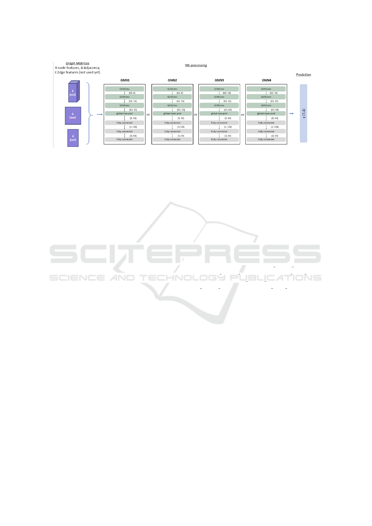
Figure 2: different GNN architectures according to the number of convolutions and the type of readout pooling have been

evaluated for the different types of generated graphs presented in Figure 1.

layer to a 64-dimensional space and the third FC layer

reduces this to a 7-dimensional space, to match with

the (K)=7 age classes of the sheep brain.

In total, we have tested 4 different architectures

by combining the 2 sets of convolution parameters

and the 2 global poolings (GNN1, GNN2, GNN3 and

GNN4, (Figure 2)).

4 EXPERIMENTS AND RESULTS

We conducted experiments with different CNN and

GNN architectures to analyse which ones are the best

suited to predict the age of brains of non-conventional

animal models such as sheep. The experiments were

conducted on a machine equipped with an Intel Core

i7-11850H CPU running at 2.50 GHz, 32 GB of

RAM, and an NVIDIA GeForce RTX A3000 Laptop

GPU. All computations were performed using Python

3.11.8 with Pytorch 2.2.2+cu121 frameworks. This

section describes the used datasets and protocols.

4.1 Datasets, Protocol and Metric

Description

4.1.1 Datasets

The dataset used is composed of 195 3D-T1w-MRI

from different projects which were all conduct in

”Ile de France” growing and adult sheep from the

“Unit

e Exp

erimentale de Physiologie Animale de

l’Orfrasi

ere” (UEPAO, INRAE Val de Loire, France;

https://doi.org/10.15454/1.5573896321728955E12).

MRI were acquired in vivo with a 3 Teslas Siemens

Magnetom Verio® scanner (Erlangen, Germany)

located at the imaging platform PIXANIM. A 4-

channel Siemens FLEX coil was used. T1-weighted

images were acquired with the 3D-MPRAGE se-

quence with 2 or 4 numbers of excitations according

to the project. The plane resolution of the T1-w

MRI was between 0.4x0.4mm and 0.5x0.5mm. We

created 5 segmentations for each MRI in total : 3

from our histogram-based algorithm and 2 from

our split and merge algorithm. The parameter of

histogram-based algorithm is set to N=6, N=20 and

N=30. N=6 gives a segmentation similar to a tissue

segmentation (White matter, gray matter and CSF).

The other parameters produced visually interesting

results, maximizing the expressiveness of the image

content while ensuring that the segmentation remains

clear and not overly noisy. After testing different set

of parameters we chose 2 sets of parameters for the

split and merge : {homogeneity during split=10, ho-

mogeneity during merge=40, minimal cube size=1}

and {homogeneity during split=20, homogene-

ity during merge=60, minimal cube size=1}. Each

segmentation are then transformed into an adjacency

graph (distance threshold d=0) with every attribute

described previously.

4.1.2 Protocol and Metrics

During our experiments, we try to learn and predict

the age of the subjects. Age prediction can be a hard

task regarding our data. That’s why we decided to

learn a classiﬁcation task instead of a regression task,

the latter considered as more difﬁcult to perform. We

decided to distribute the images into K=7 classes of

ages (Table 1) in order to obtain balanced with enough

representative images into each class. The ranges as-

sociated with each class have been deﬁned based on

available data, corresponding to 10 to 20 days (with

no data available for the range between 70 to 120

days).

The proposed pipelines based on GNN architec-

tures were compared with a classical CNN architec-

ture working with low level image features (Figure

3). In the following we compare our pipeline with the

CNN architecture that presented the best results after

Comparison Between CNN and GNN Pipelines for Analysing the Brain in Development

479

Table 1: Organization of the 7 classes according to the range of age (days) and number of subjects per class.

Class 1 2 3 4 5 6 7

Age (days) 0-10 11-20 21-30 31-40 41-50 51-70 123-139

Numbers 33 16 22 24 61 24 15

Figure 3: Optimized CCN pipeline. The architecture con-

tains 2 convolution layers (Conv3d), a ﬂattening layer and

3 linear layers.

learning with different layer numbers and sizes. The

CNN consists of a 3D convolution layer with a kernel

size of 3x3x3, followed by a 3D max-pooling layer of

size 2x2. This sequence of convolution and pooling

layers is repeated once. The output is then ﬂattened

into a vector, which is passed through three fully con-

nected layers that progressively reduce its size to 128,

64, and ﬁnally 7 dimensions.

The 195 images (see dataset section) were used to

create the training (50% of the MR-images), the vali-

dation (25% of the MR-images) and the test datasets

(25% of the MR-images). We carefully design the

test dataset to be representative of all the data by bal-

ancing the classes and projects to remove any project

bias. We performed a shufﬂe split validation which is

well suited for small datasets. The training lasts 300

epochs. The loss function is the cross-entropy loss

with a learning rate of 0.001.

4.2 Results

In terms of accuracy, the GNN pipeline remains bet-

ter than a classical CNN pipeline with an average ac-

curacy of 63.22% compared to 59.77% for the CNN

(table 2). These results show that our pipeline could

be convenient for a classical task like age prediction.

The split and merge pipelines seem to perform bet-

ter than the histogram-based pipelines achieving an

average accuracy of 51.43% compared to 37.73%.

This could be explained by the fact that the number

of nodes is not ﬁxed and could be discriminative be-

tween the classes. For example, we found that class 6

has an average of 1,110 nodes, compared to 2,205 for

class 7, making it very easy to discriminate between

them.

Concerning the GNN architecture, the GNN with

global better results was the GNN4 with a conv1=16,

conv2=32, conv3=64 and a global mean pooling with

an average accuracy of 45.08%. The other architec-

tures have the following average accuracies : GNN1

= 43.49%, GNN2 = 40.48% and GNN3 = 43.81%.

These results suggest that the global max pooling is a

little bit better in average. Other pooling methods and

architectures need to be experimented.

We calculated the confusion matrix of each training

and the table 3 is one of them. The mean accuracy

of the 3 trainings is 63.22% and this matrix is one of

the 3 trainings and has a score of 63.79% of accuracy.

The rows denote the true classes and the columns are

the predicted classes. The results described in this

confusion matrix are quite representative of this GNN

model and graph creation method (which is the best

conﬁguration). We can see that 86.2% of the predic-

tions are either correct or off by only one age class.

5 CONCLUSION AND

PERSPECTIVES

In this study, we propose a novel pipeline to

predict the brain age of nonconventional animal

models without relying on neuro-anatomical pri-

ors to not bias the analysis. We provide an

open access generic graph generation tool from

3D images available at this URL: https://scm.univ-

tours.fr/projetspublics/lifat/3dbrainminer. Our pro-

posed GNN pipeline provides better results in terms

of accuracy than a traditional CNN pipeline. The

process starts with automatic MRI segmentation, fol-

lowed by graph transformation and analysed using

a GNN model. We compared 2 segmentation algo-

rithms with different parameters and GNN architec-

tures.

The uniqueness of our pipeline lies in its ability to

work without anatomical priors, enabling an unbiased

analysis of morphofunctional features. It would be

very interesting to try other parameters and especially

for the split and merge algorithm, which showed

promising results. Adjusting the homogeneity crite-

rion may reveal different brain information. Improv-

ing graph transformation, particularly edge creation,

could enhance learning. Using a higher distance

threshold or other strategies might improve message

passing in the GNN. One approach is to create all pos-

sible edges and let the GNN decide which are impor-

tant during training. Edge features, not used in this

study, could also provide valuable insights, such as

VISAPP 2025 - 20th International Conference on Computer Vision Theory and Applications

480

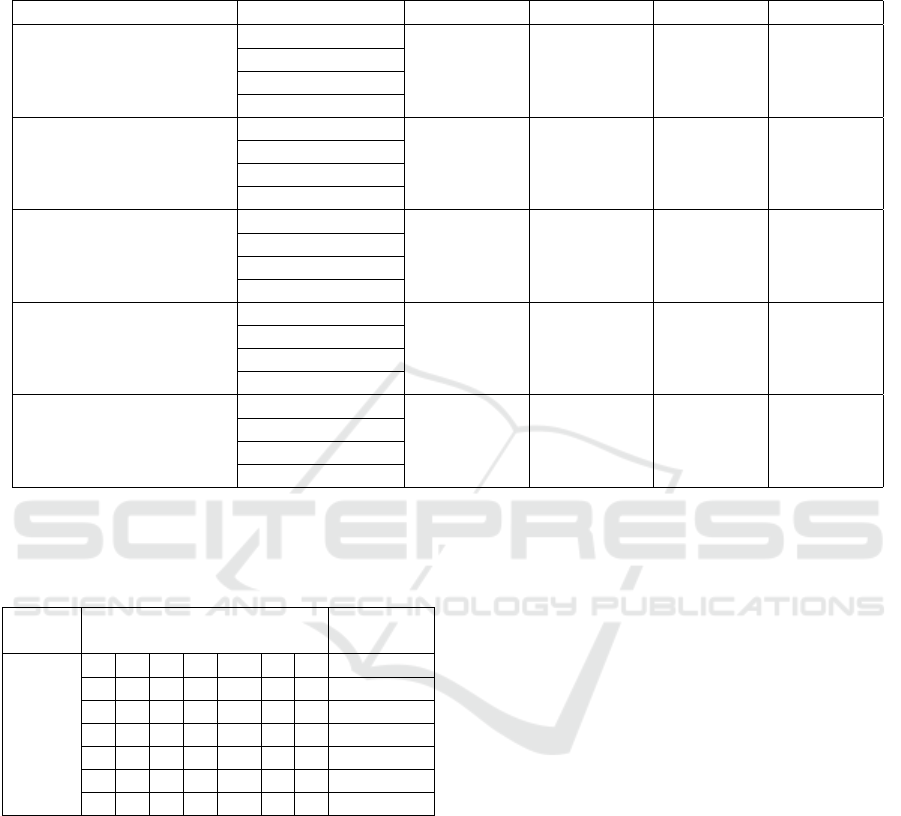
Table 2: Classiﬁcation performances of the proposed pipelines using different segmentation methods and GNN architectures.

Results are averages (with standard deviation) of performance measured over 3 shufﬂe splits validation. Layers and sizes of

each GNN architecture : {GNN1 : conv1 = 8, conv2 = 16, conv3 = 32, maxpool; GNN2 : conv1 = 8, conv2 = 16, conv3 = 32,

meanpool; GNN4 : conv1 = 16, conv2 = 32, conv3 = 64, maxpool; GNN4 : conv1 = 16, conv2 = 32, conv3 = 64, meanpool;}.

GNN architecture

Accuracy Recall Precision F1

GNN1 36.78 ± 4.34 0.34 ± 0.03 0.32 ± 0.03 0.33 ± 0.03

GNN2 35.63 ± 8.68 0.35 ± 0.05 0.32 ± 0.06 0.33 ± 0.05

GNN3 43.10 ± 8.62 0.37 ± 0.06 0.35 ± 0.02 0.37 ± 0.04

Histogram-based

n = 6

GNN4 41.95 ± 1.99 0.37 ± 0.03 0.38 ± 0.02 0.37 ± 0.01

GNN1 31.61 ± 4.34 0.33 ± 0.06 0.31 ± 0.03 0.32 ± 0.04

GNN2 33.33 ± 8.84 9.78 ± 16.32 0.30 ± 0.07 0.32 ± 0.08

GNN3 30.46 ± 2.63 0.30 ± 0.01 0.29 ± 0.03 0.29 ± 0.01

Histogram-based

n = 20

GNN4 37.92 ± 3.47 0.39 ± 0.04 0.35 ± 0.06 0.35 ± 0.04

GNN1 40.81 ± 7.78 0.42 ± 0.07 0.41 ± 0.08 0.42 ± 0.08

GNN2 37.36 ± 6.97 0.38 ± 0.07 0.35 ± 0.03 0.37 ± 0.03

GNN3 43.10 ± 6.90 0.47 ± 0.03 0.43 ± 0.04 0.42 ± 0.05

Histogram-based

n = 30

GNN4 40.81 ± 6.53 0.38 ± 0.08 0.39 ± 0.07 0.39 ± 0.08

GNN1 59.20 ± 8.15 0.60 ± 0.08 0.59 ± 0.10 0.59 ± 0.09

GNN2 48.28 ± 2.98 0.53 ± 0.05 0.53 ± 0.04 0.53 ± 0.04

GNN3 54.60 ± 7.18 0.57 ± 0.08 0.60 ± 0.11 0.58 ± 0.10

Split and merge

Split homogeneity = 10

Merge homogeneity = 40

GNN4 63.22 ± 5.27 0.62 ± 0.03 0.65 ± 0.07 0.62 ± 0.05

GNN1 49.05 ± 5.00 0.50 ± 0.04 0.51 ± 0.05 0.51 ± 0.04

GNN2 47.80 ± 4.36 0.49 ± 0.09 0.53 ± 0.11 0.51 ± 0.10

GNN3 47.80 ± 2.88 0.54 ± 0.06 0.53 ± 0.06 0.54 ± 0.06

Split and merge

Split homogeneity = 20

Merge homogeneity = 60

GNN4 41.51 ± 5.33 0.43 ± 0.08 0.48 ± 0.04 0.42 ± 0.07

Table 3: Confusion matrix of the ﬁrst “shufﬂe split” training

of the best conﬁguration which has a score of 63.79% of

accuracy.

Predicted classes

Prediction

rate

True

classes

6 1 2 1 0 0 0 6/10

1 3 0 0 0 0 0 3/4

0 0 3 2 1 0 0 3/6

0 0 1 4 1 0 0 4/6

0 0 2 2 12 3 0 12/19

0 0 1 1 2 4 0 4/8

0 0 0 0 0 0 5 5/5

distances and surface contact areas.

Future research will focus on exploring various con-

ﬁgurations and architectures to optimize our ap-

proach. More complex models, like NNConv or graph

attention layers, could be incorporated to better utilize

edge features. This approach enhances interpretabil-

ity, often lacking in CNN methods, and offers ﬂexibil-

ity in selecting scales or conducting multi-scale anal-

yses for deeper insights into data structures. GNNs

capture complex relationships, leading to more robust

models, making them superior for tasks requiring an

understanding of element relationships. Thus, we be-

lieve automatic segmentation for graph building and

GNN analysis is a promising solution.

ACKNOWLEDGEMENTS

We thank Scott Love for scientiﬁc and enthusiastic

discussions on brain MRI segmentations. We ac-

knowledge the ﬁnancial support the Institut National

de Recherche pour l’Agriculture, l’Alimentation et

l’Environnement D

epartement Physiologie Animale

(INRAE-PHASE) et Syst

emes d’

Elevage and the

egion Centre Val de Loire for the PhD grant for

Antoine Bourlier. The MR-images were acquired

in projects supported by INRAE - PHASE (Neu-

roimagery, PhenoMatHyp, Prebiostress) and by Val

de Loire regional council (Ovin2A, Convention 2013

00083140, coordinator R. Nowak, France; Neuro2Co,

Convention 2017 00117257, coordinator E. Chaillou,

France). This research was funded, in whole or in

part, by the French National Research Agency (ANR)

under the project ”ANR-23-SSAI-0008-01.” In line

with the objective of open-access publication, the au-

thor holder applies an open-access CC-BY license to

any accepted article (AAM) resulting from this sub-

mission.

Comparison Between CNN and GNN Pipelines for Analysing the Brain in Development

481

REFERENCES

Bullmore, E. T. and Bassett, D. S. (2011). Brain graphs:

Graphical models of the human brain connectome.

7:113–140.

Cai, H., Gao, Y., and Liu, M. (2023). Graph Trans-

former Geometric Learning of Brain Networks Us-

ing Multimodal MR Images for Brain Age Estimation.

42(2):456–466.

Cheng, J., Liu, Z., Guan, H., Wu, Z., Zhu, H., Jiang, J.,

Wen, W., Tao, D., and Liu, T. (2021). Brain Age

Estimation From MRI Using Cascade Networks With

Ranking Loss. 40(12):3400–3412.

Cole, J. H., Poudel, R. P. K., Tsagkrasoulis, D., Caan, M.

W. A., Steves, C., Spector, T. D., and Montana, G.

(2017). Predicting brain age with deep learning from

raw imaging data results in a reliable and heritable

biomarker. 163:115–124.

Coupeau, P., Fasquel, J. B., Mazerand, E., Menei, P.,

Montero-Menei, C. N., and Dinomais, M. (2022).

Patch-based 3D U-Net and transfer learning for

longitudinal piglet brain segmentation on MRI.

214:106563.

Cui, H., Dai, W., Zhu, Y., Li, X., He, L., and Yang, C.

(2021). BrainNNExplainer: An Interpretable Graph

Neural Network Framework for Brain Network based

Disease Analysis.

De Vico Fallani, F., Latora, V., and Chavez, M. (2017).

A Topological Criterion for Filtering Information in

Complex Brain Networks. 13(1):e1005305.

Ella, A., Delgadillo, J. A., Chemineau, P., and Keller, M.

(2017). Computation of a high-resolution MRI 3D

stereotaxic atlas of the sheep brain. 525(3):676–692.

Fedorov, A., Beichel, R., Kalpathy-Cramer, J., Finet, J.,

Fillion-Robin, J.-C., Pujol, S., Bauer, C., Jennings,

D., Fennessy, F., Sonka, M., Buatti, J., Aylward, S.,

Miller, J. V., Pieper, S., and Kikinis, R. (2012). 3D

Slicer as an Image Computing Platform for the Quan-

titative Imaging Network. 30(9):1323–1341.

Fil, J. E., Joung, S., Zimmerman, B. J., Sutton, B. P., and

Dilger, R. N. (2021). High-resolution magnetic res-

onance imaging-based atlases for the young and ado-

lescent domesticated pig (Sus scrofa). 354:109107.

Galisot, G., Ramel, J.-Y., Brouard, T., Chaillou, E., and Ser-

res, B. (2022). Visual and structural feature combi-

nation in an interactive machine learning system for

medical image segmentation. 8:100294.

Gonzalez, R. C. and Woods, R. E. (2017). Digital Image

Processing. Pearson, fourth edition, global edition

edition.

He, K., Zhang, X., Ren, S., and Sun, J. (2016). Deep Resid-

ual Learning for Image Recognition. In 2016 IEEE

Conference on Computer Vision and Pattern Recogni-

tion (CVPR), pages 770–778.

Jiang, H., Lu, N., Chen, K., Yao, L., Li, K., Zhang, J.,

and Guo, X. (2020). Predicting Brain Age of Healthy

Adults Based on Structural MRI Parcellation Using

Convolutional Neural Networks. 10.

Kaur, P. and Gaba, G. S. (2021). Computational Neuro-

science Models and Tools: A Review. In Bhoi, A. K.,

Mallick, P. K., Liu, C.-M., and Balas, V. E., editors,

Bio-Inspired Neurocomputing, Studies in Computa-

tional Intelligence, pages 403–417. Springer.

Krizhevsky, A., Sutskever, I., and Hinton, G. E. (2012). Im-

ageNet Classiﬁcation with Deep Convolutional Neu-

ral Networks. In Advances in Neural Information Pro-

cessing Systems, volume 25. Curran Associates, Inc.

Lam, P., Zhu, A. H., Gari, I. B., Jahanshad, N., and Thomp-

son, P. M. (2020). 3D Grid-Attention Networks for

Interpretable Age and Alzheimer’s Disease Prediction

from Structural MRI.

Li, G., Wang, L., Yap, P.-T., Wang, F., Wu, Z., Meng, Y.,

Dong, P., Kim, J., Shi, F., Rekik, I., Lin, W., and

Shen, D. (2019). Computational neuroanatomy of

baby brains: A review. 185:906–925.

Li, X., Zhou, Y., Dvornek, N., Zhang, M., Gao, S., Zhuang,

J., Scheinost, D., Staib, L. H., Ventola, P., and Duncan,

J. S. (2021). BrainGNN: Interpretable Brain Graph

Neural Network for fMRI Analysis. 74:102233.

Lim, H., Joo, Y., Ha, E., Song, Y., Yoon, S., and Shin, T.

(2024). Brain Age Prediction Using Multi-Hop Graph

Attention Combined with Convolutional Neural Net-

work. 11(3):265.

Nitzsche, B., Frey, S., Collins, L. D., Seeger, J., Lobsien,

D., Dreyer, A., Kirsten, H., Stoffel, M. H., Fonov,

V. S., and Boltze, J. (2015). A stereotaxic, population-

averaged T1w ovine brain atlas including cerebral

morphology and tissue volumes. 9.

Park, H.-J. and Friston, K. (2013). Structural and Func-

tional Brain Networks: From Connections to Cogni-

tion. 342(6158):1238411.

Poriya, V. (2023). Brain Tumor Classiﬁcation And Segmen-

tation Using Machine Learning For Magnetic Reso-

nance Images.

Ravinder, M., Saluja, G., Allabun, S., Alqahtani, M. S., Ab-

bas, M., Othman, M., and Souﬁene, B. O. (2023). En-

hanced brain tumor classiﬁcation using graph convo-

lutional neural network architecture. 13(1):14938.

Schmid, S. (2023). Image Intensity Normalization in Med-

ical Imaging.

Sporns, O. (2007). Brain connectivity. 2(10):4695.

Sporns, O. (2018). Graph theory methods: Applications in

brain networks. 20(2):111–121.

Srinivasan, S., Francis, D., Mathivanan, S. K., Rajadurai,

H., Shivahare, B. D., and Shah, M. A. (2024). A hy-

brid deep CNN model for brain tumor image multi-

classiﬁcation. 24(1):21.

Van Essen, D. C. and Drury, H. A. (1997). Structural and

Functional Analyses of Human Cerebral Cortex Using

a Surface-Based Atlas. 17(18):7079–7102.

Yang, G., Zhou, S., Bozek, J., Dong, H.-M., Han, M., Zuo,

X.-N., Liu, H., and Gao, J.-H. (2020). Sample sizes

and population differences in brain template construc-

tion. 206:116318.

VISAPP 2025 - 20th International Conference on Computer Vision Theory and Applications

482