Improving Locally Differentially Private Graph Statistics Through
Sparseness-Preserving Noise-Graph Addition
Sudipta Paul
1 a
, Juli
´
an Salas
2 b
and Vicenc¸ Torra
1 c
1
Department of Computing Science, Ume
˚
a Universitet, Ume
˚
a, Sweden
2
Department of Information and Communications Engineering,
Universitat Aut
`
onoma de Barcelona, Bellaterra, Spain
Keywords:
Privacy in Large Network, Differential Privacy, Edge Local Differential Privacy.
Abstract:
Differential privacy allows to publish graph statistics in a way that protects individual privacy while still
allowing meaningful insights to be derived from the data. The centralized privacy model of differential privacy
assumes that there is a trusted data curator, while the local model does not require such a trusted authority.
Local differential privacy is commonly achieved through randomized response (RR) mechanisms. This does
not preserve the sparseness of the graphs. As most of the real-world graphs are sparse and have several nodes,
this is a drawback of RR-based mechanisms, in terms of computational efficiency and accuracy. We thus,
propose a comparative analysis through experimental analysis and discussion, to compute statistics with local
differential privacy, where, it is shown that preserving the sparseness of the original graphs is the key factor
to gain that balance between utility and privacy. We perform several experiments to test the utility of the
protected graphs in terms of several sub-graph counting i.e. triangle, and star counting and other statistics. We
show that the sparseness preserving algorithm gives comparable or better results in comparison to the other
state of the art methods and improves computational efficiency.
1 INTRODUCTION
Real-world networks are made of sensitive entities
and relations which carry meaningful patterns, for
example: interbank payment networks, internet and
World Wide Web networks, protein-protein interac-
tion networks, and airline networks.
Graph Statistics (Brinkmeier and Schank, 2005),
such as average degree, subgraph counts (triangles,
stars or cliques), community structure and central-
ity measures, are analysed to describe essential prop-
erties of the network. For example, the subgraph
counts can be used to measure the clustering coeffi-
cient, which measures the probability that two friends
of an individual will also be friends with one another.
When the information is sensitive, analysing
graph data while still preserving the privacy of the
individuals is very important. Differentially private
graph analysis is one of the main approaches to
analysing graphs in a privacy-preserving way. The
a
https://orcid.org/0000-0001-6561-997X
b
https://orcid.org/0000-0003-1787-0654
c
https://orcid.org/0000-0002-0368-8037
vast majority of algorithms for differentially private
graph analysis fall into the centralized (or global)
paradigm, in which all the information is held by a
single trusted data curator who publishes a masked
copy of the information, or a statistic of the data.
For security and privacy reasons, a single curator
may be inadequate, as the centralized data repository
can be compromised and data leaked. Local Differ-
ential Privacy (LDP) is an alternative that can be used
for untrusted servers, where data is anonymized lo-
cally and only anonymized data will be shared with
a central server. Two main LDP definitions exist for
graphs, one focuses on node differential privacy and
the other on edge differential privacy.
In this paper, we focus on local edge differential
privacy for graphs. We will see how step by step, the
usage of different algorithms promises to mitigate dif-
ferent practical drawbacks of edge local differential
privacy and how sparseness preservation becomes the
key to gaining a better utility and privacy balance in
the shortest run time.
The contributions of our work are the following:
1. Experimentally we show that sparseness preserva-
tion in large networks improves the privacy-utility
526
Paul, S., Salas, J. and Torra, V.
Improving Locally Differentially Private Graph Statistics Through Sparseness-Preserving Noise-Graph Addition.
DOI: 10.5220/0013174400003899
Paper published under CC license (CC BY-NC-ND 4.0)
In Proceedings of the 11th International Conference on Information Systems Security and Privacy (ICISSP 2025) - Volume 2, pages 526-533
ISBN: 978-989-758-735-1; ISSN: 2184-4356
Proceedings Copyright © 2025 by SCITEPRESS – Science and Technology Publications, Lda.

balance,
2. The sparseness-preserving algorithm works faster,
and
3. The sparseness-preserving algorithm shows com-
parable or better results than the state of the art
algorithms.
The later part of the paper is arranged in the fol-
lowing way: we give preliminaries to what Graph DP,
LDP and the previous approaches towards counting
statistics look like with and without DP in Sec. 2.
This is followed by a detailed discussion of the algo-
rithms in Sec. 3. After that, we explain the exper-
iments and the comparative analysis for all of these
algorithms from different angles in Sec. 4. We finish
with a conclusion and future scope of work in Sec. 5.
2 BACKGROUND KNOWLEDGE
In this section, we will explore the related background
knowledge to further understand the algorithms using
differential privacy for graphs.
Differential privacy (DP) (Dwork, 2006) is one
of the well established privacy models. There are two
categories: centralized differential privacy and local
differential privacy (LDP). The centralized model as-
sumes centralized data collection. So, all users’ orig-
inal personal data is gathered by a “trusted” data col-
lector, who then obscures a query (such as a counting
query or a histogram query) on the set of personal
data. In contrast, in LDP, the data collector is not
trusted. The users protect locally their own data and
only submit the protected data to the collector. Two
types of LDP mechanisms have been proposed for
graphs: edge LDP and node LDP (Jian et al., 2021).
In edge LDP, protection is such that a release should
not disclose the presence or absence of an edge. As
opposed to this, in node LDP, protection is such that
a release should not disclose the presence or absence
of a node. We will be using edge LDP in this work.
The formal definition of DP is based on the concept of
neighbouring databases. In the context of edge DP for
graphs, two neighbouring graphs G, G
′
∈ G, where G
denotes the set of graphs, are two graphs that differ in
only one edge. Then, the definition is based on ε, a
privacy budget. Maximum privacy is for ε = 0, and
the larger the ε, the lower the privacy guarantees.
To understand Edge Local Differential Privacy,
we need to understand ε-local differential privacy
first. Now, LDP is used in the local model to safe-
guard each user’s personal information. On the other
hand, every edge in a graph is linked to two users.
Therefore, we should take our desired level of pro-
tection into account while defining edge DP in the
local model. We took the definition of ε-local dif-
ferential privacy straight from the article (Cormode
et al., 2018). A randomized algorithm π, satisfies ε-
local differential privacy if for all inputs x,x
′
and all
outputs y ∈ Range(π):
Pr(π(x) = y) ≤ e
ε
Pr(π(x
′
) = y) (1)
we say that π is ε-locally differentially private (ε-
LDP).
Edge Local Differential Privacy (eLDP) can be
defined as follows from the definition of (Imola et al.,
2021) and (Qin et al., 2017):
Let ε ∈ R≥ 0. For any i ∈ [n], let A
i
be a random-
ized algorithm of user u
i
with domain {0,1}
n
. Then
for any two neighbour lists a
i
,a
′
i
∈ {0,1}
n
which dif-
fer by one bit and any S ⊆ Range(A
i
), A
i
gives ε−edge
LDP, if it satisfies,
Pr[A
i
(a
i
) ∈ S] ≤ e
ε
Pr[A
i
(a
′
i
) ∈ S] (2)
Eq. 2 protects a single bit in the neighbour list with the
privacy budget ε where the assumption is taken that
two users are not sharing knowledge. But this is not
the case in graph data. To acknowledge this (Imola
et al., 2021) used the Relationship DP concept.
We need some additional concepts. They are
Global Sensitivity, Randomised Response and Privacy
amplification by Shuffling
The Global Sensitivity of any function f : D → R
is given by
GS
f
= max
D,D
′
∈D:D∼D
′
|f(D) − f(D
′
)| (3)
Where, D ∼ D
′
means that D and D
′
are neighbours,
that is, they differ by one edge in edge centralised DP
and one bit in edge LDP.
Warner’s Randomised Response (Warner, 1965)
applied to a neighbor list can be defined like
this: let x
i
∈ {0,1}
n
be a neighbour list and y =
(y
1
,y
2
,..., y
n
) ∈ {0,1}
n
is the output of the Ran-
domised Response algorithm for x
i
. Here, each bit
of x
i
has been flipped with the probability p =
1
e
ε
+1
,
i.e. for each j ∈ [n], y
j
̸= x
i j
with probability p and
with probability 1 − p it remains the same y
j
= x
i j
.
According to Eq. 1 the definition of ε-local differen-
tial privacy, when x
i
and x
′
i
differ only by a bit then
Pr(π(x
i
) ∈ S) and Pr(π(x
′
i
) ∈ S) differ in proportion
by e
ε
. In this way, the RR algorithm yields the ε-local
differential privacy.
Privacy amplification by Shuffling is based on an
Encode-Shuffle-Analyze Architecture in which each
user sends her encrypted and obfuscated data to an
intermediate server which randomly shuffles the ob-
fuscated data of all users, and sends it to the data col-
lector to decrypt them. The shuffling amplifies DP
guarantees by improving the utility for the same ε.
Improving Locally Differentially Private Graph Statistics Through Sparseness-Preserving Noise-Graph Addition
527

This model was first proposed by (Bittau et al.,
2017) and is called “Prochlo”. The results here show
that when inputs are shuffled before local randomiz-
ers are applied, privacy is “amplified” and remains in-
tact even in cases when local randomizers are selected
both adaptively and sequentially. But this model is
primarily for tabular data and in their work (Imola
et al., 2022b) adopted it to be workable for the graph
data as well.
3 RELATED WORK
In this section, we present graphs statistics, non-
private algorithm to count them and their eLDP ver-
sions.
Average Degree is an important characteristic of
large graphs. The average degree provides a sum-
mary of the degree distribution. Estimating the de-
gree distribution of a big graph using a small, ran-
dom sample is the aim of a substantial body of liter-
ature on graph sampling (Dasgupta et al., 2014). In
their work, Kasiviswanathan et al. (Kasiviswanathan
et al., 2013) using a simple projection function which
can be written as f
T
: G → G
θ
, provides a way that
releases privacy-preserved degree distribution of the
graph G, where the function f
T
discards all nodes
whose degrees are higher than a threshold θ. Blocki et
al. (Blocki et al., 2022) proposed a differentially pri-
vate sublinear-time (1 + ρ) approximation algorithm
for the computing of average degree for every ρ > 0,
where the runtime is the same as the non-private state
of the art version. They used coupled global sensitiv-
ity to formalize the unifying framework for the pri-
vacy analysis. Goldreich et al.’s (Goldreich and Ron,
2008) results indicate that for the private approxima-
tion of the average degree, the problem-specific or-
acle with neighbour queries helps. Their algorithm
obtains an approximation of (1 + ε) where, ε > 0 to
the average degree of a simple graph G = (V,E) in
time O(
p
|V |) where it has a polynomial dependence
of
1
ε
.
Triangle counting is one of the basic subgraph
counting algorithms. It is also a required step for com-
puting the average clustering coefficient. The non-
private approaches consist of Brute Force approach:
it has complexity O(n
3
), checks every possible triplet
of vertices to see if they form a triangle; Edge It-
eration Algorithm (Becchetti et al., 2010): O(n
3/2
),
iterates over edges and use adjacency lists to check
for triangles; Matrix Multiplication-Based Algorithm
(Avron, 2010): O(n
2.376
), e.g. Strassen’s Algorithm
uses fast Matrix multiplication; Adjacency Matrix Al-
gorithm (Chu and Cheng, 2011): O(n
3
), it computes
A
3
the cube of the adjacency matrix and uses the trace
to count the triangles; Color Coding Algorithm (Bres-
san et al., 2021): O(n
3
), a randomized algorithm that
colors vertices; Spectral Methods (Tsourakakis et al.,
2011): they use eigenvalues and eigenvectors of the
adjacency matrix to count the triangles; MapReduce-
based Algorithms (Park and Chung, 2013); Graph
Sparsification (Tsourakakis, 2008): O(n
3/2
), it reduce
the number of edges while preserving triangle count
properties, then use the algorithm to count the tri-
angles; and Approximation algorithm (Arifuzzaman
et al., 2019), (Tsourakakis et al., 2009): it provides
an approximate count of triangles using sampling or
other heuristic methods.
Imola et al. (Imola et al., 2021) proposed two
eLDP triangle counting algorithms. Let G be the orig-
inal graph and the user v
i
is not aware if it is a part of
the triangle formed by (v
i
,v
j
,v
k
) as v
i
can not see any
the v
j
v
k
edge. In the 1
st
algorithm (LocalRR
∆
) the
user v
i
applies RR to its neighbour list a
i
i.e. the RR
is being applied to the lower triangular part of the ad-
jacency matrix A. Then the data collector constructs
a noisy graph G
′
from the noisy lower triangular ma-
trix A
′
after the RR is applied to A and estimates the
number of triangles using the “edge iteration based
approach”. In the 2
nd
algorithm (Local2Rounds
∆
),
they added empirical estimation to unbias the triangle
counting, by dividing the ε budget into three parts (as
a subgraph with three nodes can be divided into four
types, i.e. 3-nodes with 3 edges, 2-edges, 1-edge and
no edge). Another aspect of these algorithms is that
they use adaptive clipping to privately estimate the
highest degree d
max
to significantly reduce the global
sensitivity which will be later used to estimate the
local adjacency graph. But these suffer from huge
per-user download costs i.e. 400 GB or more when
n ≥ 900000 because the data collector has to down-
load the whole noisy graph. To remedy that Imola
et al. proposed three algorithms under edge-LDP in
(Imola et al., 2022a). The strategies that they opted
to remedy the situation are: 1) sampling edges and 2)
selecting edges per user download. They used sam-
pling edges for each user v
i
after the RR was done.
Therefore the main research question they actually
tried to answer is: “Which noisy edges should each
user v
i
download at the second round?” The three
solutions are: 1) ARRFull
∆
: to download all noisy
edges between others; 2) ARROneNS
∆
: to make two
noisy triangles less correlated to each other by select-
ing one noisy edge that is connected between (v
j
,v
k
);
and 3) ARRTwoNS
∆
: to make two noisy triangles
less correlated to each other by selecting two noisy
edges that are connected to v
i
from (v
j
,v
k
). How-
ever, in all approaches, there is an extremely large es-
ICISSP 2025 - 11th International Conference on Information Systems Security and Privacy
528

timation error assuming multi-round interaction, ef-
fort plus synchronization between the user and data
collector. To mitigate that Imola et al. (Imola et al.,
2022b) proposed a three-phased algorithm depending
upon the shuffling model (Cheu et al., 2019). Those
are the Wedge Shuffle Algorithm (W S), Wedge Shuf-
fling with Local Edges (W SLE) and unbiased esti-
mation of the number of the triangles (W Shu f f le
∆
).
Here “Wedge” means 2-hop paths between 2 definite
pair of users namely v
i
and v
j
. In the W S algorithm
the other user v
k
given the two users v
i
and v
j
calcu-
lates a wedge-indicator w
i−k− j
= a
k,i
a
k, j
, which as-
signs the value 1 if a wedge v
i
− v
k
− v
j
exists or 0.
Then v
k
masks the w
i−k− j
using the ε
L−RR
and then
sends the wedge to the shuffler. The shuffler then ran-
domly shuffles the noisy wedges with a random per-
mutation π and then the shuffler sends the shuffled
wedges to the data collector. To further reduce the
variance they proposed WShu f f le
∗
∆
which ignores the
sparse user-pairs.
Star counting refers to small subgraphs where a
central node is connected to several peripheral nodes.
Star subgraphs are important for analyzing network
structures (Aliakbarpour et al., 2018), (Gonen et al.,
2011), as they often represent central actors (hubs)
connected to many others. In social networks, a star
structure might represent an influencer or a popular
figure, while in large technical networks, it could rep-
resent critical nodes in communication systems. The
non-private approach includes: Brute Force Algo-
rithm (O(nd
2
), for each vertex, count the number
of pairs of its neighbours to identify star structures),
Degree-Based Counting (Kolountzakis et al., 2012)
(Ahmed et al., 2015) (O(n + m), iterate through each
vertex v and use its degree d
v
to count the number of
stars it forms

d
v
2

=
d
v
(d
v
−1)
2
), Matrix Multiplication
based algorithm (O(n
2
), use the adjacency matrix to
count 2-paths (paths of length 2) through each ver-
tex. The number of such 2-paths for a vertex v can be
derived from the square of the adjacency matrix) and
Dynamic Programming on Trees (Chakraborty et al.,
2018) (O(n) for tree Structures. If the graph is a tree
or forest, dynamic programming techniques can be
used to count stars efficiently by processing subtrees).
The edge LDP approach (LocalLap
k∗
) (Imola
et al., 2021) to star counting typically involves a ran-
domized response mechanism. Each participant (or
node) perturbs their connections with a certain prob-
ability before sending this information to the central
server. The server can then use aggregate statistics
to estimate the true structure of the network, includ-
ing the presence of star structures, without directly
accessing any individual’s true connections.
In the above discussion, one thing is clear, every
algorithm has ignored preserving the sparseness in the
adjacency matrix and later in the result part in Section
4 we will see that the sparseness preservation is the
key to have the balance between utility and privacy.
Noise graph addition was defined in (Torra and
Salas, 2019) and it was later shown that eLDP and
sparseness guarantees can be obtained from such
mechanism by adjusting the probabilities of random-
ization, as in (Salas et al., 2023). We take the defini-
tion of Noise-Graph Mechanism straight from (Salas
et al., 2023) as follows:
For any graph G with n nodes, and two probabil-
ities p
0
and p
1
, we define the following noise-graph
mechanism:
A
p
0
,p
1
(G) = G ⊕ G
0
⊕ G
1
,
such that:
E(G
0
) = E(G
′
) \ E(G) and E(G
1
) = E(G
′′
) ∩ E(G)
where G
′
and G
′′
are drawn respectively from:
G(n,1 − p
0
) and G(n,1 − p
1
) following the Gilbert
Model. It was shown that probabilities commonly
used for the RR mechanisms yield denser graphs
with an expected density of: (1 −
2
e
ε
+1
)
q
(
n
2
)
+
2
e
ε
+1
,
where q denotes the number of edges in the original
graph (Salas et al., 2023). However, using the dif-
ferent parametrizations from (Salas et al., 2022), an
appropriate combination of probabilities can be ob-
tained to preserve the sparseness of the original graph.
We will test the utility of such sparseness preserv-
ing randomizations in triangle and star counting with
eLDP.
4 RESULTS AND ANALYSIS
In this section, we explain our extensive experimen-
tal results and their analysis with the help of several
graph statistics counts.
4.1 Experiment Description
We have considered the three datasets described in Ta-
ble 1. They have different number of vertices ranging
30724 to 896308, and they have different sparseness.
The system specification for the experiment is -
UBUNTU 20.04.2 LTS, 64-bit Kernel Linux 5.8.0-
44-generic x86 64 FOCAL FOSSA 1.20.4 OS with
32.6 GiB of memory and Intel(R) Xeon(R) W-1250P
CPU @ 4.10GHz. The R-studio with R-4.4.1 (2024-
06-14) – ”Race for Your Life” has been used, with
a steady internet connection of 881.83 Mbit/s down-
load speed and a 898.74 Mbit/s upload speed. We also
Improving Locally Differentially Private Graph Statistics Through Sparseness-Preserving Noise-Graph Addition
529

Table 1: Descriptions of the datasets used in the experiment.
Name No. of Edges No. of Vertices Average Degree Sparseness
IMDB 57064358 896308 63.7 3.55E-6
Orkut 117185083 3072441 38.1 6.2E-6
Gplus 1048572 70974 14.7 0.00041
have a NVIDIA GeForce RTX 3060 GPU component
with the driver Version: 560.35.03 and CUDA Ver-
sion: 12.6.
We compared LocalRR
∆
(Imola et al.,
2021), ARRTwoNS
∆
(Imola et al., 2022a),
W Shu f f le
∗
∆
(Imola et al., 2022b), Noisy-Graph (Salas
et al., 2022) and Sparseness-Preserving (Salas et al.,
2023) algorithms. We did the experiments in two
parts. For the first part, the experiment can be
divided into three steps: 1) Pre-Processing: We
randomly choose 10000 vertices from all the datasets,
2) Building the graph: We extract the edge set for
each vertex from the edge set of the network datasets
and build the graph for each randomly chosen dataset
from the previous step. For IMDB dataset we
retrieved a graph containing 896308 nodes, where
each node represents one actor. In this graph, an edge
connecting two actors/nodes indicates that they have
been in the same film. For Gplus dataset an edge con-
necting two nodes/users is defined that either follows
each other or one is followed by the other, and lastly,
3) We then run all 5 methods 100 times for each of
the vertex sets and epsilon values. To implement the
Noise-graph and Sparseness preservation methods
there is an extra step that we took before the third step
and that is epsilon calculation. Also, in the Figures
1, 2 and 3, we took the results for the 10000 users
and plotted the average with the standard deviation
with changing epsilons. For the second part of the
experiment, we took the whole dataset in the case
of IMDB and GPlus. But for Orkut, we could only
work with 660692 nodes and 1048574 edges from the
original dataset because of our limited computational
resources. We repeat the same steps as the first part 5
times except for the random sampling here.
4.2 Results and Discussion
Table 1 provides average degree of the three data
sets. So, these are the desired values for privacy-
preserving solutions for the average degree. It can
be seen that in terms of sparseness, IMDB is sparser
than others. Then, Orkut and finally Gplus which
is the most dense. From the plotted results in Fig-
ures 1, 2, and 3 (A), we can observe that, as expected,
the larger the epsilon, the Sparseness preserving al-
gorithms work better. That is, the less protection, the
larger the utility. The figures show the variance of
the experiment for each epsilon value. Among the
algorithms, Sparseness preserving and WShuffle pro-
vide better results. A rough ranking of the methods
is: Sparseness preserving > WShuffle > ARRTwoNS
> LocalRR > Noise-graph. From the definition of
average degree, it is known that it is proportional to
the number of edges. In case of both the Sparseness
preserving and WShuffle algorithms, the graph density
is always in the neighbourhood of the true value. In
the first case, the samples are constant and the added
noise has changed in all the iterations. If we see the
steps of the WShuffle algorithm, very little noise is
added to the wedges through shuffling, which in a
way preserves the true density value. At the same
time through m-random perturbation and threshold
random sparsification techniques the Sparseness pre-
serving algorithm also does the same but in a better
and faster way.
We have two sets of experimental results for the
triangle counting statistics. For the first part of exper-
iment, from the plotted result in Figure 1, 2, 3(C), the
Sparseness preserving and WShuffle algorithms again
work the best in terms of utility for every dataset.
But with bigger epsilon values (> 0.75), Sparseness
preserving, ARRTwoNS and WShuffle algorithms have
given better or comparable results in terms of utility
and the LocalRR algorithm has given comparable re-
sult in case of the IMDB dataset with the others for
ε > 0.8. One explanation for this is the presence
of sparseness preservation. But when the number of
nodes or vertices increases the algorithms LocalRR,
ArrTwoNS, WShuffle becomes slower. It is evident
from the Table 2 that the Sparseness preserving al-
gorithm is faster. The Sparseness preserving algo-
rithm gives better results in terms of utility too, for
the whole graph, which we can see in Figure 4. In
these three figures, in terms of absolute error, we ob-
serve that for LocalRR, Noisy-graph and ArrTwoNS
the triangle counts are from 6 to 8 orders of mag-
nitude higher than the original counts, while WShuf-
fle and Sparseness-preserving algorithms are compet-
itive and quite accurate in the counts. Still, for smaller
epsilon values sparseness-preserving algorithm ob-
tains the best results.
The clustering coefficient (Zhang et al., 2008)
measures the tendency of nodes to form triangles. The
clustering coefficient for a node v is defined as:
C(v) = 3 × triangles/all triplets (4)
ICISSP 2025 - 11th International Conference on Information Systems Security and Privacy
530

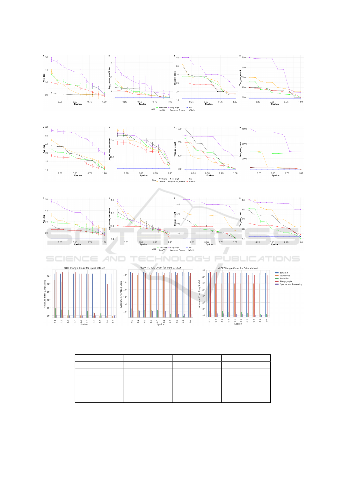
Figure 1: Result for IMDB data with different 10000 random sampling everytime.
Figure 2: Result for Orkut data with different 10000 random sampling everytime.
Figure 3: Result for Gplus data with different 10000 random sampling everytime.
Figure 4: Absolute Error for the eLDP Triangle Counts for Gplus, IMDB and Orkut dataset.
Table 2: Average wall clock time for each of the algorithm’s run time for the whole dataset (except Orkut) in seconds for
Triangle Counting.
Algorithm IMDB Orkut Gplus
LocalRR 120.5 190.5 135.5
ARRTwoNS 75.1 82.3 60.1
WShuffle 73.1 81.1 60.1
Noise-graph 10.2 12.7 9.4
Sparseness-
Preserving
4.8 6.1 4.4
Improving Locally Differentially Private Graph Statistics Through Sparseness-Preserving Noise-Graph Addition
531

We can see that it is directly proportional to the trian-
gle counts. Therefore, the trend of results is similar
to that of the triangle counting. In case of both the
Sparseness preserving and WShuffle algorithms, the
graph density is being tuned so that it is always in
the neighbourhood of the true value. If we see the
WShuffle algorithm, very little noise is added to the
wedge through shuffling, which in a way preserves
the true density value. At the same time through
m-random perturbation and threshold random spar-
sification techniques the Sparseness preserving algo-
rithm also does the same but in a better way. There-
fore the number of triangles is not changing drasti-
cally while working with these two algorithms. From
the plotted result in Figure 1, 2, 3(B), we can see
that as the epsilon increases (> 0.75) the Sparseness
preserving and WShuffle algorithms work the best in
terms of utility in general.
From the plotted result in Figure 1, 2, 3(D) it
is evident that WShuffle and Sparseness-preserving
algorithms both perform similarly in terms of
utility-privacy balance for all the datasets and the
performance is far better than others in case of
the 2-star Count. Though the standard deviation
has increased in the case of GPlus dataset when
the ε > 0.75, but for every dataset WShuffle and
Sparseness-preserving algorithms perform better
than others. So if we put a ranking for IMDB
data: Noisy − graph < LocalRR < ARRTwoNS <
Sparseness − Preserving ∼ W Shu f f le. The
same in the case of Orkut dataset would be
Noisy − graph < ARRTwoNS < LocalRR <
Sparseness − Preserving ∼ W Shu f f le. For GPlus
dataset this ranking would be Noisy − graph <
LocalRR < Sparseness − Preserving ∼ W Shu f f le <
ARRTwoNS.
In conclusion for a bigger dataset with more nodes
and edges Sparseness-Preserving algorithm seems to
work better in terms of utility and timing than the oth-
ers. Also, due to the Random Perturbation and Ran-
dom Sparsification technique while forcing a sparse-
ness threshold helps it to perform better or compara-
ble to the WShuffle algorithm.
5 CONCLUSION AND FUTURE
SCOPE
We compared different private triangle and star count-
ing algorithms for graphs. We can see from the ex-
perimental results that preserving the sparseness of
the graphs is the key to a faster and more precise
way to privately calculate the graph metrics. We saw
how from the mere randomised response to counting
4-cycle and double clipping to wedge shuffling im-
proves the speed and the “privacy-utility” trade-off
but overlooks the sparseness of the graph. Lastly, we
see that by preserving the sparseness in a lot sim-
pler way all these can be achieved in lesser time.
Therefore, this comparative study in both theoreti-
cal and experimental domain establishes that sparse-
ness preserving is a better option both computation-
ally and communication overhead wise for counting
basic graph statistics. As a future work, it remains to
calculate a broader range of statistics on the protected
graphs with the Sparseness-Preserving algorithm.
ACKNOWLEDGMENTS
This work was partially supported by the Wallen-
berg AI, Autonomous Systems and Software Pro-
gram (WASP) funded by the Knut and Alice Wal-
lenberg Foundation. Support by the Swedish Re-
search Council under the project Privacy for com-
plex data (VR 2022-04645) is also acknowledged.
Project DANGER C062/23 within the Plan de Recu-
peraci
´
on, Transformaci
´
on y Resiliencia funded with
Next Generation EU funds, Spanish Ministry under
Grant PID2021-125962OB-C33 SECURING/NET,
and Catalan AGAUR under Grant SGR2021-00643
are also acknowledged.
REFERENCES
Ahmed, N. K., Neville, J., Rossi, R. A., and Duffield, N.
(2015). Efficient graphlet counting for large networks.
In 2015 IEEE international conference on data min-
ing, pages 1–10. IEEE.
Aliakbarpour, M., Biswas, A. S., Gouleakis, T., Pee-
bles, J., Rubinfeld, R., and Yodpinyanee, A. (2018).
Sublinear-time algorithms for counting star subgraphs
via edge sampling. Algorithmica, 80:668–697.
Arifuzzaman, S., Khan, M., and Marathe, M. (2019). Fast
parallel algorithms for counting and listing triangles
in big graphs. ACM Transactions on Knowledge Dis-
covery from Data (TKDD), 14(1):1–34.
Avron, H. (2010). Counting triangles in large graphs using
randomized matrix trace estimation. In Workshop on
Large-scale Data Mining: Theory and Applications,
volume 10, page 9.
Becchetti, L., Boldi, P., Castillo, C., and Gionis, A.
(2010). Efficient algorithms for large-scale local trian-
gle counting. ACM Transactions on Knowledge Dis-
covery from Data (TKDD), 4(3):1–28.
Bittau, A., Erlingsson,
´
U., Maniatis, P., Mironov, I., Raghu-
nathan, A., Lie, D., Rudominer, M., Kode, U., Tinnes,
J., and Seefeld, B. (2017). Prochlo: Strong privacy for
ICISSP 2025 - 11th International Conference on Information Systems Security and Privacy
532

analytics in the crowd. In Proceedings of the 26th sym-
posium on operating systems principles, pages 441–
459.
Blocki, J., Grigorescu, E., and Mukherjee, T. (2022). Pri-
vately estimating graph parameters in sublinear time.
arXiv preprint arXiv:2202.05776.
Bressan, M., Leucci, S., and Panconesi, A. (2021). Faster
motif counting via succinct color coding and adaptive
sampling. ACM Transactions on Knowledge Discov-
ery from Data (TKDD), 15(6):1–27.
Brinkmeier, M. and Schank, T. (2005). Network statis-
tics. In Network analysis: methodological founda-
tions, pages 293–317. Springer.
Chakraborty, M., Milani, A., and Mosteiro, M. A. (2018).
A faster exact-counting protocol for anonymous dy-
namic networks. Algorithmica, 80:3023–3049.
Cheu, A., Smith, A., Ullman, J., Zeber, D., and Zhilyaev,
M. (2019). Distributed differential privacy via shuf-
fling. In Advances in Cryptology–EUROCRYPT 2019:
38th Annual International Conference on the The-
ory and Applications of Cryptographic Techniques,
Darmstadt, Germany, May 19–23, 2019, Proceedings,
Part I 38, pages 375–403. Springer.
Chu, S. and Cheng, J. (2011). Triangle listing in mas-
sive networks and its applications. In Proceedings
of the 17th ACM SIGKDD international conference
on Knowledge discovery and data mining, pages 672–
680.
Cormode, G., Jha, S., Kulkarni, T., Li, N., Srivastava, D.,
and Wang, T. (2018). Privacy at scale: Local differen-
tial privacy in practice. In Proceedings of the 2018 In-
ternational Conference on Management of Data, SIG-
MOD ’18, page 1655–1658, New York, NY, USA. As-
sociation for Computing Machinery.
Dasgupta, A., Kumar, R., and Sarlos, T. (2014). On esti-
mating the average degree. In Proceedings of the 23rd
international conference on World wide web, pages
795–806.
Dwork, C. (2006). Differential privacy. In International col-
loquium on automata, languages, and programming,
pages 1–12. Springer.
Goldreich, O. and Ron, D. (2008). Approximating aver-
age parameters of graphs. Random Structures & Al-
gorithms, 32(4):473–493.
Gonen, M., Ron, D., and Shavitt, Y. (2011). Counting stars
and other small subgraphs in sublinear-time. SIAM
Journal on Discrete Mathematics, 25(3):1365–1411.
Imola, J., Murakami, T., and Chaudhuri, K. (2021). Locally
differentially private analysis of graph statistics. In
30th USENIX security symposium (USENIX Security
21), pages 983–1000.
Imola, J., Murakami, T., and Chaudhuri, K. (2022a).
{Communication-Efficient} triangle counting under
local differential privacy. In 31st USENIX security
symposium (USENIX Security 22), pages 537–554.
Imola, J., Murakami, T., and Chaudhuri, K. (2022b). Dif-
ferentially private triangle and 4-cycle counting in
the shuffle model. In Proceedings of the 2022 ACM
SIGSAC Conference on Computer and Communica-
tions Security, pages 1505–1519.
Jian, X., Wang, Y., and Chen, L. (2021). Publishing graphs
under node differential privacy. IEEE Transactions on
Knowledge and Data Engineering, 35(4):4164–4177.
Kasiviswanathan, S. P., Nissim, K., Raskhodnikova, S., and
Smith, A. (2013). Analyzing graphs with node differ-
ential privacy. In Theory of Cryptography: 10th The-
ory of Cryptography Conference, TCC 2013, Tokyo,
Japan, March 3-6, 2013. Proceedings, pages 457–
476. Springer.
Kolountzakis, M. N., Miller, G. L., Peng, R., and
Tsourakakis, C. E. (2012). Efficient triangle counting
in large graphs via degree-based vertex partitioning.
Internet Mathematics, 8(1-2):161–185.
Park, H.-M. and Chung, C.-W. (2013). An efficient mapre-
duce algorithm for counting triangles in a very large
graph. In Proceedings of the 22nd ACM interna-
tional conference on Information & Knowledge Man-
agement, pages 539–548.
Qin, Z., Yu, T., Yang, Y., Khalil, I., Xiao, X., and Ren,
K. (2017). Generating synthetic decentralized social
graphs with local differential privacy. In Proceedings
of the 2017 ACM SIGSAC conference on computer
and communications security, pages 425–438.
Salas, J., Gonz
´
alez-Zelaya, V., Torra, V., and Meg
´
ıas,
D. (2023). Differentially private graph publishing
through noise-graph addition. In International Con-
ference on Modeling Decisions for Artificial Intelli-
gence, pages 253–264. Springer.
Salas, J., Torra, V., and Meg
´
ıas, D. (2022). Towards measur-
ing fairness for local differential privacy. In Interna-
tional Workshop on Data Privacy Management, pages
19–34. Springer.
Torra, V. and Salas, J. (2019). Graph perturbation as
noise graph addition: a new perspective for graph
anonymization. In Data Privacy Management, Cryp-
tocurrencies and Blockchain Technology: ESORICS
2019 International Workshops, DPM 2019 and CBT
2019, Luxembourg, September 26–27, 2019, Proceed-
ings 14, pages 121–137. Springer.
Tsourakakis, C. E. (2008). Fast counting of triangles in
large real networks without counting: Algorithms and
laws. In 2008 Eighth IEEE International Conference
on Data Mining, pages 608–617. IEEE.
Tsourakakis, C. E., Drineas, P., Michelakis, E., Koutis, I.,
and Faloutsos, C. (2011). Spectral counting of tri-
angles via element-wise sparsification and triangle-
based link recommendation. Social Network Analysis
and Mining, 1:75–81.
Tsourakakis, C. E., Kolountzakis, M. N., and Miller,
G. L. (2009). Approximate triangle counting. arXiv
preprint arXiv:0904.3761.
Warner, S. L. (1965). Randomized response: A survey tech-
nique for eliminating evasive answer bias. Journal of
the American statistical association, 60(309):63–69.
Zhang, P., Wang, J., Li, X., Li, M., Di, Z., and Fan, Y.
(2008). Clustering coefficient and community struc-
ture of bipartite networks. Physica A: Statistical Me-
chanics and its Applications, 387(27):6869–6875.
Improving Locally Differentially Private Graph Statistics Through Sparseness-Preserving Noise-Graph Addition
533