Models and Algorithms for the Optimization of Multi-Period Fiber

Wholesale Investments Strategies

Youssouf Hadhbi

, Aur

elien Bechler

and Matthieu Chardy

Orange Innovation, Ch

atillon, France

{youssouf.hadhbi, aurelien.bechler, matthieu.chardy}@orange.com

Keywords:

Fiber Wholesale Markets, Investment Strategies, Multi-Period Portfolio Optimization, Mixed-Integer Linear

Program, Valid Inequalities, Branch-and-Cut.

Abstract:

This paper focuses on optimizing multi-period investment strategies for Fiber deployment. The main ob-

jective is to provide guidelines to improve the cost-effectiveness of Fiber investment strategies employed by

telecommunication operators. To achieve this objective, an optimization framework is developed, providing

a systematic approach to multi-period investment planning for Fiber deployment. It combines mathematical

modeling and data analysis. For this, we introduce two mixed-integer linear programs to formulate the prob-

lem, taking into account demands, budget constraints and market conditions. Additionally, we propose several

valid inequalities for the associated polytopes to enhance the linear relaxation and achieve tighter bounds.

Relying on this modeling framework, we devise an exact optimization approach based on a Branch-and-Cut

algorithm to solve the problem. Furthermore, we present a computational study that considers various in-

stances and scenarios to assess the performance of the proposed models and algorithms.

1 INTRODUCTION

The transformation of copper access networks into

Fiber optic networks is a key challenge for telecom-

munication operators such as Orange, in terms of eco-

nomic viability, competition, and inclusion, with the

aim of providing sustainable and quality telecommu-

nication services to everyone.

1.1 Telecom Context and Motivations

In Europe, ﬁxed broadband subscriptions are pro-

jected to increase by 25 million, rising from 260 mil-

lion in 2021 to 285 million by 2026 (Dgtlinfra, 2021).

Fiber is anticipated to become the dominant trans-

mission technology, with its subscriptions growing

from 30% in 2021 to over 50% by 2026 (Dgtlinfra,

2021). This transition underscores the signiﬁcance of

various network architecture options utilizing optical

ﬁber, collectively referred to as Fiber To The x. Here,

”x” represents the Fiber termination point, which can

be at home (FTTH), curb (FTTC), building (FTTB),

antenna (FTTA), or premises (FTTP). Fiber To The x

https://orcid.org/0000-0001-8032-087X

https://orcid.org/0009-0003-0119-891X

https://orcid.org/0009-0003-9137-4605

is crucial for next-generation access, signiﬁcantly en-

hancing broadband speed and quality of service (QoS)

(Dgtlinfra, 2021).

In France, the ”Plan France Tr

es Haut D

ebit”

(PFTHD) is designed to achieve high-speed broad-

band coverage across the entire national territory, tar-

geting all homes, businesses, and public administra-

tions by 2030. The initiative is projected to cost a total

of 21 billion euros, with public investment expected

to account for approximately 13 billion euros to 14

billion euros. In particular, the cost of deploying the

FTTH technology across the entire territory has been

estimated at several dozen billion euros by the French

Senate (Angilella et al., 2016). Consequently, opera-

tors do not deploy their own FTTH networks through-

out the whole territory; especially, in speciﬁc geo-

graphical areas, deployments are entrusted to third-

party operators.

The key question for a commercial operator like

Orange becomes deﬁning an effective long-term strat-

egy for aquiring optical ﬁbers in the areas deployed by

third-party operators, covering the needs of its cus-

tomers while minimizing purchasing costs. The asso-

ciated ﬁnancial stakes amount to several hundred mil-

lion euros per year, making the optimization of such

strategy essential.

This study primarily focuses on optimizing the

Hadhbi, Y., Bechler, A. and Chardy, M.

Models and Algorithms for the Optimization of Multi-Period Fiber Wholesale Investments Strategies.

DOI: 10.5220/0013182900003893

Paper published under CC license (CC BY-NC-ND 4.0)

In Proceedings of the 14th International Conference on Operations Research and Enterprise Systems (ICORES 2025), pages 133-145

ISBN: 978-989-758-732-0; ISSN: 2184-4372

133

Fiber infrastructure business decision, especially in

these geographical areas where third-party operators

are in charge of the Fiber deployment. This involves

strategically choosing the level of investment in Fiber

optic infrastructure to meet the customers’demand for

high-speed and connectivity from which is increas-

ing over time. Due to limited investment capacity, it

is necessary to consider the multi-year nature of Fiber

wholesale investments. This also holds signiﬁcant im-

portance because investment decisions in the telecom-

munication networks often have long-term implica-

tions. By developing effective investment strategies,

we aim to assist telecommunication operators in max-

imizing the impact and beneﬁts of their investment ef-

forts. Moreover, the study enables telco to plan their

investments strategically, considering factors such as

future demand forecasts, budget constraints, so as to

remain competitive in the dynamic Fiber wholesale

market. This paper explores the strategic planning

of Fiber optic deployment across multiple zones that

are currently undeployed. Each zone has speciﬁc at-

tributes, including the number of connectable clients

and demand for connections over consecutive time

periods. The operator can choose between two in-

vestment strategies: renting or co-investment of Fiber

lines, with the requirement that the total deployed

lines meet the demand. Zones are classiﬁed based on

investment feasibility, and the decision-making pro-

cess is inﬂuenced by investment percentages and cu-

mulative investment rates, which must adhere to con-

tractual limits. Investments incur capital and opera-

tional costs, with a budget constraint on capital ex-

penditures. The study focuses on optimizing invest-

ment strategies to effectively meet client demands

while managing costs. Moreover, this study exam-

ines several key performance indicators (KPIs) essen-

tial for evaluating the success of investment decisions

in Fiber optic infrastructure. The metrics analyzed in-

clude Return on Investment (ROI), which measures

the cost-effectiveness of investments by comparing

generated beneﬁts to initial costs; Capital Expendi-

ture (CAPEX) costs, which encompass funds allo-

cated for acquiring or upgrading infrastructure; and

Operational Expenditure (OPEX) costs, reﬂecting on-

going expenses related to maintenance and energy

consumption. Additionally, the analysis embeds Fiber

renting costs, which are critical when existing Fiber

lines do not meet demand, and Fiber migration costs,

incurred when transitioning from rented to co-owned

Fiber lines. By assessing these KPIs, the study aims

to provide a comprehensive framework for informed

investment decision-making in the Fiber optic sector,

providing decision-makers with insights to improve

the economic viability of Fiber optic deployments.

1.2 Related Works

Regarding the literature, extensive research has been

conducted on the optimization of investment strate-

gies for various energy-related challenges. These in-

clude:

• Renewable Energy Systems: studies such as those

by (Wang et al., 2020),(Farah and Andresen,

2024) and (Faria et al., 2023) have explored in-

novative investment strategies to enhance the ef-

ﬁciency and sustainability of renewable energy

sources.

• Power Grid Management: research by (Gao et al.,

2022), (Gao et al., 2023) and (Zhang et al., 2019)

has focused on optimizing investments in power

grid infrastructure, aiming to improve reliability

and reduce operational costs.

• Energy Efﬁciency: the work of (He et al., 2019)

has highlighted strategies to optimize investments

in energy-efﬁcient technologies, contributing to

overall energy savings.

• Smart Grids: studies by (Giannelos et al., 2023),

(Tuballa and Abundo, 2016) and (Zafar et al.,

2018) have examined investment optimization in

smart grid technologies, emphasizing the integra-

tion of advanced communication and control sys-

tems.

Conversely, some research has investigated invest-

ments in battery storage within telecommunications

networks, particularly under energy market incen-

tives, as seen in the works of (Kerdphol et al., 2016)

and (Silva et al., 2024). However, the speciﬁc area

of optimizing investment strategies for Fiber deploy-

ment, particularly in FTTH networks, remains under-

explored in the current state of the art. Most research

on Fiber optic network design has mainly focused on

network planning themselves and not the investment

optimization. (Gr

otschel et al., 2014) studied the cost-

effective deployment of optical access networks, fo-

cusing on different variants such as ﬁber to the home,

ﬁber to the building, ﬁber to the curb, and ﬁber to the

neighborhood. Other studies, such as (Chardy et al.,

2012), (Hervet et al., 2012), (Angilella et al., 2016)

and (Angilella et al., 2018), have addressed this topic,

focusing on the ﬁber to the home. Additionally, some

research has proposed optimization approaches for

mobile networks, as demonstrated by (Cambier et al.,

2021) and (Zappal

a et al., 2022). This presents an

opportunity for further investigation into investment

strategies that could enhance Fiber deployment efﬁ-

ciency and effectiveness in telecommunications.

ICORES 2025 - 14th International Conference on Operations Research and Enterprise Systems

134

1.3 Contributions

In the work, we aim to provide an optimization

framework for network operators to optimize their

investment strategies speciﬁcally for Fiber deploy-

ment. This can be considered as the ﬁrst devel-

oped framework in the literature to address this novel

economic problem encountered in Fiber deployment.

Our framework aims to provide an optimization ap-

proach to manage the investment strategies and min-

imizing costs in Fiber deployment scenarios. To

achieve this, we believe that an optimization approach

based on mathematical models and exact optimiza-

tion algorithms can effectively solve this problem,

even when dealing with large instances. For this,

we provide an efﬁcient solution to the challenges

raised by the problem using mixed integer linear pro-

gramming formulations (MILP), and a polyhedral ap-

proach based on a Branch-and-Cut (B&C) algorithm.

1.4 Organization of the Paper

The rest of this paper is organized as follows. In Sec-

tion 2, we provide a detailed step-by-step description

of the problem, which we refer to as the Multi-Period

Fiber Wholesale Investment Strategies Optimization

(MP-FWIS-O) problem. We consider the MP-FWIS-

O as a combinatorial optimization problem and pro-

vide its intuitive formulation as a Mixed Integer Lin-

ear Program. Section 3 is dedicated to the Complexity

analysis of the problem. In Section 4, we present sev-

eral mathematical properties leading us to reformulate

the problem, as well as a range of valid inequalities

for both formulation. A Branch-and-Cut is presented

in Section 5. We then present an extensive compu-

tational study in Section 6 using different classes of

instances and scenarios. Finally, we summarize our

results and future outlook in Section 7.

2 PROBLEM DESCRIPTION AND

FORMULATION

We consider a geographical area (typically a country)

composed of a set of zones Z, on which the deploy-

ment of the Fiber access network is granted to ded-

icated Infrastructure Operators o

, z ∈ Z. These de-

ployments spread over time and we thus consider a

discrete time horizon T = {1, .., n}, over which we

assume the future deployments to be known with cer-

tainty, denoting D

z,t

the number of Fiber lines de-

ployed on zone z ∈ Z up to period t ∈ T ∪ {0} (ie. the

connectable customers), t = 0 denoting the last period

in the past that comes before the ﬁrst period in T .

We focus on a speciﬁc commercial operator of the

geographical area (typically a domestic operator such

as Orange) and denote by d

z,t

,t ∈ T ∪{0} the temporal

evolution of its number of retail Fiber customers on

zone z ∈ Z.

Considering any zone z ∈ Z and in order to be able

to satisfy its retail customers, this commercial opera-

tor has to purchase physical Fiber lines by the Infras-

tructure Operator of the zone o

mixing two comple-

mentary purchasing strategies: co-investing in the de-

ployments and renting lines. As for the co-investment

strategy, we assume that the commercial operator can

invest at particular periods T

⊂ T when investment

committees hold, and only on a speciﬁc set of invest-

ment slices denoted by I and numbered from 0 to 20

(i.e., I = {0, 1, 2, ..., 19, 20}). We model the opera-

tor’s co-investment decisions by binary variables c

upg

z,t,i

equal to 1 if the operator decides to make a new co-

investment on slice i ∈ I for zone z ∈ Z at period t ∈ T

(0 otherwise), leading to the acquisition of a number

of new Fiber lines equal to a percentage Q

of the

deployed Fiber lines for the rest of the time-horizon

(note that we assume Q

= 0% so as to model a ”no-

investment” slice, indexed by 0). Speciﬁcally, the set

)

i∈I

consists of slice percentages ranging from 0%

to 100% in increments of 5% (for example Q

is equal

to 35%). At any time-period t ∈ T , based on its se-

quence of previous co-investments, the operator thus

owns a percentage of the deployed Fiber lines D

z,t

for

each zone z ∈ Z, denoted by positive continuous vari-

able q

z,t

≥ 0 (note that this variable q

z,t

will, in prac-

tice, take value within the set (Q

)

i∈I

). Introducing

constant parameter q

z,0

the value of the initial cumu-

lative investment rate at period t = 0, the dynamics

can be described by the following equations:

z,t

= q

z,t−1

∑

i∈I

· c

upg

z,t,i

, ∀z ∈ Z, ∀t ∈ T, (1)

while ensuring that at most one slice is invested on

each zone at any time-period

∑

i∈I

upg

z,t,i

= 1, ∀z ∈ Z, ∀t ∈ T, (2)

and that no investments are made outside committees’

time-periods:

∑

i∈I\{0}

upg

z,t,i

= 0, ∀t ∈ T \T

. (3)

Note that for regulatory motivations related to fairness

(among domestic operators notably), a maximum in-

vestment rate, denoted by Q

max

and assumed to be

greater than q

z,0

, is set on each zone z ∈ Z, such that:

z,t

≤ Q

max

, ∀t ∈ T. (4)

Models and Algorithms for the Optimization of Multi-Period Fiber Wholesale Investments Strategies

135

From this dynamics, we can derive the number of co-

ﬁnanced Fiber lines for each zone z ∈ Z and at each

period t ∈ T , denoted by

z,t

= D

z,t

· q

z,t

, ∀z ∈ Z, ∀t ∈ T . (5)

In this context, considering any zone z ∈ Z and period

t ∈ T , the whole number of retail Fiber customers of

the operator must be covered either by using a part of

its co-ﬁnanced Fiber lines, denoted by u

inv

z,t

, or rented

lines u

rent

z,t

inv

z,t

+ u

rent

z,t

= d

z,t

, ∀z ∈ Z, ∀t ∈ T, (6)

knowing that the number of co-ﬁnanced Fiber lines

used to serve customers cannot exceed the number of

co-ﬁnanced Fiber lines owned by the operator:

inv

z,t

≤

z,t

, ∀z ∈ Z, ∀t ∈ T . (7)

Mixed co-investments and renting strategies induce

several types of costs. First, co-investments made in

zone z ∈ Z at period t ∈ T lead to one-shot capital

expenditures (CAPEX) which are proportional to the

number of Fiber lines ”acquired” at this period and

for this zone, denoted by positive continuous variable

capex

z,t

. Precisely, newly acquired Fiber lines can re-

sult from two phenomena identiﬁed in the following

CAPEX cost formulation:

capex

z,t

= CAPEX

z,t

∑

i∈I

· D

z,t

· c

upg

z,t,i

+ Q



z,t

− D

z,t−1



· c

tot

z,t−1,i

, ∀z ∈ Z, ∀t ∈ T , (8)

where CAPEX

z,t

stands for the unitary cost of acquir-

ing a new Fiber line at period t ∈ T for zone z ∈ Z,

and



z,t

−D

z,t−1



= max



0;D

z,t

−D

z,t−1



. For any

zone z ∈ Z we set constants c

tot

z,0,i

, ∀i ∈ I to 0 except

for the unique slice i ∈ I such that q

z,0

= Q

, which is

set to 1.

On the other hand, for any zone z ∈ Z at any period

t ∈ T , the use of any co-ﬁnanced Fiber line incurs an

operational cost (OPEX) depending on the total co-

investment slice, denoted by SUB

z,t,i

where i ∈ I rep-

resents the index of the total co-investment slice at

period t. To derive such type of cost, we ﬁrst need

to identify the slice associated to a given total invest-

ment rate. Introducing binary variables c

tot

z,t,i

equal to 1

if the cumulative investment rate is equal to Q

, i ∈ I,

we identify the unique total co-investment slice for

each zone z ∈ Z and period t ∈ T as follows:

z,t

∑

i∈I

· c

tot

z,t,i

, ∀z ∈ Z, ∀t ∈ T , (9)

∑

i∈I

tot

z,t,i

= 1, ∀z ∈ Z, ∀t ∈ T . (10)

Then the OPEX cost, noted opex

z,t

, can be expressed

as follows:

opex

z,t

∑

i∈I

SUB

z,t,i

· c

tot

z,t,i

· u

inv

z,t

, ∀z ∈ Z, ∀t ∈ T. (11)

The non-linearity of equations (11) is evident. To deal

with this, we propose a new variable f

inv

z,t,i

∈ Z

which

denotes the number of co-owned invested and used

Fiber lines when we have cumulatively the ith slice of

investment in zone. Using this, we consider the in-

equalities (11-1)-(11-4) used to linearize and replace

the quadratic equation (11). For each z ∈ Z and t ∈ T

opex

z,t

∑

i∈I

SUB

z,t,i

· f

inv

z,t,i

. (11-1)

For each z ∈ Z, i ∈ I and t ∈ T , we ensure that

inv

z,t,i

≤ u

inv

z,t

, (11-2)

inv

z,t,i

≤ Q

· D

z,t

· c

tot

z,t,i

, (11-3)

inv

z,t

− Q

· D

z,t

· (1 − c

tot

z,t,i

) ≤ f

inv

z,t,i

. (11-4)

Second, the renting cost of each zone z ∈ Z and period

t ∈ T is proportional to the number of rented lines. Let

RENT

z,t

denote the unitary renting cost. The cumu-

lative renting cost is expressed through the decision

variables rent

z,t

, deﬁned as follows:

rent

z,t

= RENT

z,t

· u

rent

z,t

, ∀z ∈ Z, ∀t ∈ T . (12)

Finally, at any period t ∈ T , a unitary migration cost

MIG

z,t

is applied to any Fiber line rented at period

t − 1 and then served by a co-ﬁnanced Fiber line at

period t, in the speciﬁc case of t being the ﬁrst co-

investment period. Introducing the incremental de-

mand ∆d

z,t

= d

z,t

− d

z,t−1

for each zone z ∈ Z and pe-

riod t ∈ T and denoting respectively by u

inv

z,0

and u

rec

z,0

the initial number of co-invested and rented ﬁbers for

each zone z ∈ Z at period t = 0, the number of mi-

grated ﬁbers can be computed by distinguishing two

cases:

• when the number of Fiber customers decreases

from period t −1 to t, the number of migrated cus-

tomers at t is precisely the number of customers

served by co-invested ﬁbers at t, ie. u

inv

z,t

− u

inv

z,t−1

• when the number of Fiber customers increases

from period t − 1 to t, the number of migrated

customers at t corresponds to the decrease in the

number of retail customers served with rented

lines u

rent

z,t−1

− u

rent

z,t

This is summarized in the following equalities:

mig

z,t

= ⊮

{∆d

z,t

≤0}

inv

z,t

− u

inv

z,t−1

) (13)

+ ⊮

{∆d

z,t

>0}

rent

z,t−1

− u

rent

z,t

), ∀z ∈ Z, ∀t ∈ T .

We notice that the ﬁrst period of co-investment

is, if existing, the only period t ∈ T such that

ICORES 2025 - 14th International Conference on Operations Research and Enterprise Systems

136

∑

i∈I\{0}

tot

z,t,i

− c

tot

z,t−1,i

= 1. Then the migration cost,

denoted by decision variables mig

z,t

for each zone

z ∈ Z and period t ∈ T , can be bounded as follows:

mig

z,t

≥ MIG

z,t

· u

mig

z,t

− d

z,t

∑

i∈I\{0}

tot

z,t,i

− c

tot

z,t−1,i

(14)

relying on the objective function to ensure its equality

to 0 when needed.

Finally, we assume that the co-investments strate-

gies are restrained by CAPEX budgets attributed to

each investment committee period t ∈ T

, denoted by

Budget

. Denoting P

the set of periods between t and

the next committee, we thus consider the following

constraints for each committee period t ∈ T

∑

z∈Z

∑

′

∈P

capex

z,t

′

≤ Budget

. (15)

Note that the basis of this formulation enables to

consider different objective functions that are mean-

ingful for a network operator, such as minimizing

• the total weighted sum of renting, opex and mi-

gration costs

min

∑

z∈Z

∑

t∈T

α · rent

z,t

+ β · opex

z,t

+ λ · mig

z,t

(16)

• the total weighted sum of renting and migrated

Fiber lines

min

∑

z∈Z

∑

t∈T

α · u

rent

z,t

+ β · u

mig

z,t

, (17)

• the total number of not used co-ﬁnancer Fiber

lines

min

∑

z∈Z

∑

t∈T

z,t

− u

inv

z,t

, (18)

where α, β, λ ∈ R.

Moreover, these objective functions can be used as

metrics to evaluate the solution of the problem, con-

sidering other KPIs as mentioned in the introduction.

For the sake of clarity, we consider a small-size

example with one single zone (denoted by z) and a

4-periods time horizon T = {1, 2, 3, 4} with a unique

investment committee positionned at the second pe-

riod (T

= {2}) where we choose to invest on the

ﬁrst slice (with Q

= 5%). Table 1 provides a fea-

sible solution so as to illustrate both the decision no-

tation and the cost computation mechanisms. Note

that, under the assumption that unitary renting costs

are strictly greater than unitary operationnal costs

(SUB

z,t,i

< RENT

z,t

, ∀t ∈ T, ∀i ∈ I), this solution is not

optimal as using u

inv

z,3

= 45 co-ﬁnanced lines at

period 3 (and thus renting u

rent

z,3

= 17 Fiber lines) in-

stead of using u

inv

z,3

= 39 co-ﬁnanced lines (and thus

Table 1: Illustration of notation and feasible solution to the

MP-FWIS-O problem.

T 0 1 2 3 4

z,t

0 500 800 900 1000

z,t

0 20 37 61 49

upg

z,t,i

- 0 c

upg

z,2,1

= 1 0 0

tot

z,t,i

tot

z,0,0

= 1 c

tot

z,2,0

= 1 c

tot

z,2,1

= 1 c

tot

z,3,1

= 1 c

tot

z,4,1

= 1

z,t

0% 0% 5% 5% 5%

z,t

- 0 40 45 50

capex

z,t

- 0 40 CAPEX

z,2

5 CAPEX

z,3

5 CAPEX

z,4

inv

z,t

0 0 37 39 49

opex

z,t

- 0 37 SUB

z,2,1

39 SUB

z,3,1

49 SUB

z,4,1

rent

z,t

0 20 0 22 0

rent

z,t

- 20 RENT

z,1

0 22 RENT

z,3

mig

z,t

- 0 20 0 10

mig

z,t

- 0 20 MIG

z,2

0 0

renting u

rent

z,3

= 22 Fiber lines) would lead to a lower

objectif cost.

In this study, our focus is primarily on the objec-

tive function (16) with α, β and λ equal to 1, as these

3 types of costs are operationnal costs.

In additon, we will denote

P (Z, T, T

, I, Q, D, d, Budget) the polytope asso-

ciated to (in)equations (1) to (15).

In the following section, we will study the com-

plexity of the MP-FWIS-O problem.

3 PROBLEM COMPLEXITY

From a complexity point of view, the MP-FWIS-O

problem becomes polynomial when the budget con-

straints are relaxed and the objective is to minimize

certain costs such as the total renting cost, the total

migration cost and the total OPEX cost. In such sce-

narios, the problem can be efﬁciently and optimally

solved in polynomial time (Cook, 1971). However,

when facing strict budget constraints, the problem be-

comes more complex, and ﬁnding an optimal solution

within polynomial time becomes challenging. In gen-

eral, we believe that this problem is NP-hard, meaning

that it is computationally difﬁcult to solve optimally

in polynomial time (Cook, 1971). In particular, the

knapsack problem can be viewed as a speciﬁc case of

the problem when limited to a single investment com-

mittee period. The knapsack problem is a well-known

combinatorial optimization problem, where the goal

is to select a subset of items with maximum value

while respecting a capacity constraint. The knapsack

problem has shown to be NP-hard. It can be seen as a

mathematical representation of the budget-constraint.

The knapsack’s capacity corresponds to the budget

constraint, and the items represent various investment

options or slices that can be chosen within that con-

straint. The objective is to ﬁnd the combination of

Models and Algorithms for the Optimization of Multi-Period Fiber Wholesale Investments Strategies

137

items that maximizes the overall value or utility, sim-

ilar to how one would aim to optimize multiple costs

within a limited budget.

4 KEY ENHANCEMENTS

In this section, we investigate properties of the MP-

FWIS-O problem and derive potential enhancements

for the basic formulation provided in Section 2, lead-

ing us to propose a reformulation for the problem. In

addition we provide valid inequalities for both formu-

lations.

4.1 Properties on Optimal Solutions

First, we introduce some properties related to the op-

timality of solutions.

Proposition 1. For each zone z ∈ Z, period t ∈ T and

slice i ∈ I , let us deﬁne

z,t,i

⌊

· D

z,t

⌋

Then, equation

z,t

∑

i∈I

· D

z,t,i

· c

tot

z,t,i

, ∀z ∈ Z, ∀t ∈ T (5.1)

is valid for the polytope

P (Z, T, T

, I, Q, D, d, Budget).

Note that integrating equations (5.1) instead of (5) in

the formulation ensures the integrality of variables

Proposition 2. Assuming a hierarchy in costs pa-

rameters (typically we have SUB

z,t,i

< RENT

z,t

∀z ∈

Z ∀t ∈ T, ∀i ∈ I), the integrality of variables u

inv

, u

rent

and u

mig

is ensured in any optimal solution when c

upg

and c

tot

are integers.

Based on this property, we will replace constraints (5)

by (5.1) and relax the integrality constraints on the

variables

d, u

inv

, u

rent

and u

mig

in the reformulation

given in Section 4.3.

Proposition 3. For any zone z ∈ Z, let us deﬁne

= min{Q

, i ∈ I : max

t∈T

z,t

≤ Q

Then, assuming strictly positive unitary CAPEX costs

(CAPEX

z,t

> 0, ∀z ∈ Z, ∀t ∈ T ), there exists an opti-

mal solution which satisﬁes:

z,t

≤ max(

z,0

), ∀z ∈ Z, ∀t ∈ T.

In the rest of the article, we deﬁne ¯q

min(Q

max

;max(

z,0

)).

4.2 Compactness

For the reformulation proposed in Section 4.3, we aim

at decreasing the number of variables and constraints

compared to the one provided in Section 2. For this,

we consider variables c

upg

z,t,i

, c

tot

z,t,i

, q

z,t

, u

mig

z,t

and mig

z,t

only for periods in T

. Therefore, we introduce func-

tion the following fonction C which provides the pe-

riod corresponding to latest committee anterior to t

within the time horizon (and 0 if no commitee oc-

cured):

C :



T −→ T

∪ {0}

t 7−→



0 if T

∩ {1, ...,t} =

max[T

∩ {1, ...,t}] otherwise

On the other hand, several former constraints need

consequently to be modiﬁed accordingly. The follow-

ing propositions present reformulated constraints that

will be utilized in the reformulation, while remaining

valid for P (Z, T, T

, I, Q, D, d, Budget).

Proposition 4. Consider a zone z ∈ Z and a period

t ∈ T

. Then, the following inequalities

z,t

= q

z,C(t−1)

∑

i∈I

· c

upg

z,t,i

(

z,t

≤ ¯q

(

capex

z,t

= CAPEX

z,t

∑

i∈I

· D

z,t

· c

upg

z,t,i



z,t

− D

z,t−1



· c

tot

z,C(t−1),i

(8.1)

mig

z,t

= ⊮

{∆d

z,t

≤0}

inv

z,t

− u

inv

z,t−1

)

+⊮

{∆d

z,t

>0}

rent

z,t−1

− u

rent

z,t

) (

13)

mig

z,t

≥ MIG

z,t

· u

mig

z,t

− d

z,t

∑

i∈I\{0}

tot

z,t,i

− c

tot

z,C(t−1),i

(

14)

are valid for the polytope

P (Z, T, T

, I, Q, D, d, Budget).

Proposition 5. Consider a zone z ∈ Z and a period

t ∈ T \ T

. Then, the following inequalities

z,t

∑

i∈I

· D

z,t,i

· c

tot

z,C(t),i

, (

capex

z,t

= CAPEX

z,t

∑

i∈I



z,t

− D

z,t−1



· c

tot

z,C(t−1),i

(8.2)

opex

z,t

∑

i∈I

SUB

z,t,i

· c

tot

z,C(t),i

· u

inv

z,t

, (

11)

are valid for the polytope

P (Z, T, T

, I, Q, D, d, Budget).

ICORES 2025 - 14th International Conference on Operations Research and Enterprise Systems

138

Remark1: Inequalities (4) have been revised at the

light of Proposition 3, incorporating the changes

made by considering only periods T

Remark2: Equation (8) needs to be modiﬁed by con-

sidering it only for t ∈ T

and introducing additional

equations for the rest of periods in T \ T

as follows:

capex

z,t

= CAPEX

z,t

∑

i∈I



z,t

− D

z,t−1



· c

tot

z,t−1,i

(8.2)

4.3 Reformulation

Based on the previous results, we reformulate the MP-

FWIS-O problem as follows:

min

∑

z∈Z

∑

t∈T

rent

z,t

+ opex

z,t

∑

t∈T

mig

z,t

, (

16)

subject to

z,t

= q

z,C(t−1)

∑

i∈I

· c

upg

z,t,i

, ∀z ∈ Z, ∀t ∈ T

, (

∑

i∈I

upg

z,t,i

= 1, ∀z ∈ Z, ∀t ∈ T

, (

z,t

≤ ¯q

, ∀z ∈ Z, ∀t ∈ T

, (

z,t

∑

i∈I

· D

z,t,i

· c

tot

z,C(t),i

, ∀z ∈ Z ∀t ∈ T, (

inv

z,t

+ u

rent

z,t

= d

z,t

, ∀z ∈ Z, ∀t ∈ T, (6)

inv

z,t

≤

z,t

, ∀z ∈ Z, ∀t ∈ T, (7)

capex

z,t

= CAPEX

z,t

∑

i∈I

· D

z,t

· c

upg

z,t,i



z,t

− D

z,t−1



· c

tot

z,C(t−1),i

, ∀z ∈ Z, ∀t ∈ T

, (8.1)

capex

z,t

= CAPEX

z,t

∑

i∈I



z,t

− D

z,t−1



· c

tot

z,C(t−1),i

∀z ∈ Z, ∀t ∈ T \ T

, (8.2)

z,t

∑

i∈I

· c

tot

z,t,i

, ∀z ∈ Z, ∀t ∈ T

, (

∑

i∈I

tot

z,t,i

= 1, ∀z ∈ Z, ∀t ∈ T

, (

10)

opex

z,t

∑

i∈I

SUB

z,t,i

· c

tot

z,C(t),i

· u

inv

z,t

, ∀z ∈ Z, ∀t ∈ T, (

11)

rent

z,t

= RENT

z,t

· u

rent

z,t

, ∀z ∈ Z, ∀t ∈ T, (12)

mig

z,t

= ⊮

{∆d

z,t

≤0}

inv

z,t

− u

inv

z,t−1

) + ⊮

{∆d

z,t

>0}

rent

z,t−1

− u

rent

z,t

∀z ∈ Z, ∀t ∈ T

, (

13)

mig

z,t

≥ MIG

z,t

· u

mig

z,t

− d

z,t

∑

i∈I\{0}

tot

z,t,i

− c

tot

z,C(t−1),i

∀z ∈ Z, ∀t ∈ T

, (

14)

∑

z∈Z

∑

′

∈P

capex

z,t

′

≤ Budget

, ∀z ∈ Z, ∀t ∈ T

, (15)

upg

z,t,i

, c

tot

z,t,i

∈ {0, 1}, ∀z ∈ Z, ∀t ∈ T

, ∀i ∈ I,

capex

z,t

, rent

z,t

, opex

z,t

, u

rent

z,t

, u

inv

z,t

≥ 0, ∀z ∈ Z, ∀t ∈ T,

z,t

, u

mig

z,t

, mig

z,t

≥ 0, ∀z ∈ Z, ∀t ∈ T

Note that equations (

11) need to be linearized, as

previously mentioned.

The formulations presented in Section 2

and in this section will be respectively re-

ferred to as MILPI and MIPLII. Moreover, let

P (Z, T, T

, I, Q, D, d, Budget) denote the polytope

associated with Formulation MILPII, representing the

convex hull of solutions obtained by satisfying all the

constraints previously presented in our reformulation,

while imposing integrality constraints for certain

variables.

4.4 Valid Inequalities

In what follows, we will introduce several valid in-

equalities to enhance the linear relaxation of our

formulations. These inequalities are intended to

strengthen the bounds of the linear relaxation. By

incorporating these additional constraints, we can

achieve more accurate and efﬁcient solutions.

Based on inequalities (4), we introduce the fol-

lowing inequality ensuring the non selection of cer-

tain slices i in I having a Q

bigger than the maximum

investement rate ¯q

Proposition 6. Consider a zone z ∈ Z. Then, the fol-

lowing inequality

∑

t∈T

∑

i∈I

> ¯q

tot

z,t,i

∑

i∈I

z,0

> ¯q

upg

z,t,i

= 0, (19)

is valid for the polytope

P (Z, T, T

, I, Q, D, d, Budget).

Proposition 7. Consider a zone z ∈ Z and a period

t ∈ T. Let i be a slice in I. Then, the following in-

equalities

tot

z,t,i

≤

∑

′

∈I

′

≥Q

tot

z,t+1,i

′

, (20)

tot

z,t,i

∑

′

∈I

′

tot

z,t−1,i

′

≤ 1, (21)

tot

z,t,i

∑

′

∈I

′

tot

z,t+1,i

′

≤ 1, (22)

are valid for the polytope

P (Z, T, T

, I, Q, D, d, Budget).

They ensure the growth in the co-investment rate be-

tween each two consecutive periods. For this, we

propose further valid inequalities used to ensure the

growth in the co-investment rate during the entire

temporal horizon T .

Proposition 8. Consider a zone z ∈ Z and two peri-

ods t, t

′

∈ T with t

′

> t. Let i be a slice in I. Then, the

Models and Algorithms for the Optimization of Multi-Period Fiber Wholesale Investments Strategies

139

following inequality

tot

z,t,i

∑

′

∈I

′

tot

z,t

′

≤ 1, (23)

is valid for the polytope

P (Z, T, T

, I, Q, D, d, Budget).

Based on this, we introduce a conﬂict graph G

I,T

for

each zone z ∈ Z. Two nodes v

i,t

and v

′

are linked

by an edge in G

I,T

if t = t

′

or t

′

> t and Q

> Q

′

Using this, we introduce the following clique-based

inequalities.

Proposition 9. Consider a zone z ∈ Z. Let C be a

clique in the conﬂict graph G

I,T

. Then, the following

inequality

∑

i,t

∈C

tot

z,t,i

≤ 1, (24)

is valid for the polytope

P (Z, T, T

, I, Q, D, d, Budget).

Using the same conﬂict graph, we introduce the so-

called odd-cycle inequalities.

Proposition 10. Consider a zone z ∈ Z. Let H be an

odd-cycle in the conﬂict graph G

I,T

. Then, the follow-

ing inequality

∑

i,t

∈H

tot

z,t,i

≤

|H| − 1

, (25)

is valid for the polytope

P (Z, T, T

, I, Q, D, d, Budget).

We propose also another conﬂict graph for each zone

z ∈ Z which is related to the rate max ¯q

constraint (in-

equalities (4)). For this, we consider a conﬂict graph

rate

. Two node v

i,t

and v

′

are linked by an edge in

rate

if Q

+ Q

′

+ q

z,0

> ¯q

Proposition 11. Consider a zone z ∈ Z. Let v

i,t

and

′

be two linked nodes in the conﬂict graph G

rate

Then, the following inequality

upg

z,t,i

+ c

upg

z,t

′

≤ 1, (26)

is valid for the polytope

P (Z, T, T

, I, Q, D, d, Budget).

Using this, we introduce some clique inequalities

as already done for the conﬂict graph G

I,T

Proposition 12. Consider a zone z ∈ Z. Let C be a

clique in the conﬂict graph G

rate

. Then, the following

inequality

∑

i,t

∈C

upg

z,t,i

≤ 1, (27)

is valid for the polytope

P (Z, T, T

, I, Q, D, d, Budget).

Proposition 13. Consider a zone z ∈ Z. Let H be

an odd-cycle in the conﬂict graph G

rate

. Then, the

following inequality

∑

i,t

∈H

upg

z,t,i

≤

|H| − 1

, (28)

is valid for the polytope

P (Z, T, T

, I, Q, D, d, Budget).

On the other hand, we propose some valid inequali-

ties to ensure the non selection of certain investment

slices having a rate smaller or greater than the current

investment rate at each period and for each zone.

Proposition 14. Consider a zone z ∈ Z and a period

t ∈ T. Let i be a slice in I. Then, the following in-

equality

∑

′

∈I

′

tot

z,t,i

′

+ c

upg

z,t,i

≤ 1, (29)

is valid for the polytope

P (Z, T, T

, I, Q, D, d, Budget).

This strengthen the link between the investment up-

grade slice and the cumulative investment slice at

each period.

Proposition 15. Consider a zone z ∈ Z and a period

t ∈ T . Then, the following inequality

∑

i∈I

inv

z,t,i

= u

inv

z,t

, (30)

is valid for the polytope

P (Z, T, T

, I, Q, D, d, Budget).

This ensures that the number of co-owned invested

Fiber lines used in zone z ∈ Z at period t ∈ T is equal

to the total number of co-owned invested Fiber lines

used over all slices i ∈ I in zone z ∈ Z at period t ∈ T .

Notice that there is only one slice i which is selected

as the cumulative investment slice for zone z and pe-

riod t. This means that the variable f

inv

z,t,i

takes the

value of u

inv

z,t

when c

tot

z,t,i

= 1.

Let’s now shift our focus to the capex budget con-

straints. Consider a committee period t ∈ T

and an

investment slice i ∈ I. A subset of zones A in Z is said

to be a cover for the CAPEX budget of committee t

and slice i if the total CAPEX cost of these zones over

all periods in P

exceeds the CAPEX budget Budget

Moreover, it is said to be a minimal cover for the com-

mittee t when for each a ∈ A, the subset A \ {z} does

not deﬁne a cover for the committee t. This means

that we should not invest in all zones A together at

period t. Otherwise, the budget constraint (15) is vi-

olated. Based on this, we introduce the following so-

called cover-based inequalities.

ICORES 2025 - 14th International Conference on Operations Research and Enterprise Systems

140

Proposition 16. Consider a committee period t ∈ T

and a investment slice i ∈ I. Let A be a minimal cover

for the CAPEX budget of committee t. Then, the fol-

lowing inequality

∑

z∈A

upg

z,t,i

≤ |A| − 1, (31)

is valid for the polytope

P (Z, T, T

, I, Q, D, d, Budget).

This ensures that there is at least one zone z ∈ A that

cannot be upgraded together with other zones in A.

Remark3: notice that all the inequalities intro-

duced in this section are also valid for the polytope

P (Z, T, T

, I, Q, D, d, Budget) associated with formu-

lation II. The only modiﬁcation required is to replace t

with C(t), t + 1 with C(t + 1) and t − 1 with C(t − 1).

Additionally, when deﬁning the conﬂict graph G

I,T

we should consider only the periods in T

5 BRANCH-AND-CUT

ALGORITHM

Based on the previous formulation, an exact algo-

rithm is developed using a Branch-and-Cut approach

to solve the problem. The algorithm solves a sequence

of linear programs using a cutting-plane method at

each node of the Branch-and-Bound (B&B) algo-

rithm. At each iteration, the cutting-plane method

generates additional inequalities (called cuts) if the

current solution violates some valid inequalities. It is

important to note that the cutting-plane algorithm pro-

vides an optimal solution for the linear relaxation of

the problem, which may not be feasible for the orig-

inal problem if it violates the integrality constraints.

In such cases, the algorithm proceeds to the branch-

ing step, where the problem is divided into subprob-

lems by branching on integer variables. This process

continues until an optimal solution is obtained.

On the other hand, and as discussed before, our

valid inequalities are derived from three well-known

classes: cover, clique and odd-cycle inequalities. The

separation problem for cover and clique inequali-

ties (Schrijver, 1986) are well known to be NP-Hard

(Nemhauser and Wolsey, 1988). (Nemhauser and

Sigismondi, 1992) proposed a greedy algorithm to ob-

tain an approximate solution for these problems. This

has been adapted to provide an approximate solution

for solving the separation problem of our cover and

clique inequalities. However, the separation prob-

lem for odd-cycle inequalities can be solved exactly

in polynomial time as shown by Gr

otschel et al. in

(Gr

otschel et al., 1988). These ﬁndings remain appli-

cable to the valid inequalities presented in this work.

6 COMPUTATIONAL STUDY

We implemented the two formulations previously de-

scribed, using the Pyomo package with Python as pro-

gramming language. For each MILP, we developed a

Branch-and-Cut algorithm to solve the problem. To

solve each MILP formulation, we relied on CPLEX

12.9, beneﬁting from its own cuts to obtain tighter

bounds for the linear relaxation, thereby enhancing

the performance of the Branch-and-Cut algorithm.

6.1 Test Setting

The tests have been run on a server with 256GB RAM

and 32 threads running in parallel. The maximum

CPU time has been set up to 1 hours (3600 sec).

To assess the efﬁciency of our approaches, we

conducted experiments using different instances size

with varying the number of zones, the time horizon

size, and the number of committee periods. Specif-

ically, we considered |Z| ∈ {25, 100, 250, 500} zones

and |T | ∈ {12, 36, 120} monthly periods, with |T

| ∈

{1, 3, 10} committees (one committee per year): Each

instance (size) is thus characterized by a triplet

(|Z|, |T |, |T

|) and denoted as |Z| |T | |T

Moreover in order to simulate relevent CAPEX

budgets, we ﬁrst investigated reference scenarios:

• WITHOUT UPGRADE: in this scenario, we did

not allow any new co-investment during the time

horizon, which means that the cumulative invest-

ment rate of each zone z ∈ Z remains constant

at q

z,0

throughout the entire horizon T . Con-

sequently, CAPEX costs are constant and only

those induced by the growth of the number of con-

nectable customers incurr. Let B0

|Z|,|T |,|T

rep-

resent the total CAPEX paid for each committee

t ∈ T

(covering all CAPEX costs incurred over

all periods in P

) in each instance (|Z|, |T |, |T

|).

• INFINITE CAPEX : here, we did not take into

account the budget constraint (15). The purpose

of this was to calculate the CAPEX budget re-

quired to achieve the minimum value for the sum

of the renting, opex and migration cost (16). Con-

sequently, this value provides the lower bound

for the general case when considering the bud-

get constraint (15). Let B1

|Z|,|T |,|T

represent the

CAPEX budget paid for each committee t ∈ T

each instance (|Z|, |T |, |T

|).

Notice that the optimal solution for scenario

WITHOUT upgrade is trivial. This problem can be

solved in polynomial time, speciﬁcally in O(|Z|· |T |).

The optimal decision for each zone z ∈ Z is as follows

• c

upg

z,t,i

= 0 for all i ∈ I with Q

> 0%,

Models and Algorithms for the Optimization of Multi-Period Fiber Wholesale Investments Strategies

141

• c

tot

z,t,i

= 1 if Q

= q

z,0

and 0 if not,

• q

z,t

= q

z,0

and u

mig

z,t

= mig

z,t

= 0,

• if RENT

z,t

≥ SUB

z,t

then u

inv

z,t

= min(d

z,t

) and

rent

z,t

= d − min(d

z,t

• if RENT

z,t

≤ SU B

z,t

then u

rent

z,t

= min(d

z,t

) and

inv

z,t

= d − min(d

z,t

However, the problem becomes more complex in

the INFINITE CAPEX scenario, leading to a sub-

stantial increase in the number of potential feasible

solutions. For this, the MILPI is used to solve the

problem. Relying on the results of these two ref-

erence scenarios, we propose three additional ones

with different CAPEX budgets to further investi-

gate the behavior of our branch-and-cut algorithm.

These scenarios are denoted by Bα% with α ∈

{100%, 75%, 50%, 25%, 0%} where B100% (resp.

B0%) corresponds to scenario INFINITE CAPEX

(resp. WITHOUT UPGRADE). For each scenario

Bα%, the CAPEX budget for each committee t ∈ T

is calculated as B0

|Z|,|T |,|T

+ α ∗ (B1

|Z|,|T |,|T

−

|Z|,|T |,|T

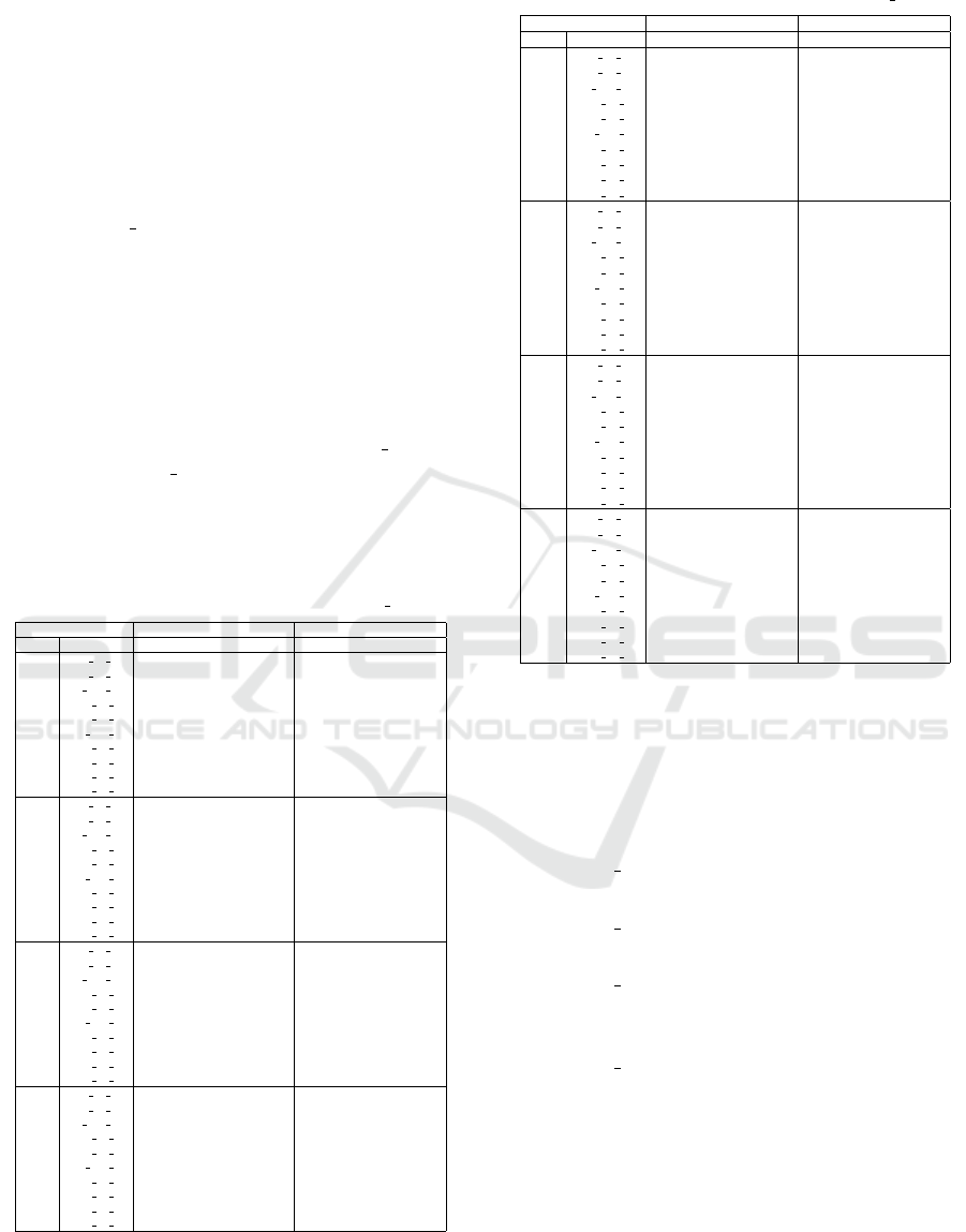
Table 2: MILPI Vs MILPII using PARAM 1.

Instances MILP I MILP II

Bα% Name Nd Gap TT Nd Gap TT

B100%

25 12 1 1 0,00 2,4 1 0,00 7,2

25 36 3 1 0,00 9,9 1 0,00 3,1

25 120 10 6253 0,00 234,3 1 0,00 13,1

100 12 1 236 0,00 34,9 1 0,00 4,4

100 36 3 5925 0,00 305,8 3 0,00 23

100 120 10 6265 0,00 907,5 1 0,00 68,9

250 12 1 6406 0,00 287,5 1 0,00 116,1

250 36 3 6654 0,00 837,57 7 0,00 67,9

500 12 1 6367 0,00 1009,2 135 0,00 134,3

500 36 3 9310 116,2 3 600 131 0,00 194,1

B75%

25 12 1 1 0,00 4,9 1 0,00 3,5

25 36 3 621010 0,003 3 600 2178275 0,002 3600

25 120 10 1 0,00 1,7 1 0,00 1,2

100 12 1 38263 0,00 92,8 14296 0,00 26,9

100 36 3 188045 0,003 3600 1530152 0,001 3600

100 120 10 5387 0,00 43,5 3246 0,00 19,1

250 12 1 1480 0,00 136,8 986 0,00 72,5

250 36 3 44798 0,002 3600 53548 0,00 3600

500 12 1 9429 0,00 611,4 38889 0,00 982

500 36 3 5926 0,2 3600 24416 0,8 3600

B50%

25 12 1 9 0,00 4,3 1 0,00 10,2

25 36 3 5517 0,00 36,7 190069 0,00 125,2

25 120 10 1 0,00 1,7 1 0,00 1,2

100 12 1 9167 0,00 29 2655 0,00 19,8

100 36 3 226990 0,002 3600 900624 0,001 3600

100 120 10 1 0,00 22,7 1 0,00 11,5

250 12 1 67917 0,00 652,6 43693 0,00 211,2

250 36 3 126391 0,00 3600 74672 0,00 915,7

500 12 1 36106 0,00 1 371,2 47726 0,00 1 411

500 36 3 12005 0,01 3600 10404 0,37 3600

B25%

25 12 1 2235 0,00 7,2 1268 0,00 92,6

25 36 3 8723 0,00 40,3 25405 0,00 21,7

25 120 10 1 0,00 1,7 1 0,00 1,2

100 12 1 9038 0,00 25,8 642 0,00 17,5

100 36 3 188045 0,003 3600 1530152 0,001 3600

100 120 10 116 0,00 19,8 29 0,00 9,4

250 12 1 3508340 0,0001 3600 3531930 0,0001 3600

250 36 3 70612 0,001 3600 76767 0,001 3600

500 12 1 7496 0,00 433,5 15472 0,00 307,2

500 36 3 17990 0,003 3600 14637 0,005 3600

Table 3: MILPI Vs MILPII using PARAM 2.

Instances MILP I MILP II

Bα% Name Nd Gap TT Nd Gap TT

B100%

25 12 1 1 0,00 103,8 1 0,00 270,5

25 36 3 1 0,00 2,2 1 0,00 1,7

25 120 10 1 0,00 8,3 1 0,00 4,3

100 12 1 1 0,00 3,8 1 0,00 1,7

100 36 3 1 0,00 8,8 1 0,00 5,3

100 120 10 1 0,00 37,7 1 0,00 23,1

250 12 1 1 0,00 9,3 1 0,00 4,6

250 36 3 1 0,00 30,8 1 0,00 14,9

500 12 1 1 0,00 24,4 1 0,00 10,4

500 36 3 1 0,00 79,7 3 0,00 40,5

B75%

25 12 1 1 0,00 292,9 1 0,00 0,8

25 36 3 105355 0,00 177,1 149396 0,00 86,7

25 120 10 1 0,00 1,7 1 0,00 1,2

100 12 1 1178 0,00 11,9 35 0,00 4,7

100 36 3 12042 0,00 155,2 18610 0,00 82,8

100 120 10 1 0,00 13,1 1 0,00 7,4

250 12 1 1005 0,00 45,7 312 0,00 14,2

250 36 3 6575 0,00 556,7 5432 0,00 97,3

500 12 1 6650 0,00 329,2 5671 0,00 98,8

500 36 3 50874 0,07 3600 75729 0,06 3600

B50%

25 12 1 1 0,00 290,1 1 0,00 0,7

25 36 3 73738 0,00 180,2 67812 0,00 33,6

25 120 10 1 0,00 1,7 1 0,00 1,2

100 12 1 61 0,00 11,1 46 0,00 4,1

100 36 3 20017 0,00 235,9 12837 0,00 84,9

100 120 10 13 0,00 16,7 1 0,00 7,4

250 12 1 5459 0,00 106,7 5430 0,00 33,4

250 36 3 8352 0,00 224,8 617 0,00 35,2

500 12 1 5609 0,00 258,4 362291 0,00 1 970,7

500 36 3 40163 0,00 2 868,1 43120 0,00 1 990,3

B25%

25 12 1 1159 0,00 68,6 761 0,00 41,8

25 36 3 8903 0,00 28,3 8132 0,00 7,3

25 120 10 1 0,00 1,7 1 0,00 1,2

100 12 1 1 0,00 4,5 5 0,00 3,9

100 36 3 25023 0,00 233,9 8548 0,00 57,5

100 120 10 1 0,00 11,2 1 0,00 7,2

250 12 1 6416 0,00 95,3 319 0,00 13,5

250 36 3 6301 0,00 267,3 9614 0,00 118,3

500 12 1 6360 0,00 215,3 13762 0,00 104,3

500 36 3 5652 0,00 754,2 29215 0,00 2390,9

6.2 Numerical Results

In Tables 2-5, we present a comparison between our

two MILP using different parameterizations related to

the values of q

z,0

and ¯q

for zone Z. The parameteri-

zations are deﬁned as follows:

• PARAM 1: q

z,0

= 0% and maximum investment

rate ¯q

is unbounded for all zones,

• PARAM 2: q

z,0

= 0 and ¯q

is bounded for all

zones, as speciﬁed in inequalities (

4),

• PARAM 3: q

z,0

≥ 5% for certain zones and ¯q

bounded for all zones, as indicated in inequalities

(

4),

• PARAM 4: q

z,0

≥ 5% for certain zones, with ¯q

max

for all zones.

We report 3 criteria in the computational study:

• the number of nodes in the B&C tree (Nd),

• the optimality gap (Gap), given in %, which rep-

resents the relative error between the lower bound

and best upper bound obtained at the end of the

resolution,

• the total CPU time computation (TT), given in

seconds.

ICORES 2025 - 14th International Conference on Operations Research and Enterprise Systems

142

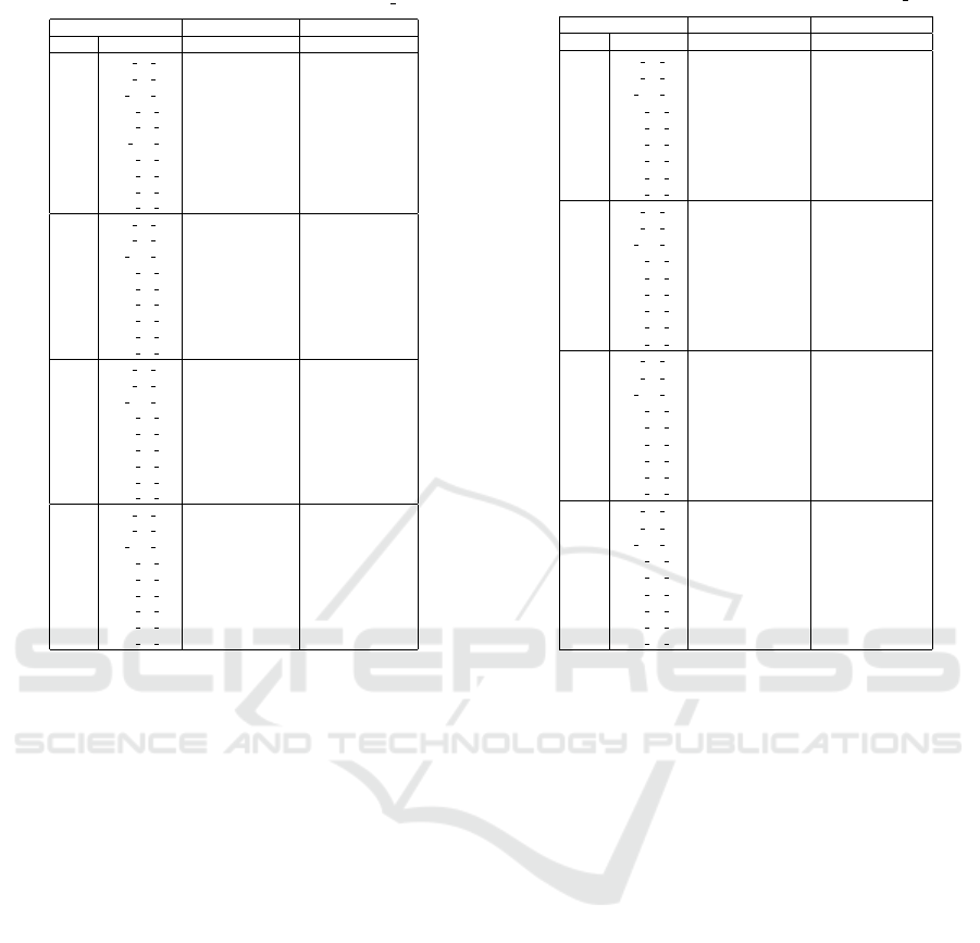
Table 4: MILPI Vs MILPII using PARAM 3.

Instances MILP I MILP II

Bα% Name Nd Gap TT Nd Gap TT

B100%

25 12 1 1 0,00 0,2 1 0,00 0,2

25 36 3 1 0,00 0,9 1 0,00 0,5

25 120 10 1 0,00 2,7 1 0,00 1,5

100 12 1 1 0,00 1,2 1 0,00 1,2

100 36 3 1 0,00 3,6 1 0,00 1,9

100 120 10 1 0,00 1 0,00 7,6

250 12 1 1 0,00 2,9 1 0,00 1,6

250 36 3 1 0,00 9,9 1 0,00 5,5

500 12 1 1 0,00 6,2 1 0,00 3,3

500 36 3 1 0,00 17,9 1 0,00 11,1

B75%

25 12 1 1 0,00 0,2 1 0,00 0,2

25 36 3 1 0,00 0,9 1 0,00 0,5

25 120 10 1 0,00 3,5 1 0,00 3,2

100 12 1 1 0,00 1,2 1 0,00 0,6

100 36 3 1 0,00 3,1 1 0,00 1,8

250 12 1 1 0,00 2,9 1 0,00 1,6

250 36 3 1 0,00 10,3 1 0,00 5,6

500 12 1 1 0,00 6,2 1 0,00 3,2

500 36 3 1 0,00 20,7 1 0,00 11

B50%

25 12 1 1 0,00 0,2 1 0,00 0,2

25 36 3 1 0,00 0,9 1 0,00 0,5

25 120 10 1 0,00 3,3 1 0,00 1,5

100 12 1 1 0,00 1,2 1 0,00 0,6

100 36 3 1 0,00 3,6 1 0,00 1,9

250 12 1 1 0,00 2,7 1 0,00 1,6

250 36 3 1 0,00 10,1 1 0,00 5,6

500 12 1 1 0,00 6,4 1 0,00 3,2

500 36 3 1 0,00 20,7 1 0,00 10,5

B25%

25 12 1 1 0,00 0,2 1 0,00 0,2

25 36 3 1 0,00 0,9 1 0,00 0,5

25 120 10 1 0,00 3,5 1 0,00 1,5

100 12 1 1 0,00 1,2 1 0,00 0,6

100 36 3 1 0,00 3,6 1 0,00 1,9

250 12 1 1 0,00 2,9 1 0,00 1,6

250 36 3 1 0,00 9,9 1 0,00 5,1

500 12 1 1 0,00 6,3 1 0,00 3,2

500 36 3 1 0,00 20,5 1 0,00 11

The results indicate that our two mixed integer linear

programs exhibit excellent performance, successfully

solving nearly all instances to optimality within just

a few minutes. For this, 94.1% (resp. 92.2%) of in-

stances are solved to optimality by the second (resp.

ﬁrst) formulation. Furthermore, the second formu-

lation yields better results for 50% of instances that

remain unsolved to optimality by both formulations.

It also successfully solves several instances to opti-

mality that the ﬁrst formulation does not. Regard-

ing the CPU time computation, the second formula-

tion signiﬁcantly outperforms the ﬁrst, achieving so-

lutions in shorter CPU times for 85.62% of instances.

We observe also that 68.62% (resp. 40.10%) of in-

stances are solved to optimality in under 15 seconds

by the second (resp. ﬁrst) formulation. On the other

hand, the branching tree associated with the Branch-

and-Cut algorithm when using the second formula-

tion shows a reduced number of nodes for 24.18% in-

stances compared to the ﬁrst formulation. Also, the

second formulation solves 3.27% of instances to op-

timality at the root of the branching tree, while the

ﬁrst formulation requires more nodes for the same

instances (i.e., branching is required to achieve op-

timal solutions). This clearly shows the advantages

of the second formulation in effectively solving the

problem. Additionally, we observed that the problem

Table 5: MILPI Vs MILPII using PARAM 4.

Instances MILP I MILP II

Bα% Name Nd Gap TT Nd Gap TT

B100%

25 12 1 1 0,00 0,3 1 0,00 0,2

25 36 3 1 0,00 0,5 1 0,00 0,5

25 120 10 1 0,00 1,9 1 0,00 1,8

100 12 1 1 0,00 1,3 1 0,00 0,9

100 36 3 1 0,00 3,2 1 0,00 2,1

250 12 1 1 0,00 2,9 1 0,00 1,7

250 36 3 1 0,00 6,2 1 0,00 5,7

500 12 1 1 0,00 6,2 1 0,00 3,5

500 36 3 1 0,00 12,2 1 0,00 11,7

B75%

25 12 1 1 0,00 0,3 1 0,00 0,2

25 36 3 1 0,00 1 1 0,00 0,5

25 120 10 1 0,00 2,6 1 0,00 2,1

100 12 1 1 0,00 1,3 1 0,00 0,8

100 36 3 1 0,00 2,6 1 0,00 2

250 12 1 1 0,00 3 1 0,00 1,7

250 36 3 1 0,00 6,3 1 0,00 5,8

500 12 1 1 0,00 6,3 1 0,00 3,5

500 36 3 1 0,00 11,8 1 0,00 11,6

B50%

25 12 1 1 0,00 0,3 1 0,00 0,2

25 36 3 1 0,00 0,9 1 0,00 0,5

25 120 10 1 0,00 2,4 1 0,00 1,9

100 12 1 1 0,00 1,1 1 0,00 1

100 36 3 1 0,00 3,4 1 0,00 2

250 12 1 1 0,00 3 1 0,00 1,7

250 36 3 1 0,00 6 1 0,00 5,6

500 12 1 1 0,00 6,3 1 0,00 3,5

500 36 3 1 0,00 11,9 1 0,00 11,6

B25%

25 12 1 1 0,00 0,3 1 0,00 0,2

25 36 3 1 0,00 0,9 1 0,00 0,5

25 120 10 1 0,00 2,4 1 0,00 1,9

100 12 1 1 0,00 1,1 1 0,00 0,9

100 36 3 1 0,00 3,5 1 0,00 2,1

250 12 1 1 0,00 2,9 1 0,00 1,7

250 36 3 1 0,00 5,9 1 0,00 5,6

500 12 1 1 0,00 6,4 1 0,00 3,5

500 36 3 1 0,00 12,4 1 0,00 11,6

becomes increasingly complex to solve to optimality

when the parameter q

z,0

is set to zero, and the in-

equalities in (

4) are relaxed for all zones in Z. This

complexity arises from the combinatorial nature of

the problem, resulting in a signiﬁcant increase in the

number of potential feasible solutions.

Since nearly all instances have been solved to opti-

mality, we cannot assess the impact of our additional

valid inequalities on the B&C algorithm’s effective-

ness. This limits our evaluation of their inﬂuence on

solution times and overall performance. We need to

generate more complex instances that challenge op-

timal solutions with our formulations. Further com-

putational studies are essential to determine how our

valid inequalities can accelerate solution times for in-

stances solved to optimality without them.

7 CONCLUSION

In this paper, we have addressed the strategic deci-

sion problem of a telecommunication operator which

aims at efﬁciently planning its future investments in

Fiber access of geographical areas that are currently

undeployed. We have introduced two mixed integer

linear programs to model the problem. Additionally,

we presented several classes of valid inequalities for

Models and Algorithms for the Optimization of Multi-Period Fiber Wholesale Investments Strategies

143

the associated polytopes. These results are used to

develop a Branch-and-Cut algorithm for solving the

problem. An extensive computational study was con-

ducted to assess the algorithm’s performance across

various instances and scenarios. While our approach

has proven effective, it would be beneﬁcial to investi-

gate the impact of our valid inequalities in the context

of larger and more complex instances. Such an analy-

sis could yield valuable insights into the strengths and

weaknesses of both approaches.

ACKNOWLEDGEMENTS

We would like to acknowledge the contribution of the

Orange Wholesale France team members who have

contributed to this study and preparation of the real

data for our computational study. We are grateful for

their expertise in making this work possible.

REFERENCES

Angilella, V., Chardy, M., and Ben-Ameur, W. (2016).

Cables network design optimization for the ﬁber to

the home. In 12th International Conference on the

Design of Reliable Communication Networks, DRCN

2016, Paris, France, March 15-17, 2016, pages 87–

94. IEEE.

Angilella, V., Chardy, M., and Ben-Ameur, W. (2018). Fiber

cable network design with operations administration

& maintenance constraints. In Parlier, G. H., Liber-

atore, F., and Demange, M., editors, Proceedings of

the 7th International Conference on Operations Re-

search and Enterprise Systems, ICORES 2018, Fun-

chal, Madeira - Portugal, January 24-26, 2018, pages

94–105. SciTePress.

Cambier, A., Chardy, M., Figueiredo, R., Ouorou, A., and

Poss, M. (2021). Optimizing the investments in mo-

bile networks and subscriber migrations for a telecom-

munication operator. Networks, 77(4):495–519.

Chardy, M., Costa, M., Faye, A., and Trampont, M.

(2012). Optimizing splitter and ﬁber location in a

multilevel optical FTTH network. Eur. J. Oper. Res.,

222(3):430–440.

Cook, S. A. (1971). The complexity of theorem-proving

procedures. In Proceedings of the Third Annual ACM

Symposium on Theory of Computing, STOC ’71, page

151–158, New York, NY, USA. Association for Com-

puting Machinery.

Dgtlinfra (2021). https://dgtlinfra.com/broadband-

investment-deployment-government-funding/.

Farah, S. and Andresen, G. B. (2024). Investment-based

optimisation of energy storage design parameters in a

grid-connected hybrid renewable energy system. Ap-

plied Energy, 355:122384.

Faria, V. A., Rodrigo de Queiroz, A., and DeCarolis, J. F.

(2023). Scenario generation and risk-averse stochastic

portfolio optimization applied to offshore renewable

energy technologies. Energy, 270:126946.

Gao, C., Wang, X., Li, D., Han, C., You, W., and Zhao,

Y. (2023). A novel hybrid power-grid investment op-

timization model with collaborative consideration of

risk and beneﬁt. Energies, 16(20).

Gao, L., Zhao, Z.-Y., and Li, C. (2022). An investment

decision-making approach for power grid projects: A

multi-objective optimization model. Energies, 15(3).

Giannelos, S., Borozan, S., Aunedi, M., Zhang, X., Ameli,

H., Pudjianto, D., Konstantelos, I., and Strbac, G.

(2023). Modelling smart grid technologies in optimi-

sation problems for electricity grids. Energies, 16(13).

otschel, M., Lov

asz, L., and Schrijver, A. (1988). Sta-

ble Sets in Graphs, pages 272–303. Springer Berlin

Heidelberg, Berlin, Heidelberg.

otschel, M., Raack, C., and Werner, A. (2014). To-

wards optimizing the deployment of optical access

networks. EURO Journal on Computational Opti-

mization, 2(1):17–53.

He, Y., Liao, N., Rao, J., Fu, F., and Chen, Z. (2019). The

optimization of investment strategy for resource uti-

lization and energy conservation in iron mines based

on monte carlo and intelligent computation. Journal

of Cleaner Production, 232:672–691.

Hervet, C., Chardy, M., Costa, M.-C., Faye, A., and Franc-

fort, S. (2012). Robust optimization of optical ﬁber

access networks deployments. In International Sym-

posium on Mathematical Programming (ISMP 2012)

(and EURO 2012, Vilnius, Lithuania), page 1, Berlin,

Germany.

Kerdphol, T., Qudaih, Y., and Mitani, Y. (2016). Optimum

battery energy storage system using pso considering

dynamic demand response for microgrids. Interna-

tional Journal of Electrical Power & Energy Systems,

83:58–66.

Nemhauser, G. and Sigismondi, G. (1992). A strong

cutting plane/branch-and-bound algorithm for node

packing. Journal of the Operational Research Soci-

ety, 43(5):443–457.

Nemhauser, G. and Wolsey, L. (1988). The Theory of Valid

Inequalities, chapter II.1, pages 203–258. John Wiley

& Sons, Ltd.

Schrijver, A. (1986). Theory of linear and integer program-

ming. In Wiley-Interscience series in discrete mathe-

matics and optimization.

Silva, I. F., Bentz, C., Bouhtou, M., Chardy, M., and Kedad-

Sidhoum, S. (2024). Optimization of battery manage-

ment in telecommunications networks under energy

market incentives. Ann. Oper. Res., 332(1):949–988.

Tuballa, M. L. and Abundo, M. L. (2016). A review of the

development of smart grid technologies. Renewable

and Sustainable Energy Reviews, 59:710–725.

Wang, Y., Ma, Y., Song, F., Ma, Y., Qi, C., Huang, F.,

Xing, J., and Zhang, F. (2020). Economic and efﬁ-

cient multi-objective operation optimization of inte-

grated energy system considering electro-thermal de-

mand response. Energy, 205:118022.

ICORES 2025 - 14th International Conference on Operations Research and Enterprise Systems

144

Zafar, R., Mahmood, A., Razzaq, S., Ali, W., Naeem, U.,

and Shehzad, K. (2018). Prosumer based energy man-

agement and sharing in smart grid. Renewable and

Sustainable Energy Reviews, 82:1675–1684.

Zappal

a, P., Benhamiche, A., Chardy, M., Pellegrini, F. D.,

and Figueiredo, R. (2022). A timing game approach

for the roll-out of new mobile technologies. In 20th

International Symposium on Modeling and Optimiza-

tion in Mobile, Ad hoc, and Wireless Networks, WiOpt

2022, Torino, Italy, September 19-23, 2022, pages

217–224. IEEE.

Zhang, Q., Xia, L., and He, W. (2019). The optimization

research of investment management in power grid en-

terprise. IOP Conference Series: Earth and Environ-

mental Science, 332(4):042016.

Models and Algorithms for the Optimization of Multi-Period Fiber Wholesale Investments Strategies

145