Next-Generation Design Tools for Intelligent Transportation Systems

Dominik Ascher

and Georg Hackenberg

Faculty of Electrical Engineering and Computer Science, Technical University of Berlin, 10587 Berlin, Germany

School of Engineering, University of Applied Sciences Upper Austria, Stelzhamerstraße 23, 4600 Wels, Austria

Keywords:

Model- and Simulation-Based Systems Engineering, Model-Based Design, Intelligent Transportation

Systems.

Abstract:

Intelligent Transportation Systems (ITS) promote new transportation paradigms such as connected and au-

tonomous vehicles (CAV), multi-modal and demand-responsive transport systems, and enable the transporta-

tion electriﬁcation by sustainable operation of electric vehicles. Methods and tools are needed to explore the

possible design space for emerging transportation paradigms, which support evaluation of system design alter-

natives and veriﬁcation of system properties. In this work, we propose a model- and simulation-based systems

engineering framework for capturing design decisions and evaluating control strategies for ITS design. In

addition to capturing and evaluating different design decisions, the proposed solution allows users to guide

design decisions by systematic comparison and evaluation of system conﬁgurations and control strategies.

1 INTRODUCTION

The transformative patterns of future mobility are en-

abled by interconnected as well as integrated sys-

tems and services. For this, Intelligent Transportation

Systems (ITS) establish new transportation paradigms

such as connected and autonomous vehicles (CAV)

(Kopelias et al., 2020), multi-modal and demand-

responsive transport systems (Brake et al., 2004), as

well as the transportation electriﬁcation by sustain-

able operation of electric vehicles (Zhang and Fuji-

mori, 2020). In order to minimize environmental im-

pacts, complex scenarios between these systems and

their requirements need to be holistically addressed,

from which integrated system designs are derived,

which enable transportation infrastructure and het-

erogenous actor efﬁciency and sustainability.

To systematically support the aforementioned sys-

tems engineering task, model- and simulation-based

systems engineering (Gianni et al., 2014) can be em-

ployed for abstraction of design problems through the

formulation of system models and their evaluation in

terms of concrete behavior at run time, where simu-

lation aids projecting run-time information and per-

formance metrics about the system under design and

environment. However, as systems and their under-

lying requirements are typically imperfectly under-

stood at the beginning of the design task, methods and

tools are needed to explore the possible design space

for emerging transportation paradigms, which support

evaluation of system design alternatives and veriﬁca-

tion of system properties.

With our research, we want to help improve the

efﬁciency, effectiveness and sustainability of today’s

transportation systems. To achieve this goal, we work

on methodologies for designing such systems and ver-

ifying their properties. Fundamentally, we promote a

formal approach capturing the relevant design deci-

sions and their relations. Furthermore, we integrate

scenario-based simulation of system dynamics and

evaluation of emergent properties. Finally, we ex-

ploit optimization algorithms for optimizing system

dynamics as well as static design decisions.

In this paper, we explore how the next gener-

ation of design tools for ITS addressing emerging

paradigms could look like. Therefore, ﬁrst we want

to understand which system properties and design de-

cisions should be represented in these tools. Then, we

want to learn how design decisions could be veriﬁed

with respect to the desired system properties. Finally,

we want to study how the relevant design information

could be represented in a graphical user interface.

In the following, we ﬁrst describe an overview of

related work for our approach in Section 2. Then,

we describe approach and methodology for a model-

and simulation-based systems engineering framework

for capturing and evaluating design decisions in Sec-

tion 3. Thereafter, we describe a tool prototype for

building system designs, conducting simulation runs,

and visualizing simulation outcomes in Section 4.

234

Ascher, D. and Hackenberg, G.

Next-Generation Design Tools for Intelligent Transportation Systems.

DOI: 10.5220/0013183200003896

Paper published under CC license (CC BY-NC-ND 4.0)

In Proceedings of the 13th International Conference on Model-Based Software and Systems Engineering (MODELSWARD 2025), pages 234-241

ISBN: 978-989-758-729-0; ISSN: 2184-4348

2 RELATED WORK

We discuss related work for ITS in terms of infras-

tructure planning, eco-routing and driving, coopera-

tive driving as well as mobility-on-demand systems.

Infrastructure Planning. Trafﬁc simulation tools

such as PTV Vissim (Fellendorf, 1994), MATSim

(W Axhausen et al., 2016), SUMO (Lopez et al.,

2018) as well as AIMSUN (Barcel

o and Casas, 2005)

support analysis and decision-making for transporta-

tion systems engineering problems. For instance,

SUMO can be used to assess mesoscopic to micro-

scopic trafﬁc scenarios, based on behavior models

for passenger and vehicle behavior, and infrastruc-

ture models separating links, intersections and lanes

for different transport modalities, while implement-

ing actor and trafﬁc control strategies.

Eco-Routing and -Driving. Eco-routing (Ericsson

et al., 2006) describes a concept, which focuses on

trafﬁc participants and their routes in terms of tar-

geting energy-efﬁcient route selection and reduction

of emissions, whereas the concept of Eco-Driving

(Huang et al., 2018) focuses on energy-efﬁcient in-

termediate driving behavior. Potential congestions

may arise within transport networks of single modali-

ties due to their excessive utilization, where energy-

efﬁcient utilization of different transport modalities

can be targeted (Namoun et al., 2021).

Cooperative Driving. Cooperative driving of in-

telligent connected vehicles (Wang et al., 2022) is

enabled by Vehicle-to-Vehicle (V2V), Vehicle-to-

Infrastructure (V2I) or Vehicle-to-Everything (V2X)

communication. Speciﬁc use-cases include vehicle

platooning (Jia et al., 2015), management of dis-

tributed electric vehicle ﬂeets and their integration to

stabilize ancillary systems such as the power grid in

the context of Vehicle-to-Grid (V2G) (Hu et al., 2016)

applications, as well as alignment of different trans-

portation modalities (Harris et al., 2015).

Mobility-on-Demand. Mobility-on-demand sys-

tems refer to systems, where transportation demands

get covered by transportation modalities, which

make up the transportation supply. Here, Rideshar-

ing favors shared mobility over personal mobility,

bringing together passengers with a shared route

in shared vehicles (Furuhata et al., 2013). In au-

tonomous mobility-on-demand systems, autonomous

transportation modalities cover transportation supply

while increasing system efﬁciency (Fagnant and

Kockelman, 2014).

3 METHODOLOGY AND

APPROACH

Our model- and simulation-based systems engineer-

ing approach is based on (Ascher and Hackenberg,

2015; Ascher and Hackenberg, 2016; Ascher and

Hackenberg, 2017; Ascher et al., 2023; Ascher and

Hackenberg, 2023) and employs an integrated sys-

tems modeling technique for design of integrated ITS

systems and investigation of emergent system prop-

erties. Our modeling technique supports both static

property, i.e. structural and infrastructure design, and

dynamic property design, i.e. behavior and control

strategy design. Here, Figure 1 shows an overview of

the system design methodology.

Figure 1: System design methodology.

Subsequently, ﬁrst the intended usage of the

framework is described in Section 3.1. Secondly,

domain-speciﬁc design concepts for the framework

are described in Section 3.2. Thirdly, problem solu-

tion for design problems is described in Section 3.3.

3.1 Intended Usage

We subsequently describe use-cases considering dif-

ferent roles for our systems engineering approach for

investigation of static and dynamic properties:

Transportation System Engineers (TSEs). main-

tain and design transportation infrastructure.

• Static Properties: TSEs may be supported in the

investigation of transportation infrastructure prop-

erties such as placement of intersections and links,

and capacities of links such as number of lanes.

• Dynamic Properties: TSEs may be supported in

devising trafﬁc control strategies and semaphores

incorporating demand-responsive cycle times.

Charge Point Operators (CPOs). maintain and

operate a charging infrastructure in a deﬁned area.

• Static Properties: CPOs may be supported in de-

vising charging infrastructure such as planning of

placement and capacity of charging stations along

most frequented routes and points of interest.

Next-Generation Design Tools for Intelligent Transportation Systems

235

• Dynamic Properties: CPOs may be supported in

charging scheduling and coordination during peak

demand and renewable energy supply times.

Mobility Feet Operators (MFOs). coordinate and

manage a ﬂeet of vehicles serving demands.

• Static Properties: MFOs may be supported in de-

termination of ﬂeet capacity as well as planning

of vehicle types and modalities to be utilized.

• Dynamic Properties: MFOs may be supported in

determining routing and driving decisions for mo-

bility ﬂeets with respect to underlying goals such

as energy-efﬁciency or shortest traveling or wait-

ing times while serving transportation demands.

3.2 System Theory

The approach allows domain-speciﬁc modeling of

integrated transportation system problems on meso-

scopic to microscopic levels. Figure 2 depicts

domain-speciﬁc modeling concepts. Subsequently,

we provide a brief overview of domain concepts,

states, as well as events, where we refer to (Ascher

and Hackenberg, 2023) for a detailed overview.

Figure 2: Domain-speciﬁc modeling concepts.

Concepts. The formalism deﬁnes intersections i ∈

I, segments s ∈ S as well as locations l ∈ L for de-

scribing properties about the transportation infras-

tructure. Based on the transportation infrastructure,

we use charging stations cs ∈ CS for describing the

charging infrastructure. Furthermore, we use vehicles

v ∈ V to describe the transportation supply and ca-

pacities. Transportation demands d ∈ D are based on

the transportation infrastructure, and temporarily con-

sume transportation capacities such as vehicles.

States. Based on the concepts, we describe dynamic

(i.e. time-dependent) state functions for charging sta-

tions S

, demands S

, as well as vehicles S

• In terms of charging station states S

, we de-

scribe the current vehicle which is connected to

the charging station S

CS.CV

, as well as the current

charge speed S

CS.CCS

• In terms of demand states S

, we describe the cur-

rent vehicle carrying the demand S

D.CV

, as well as

the current location of the demand S

D.CL

• For vehicle states S

, we describe the current

battery level of the vehicle S

V.CBL

, the current lo-

cation of the vehicle S

V.CL

, as well as the current

drive speed of the vehicle S

V.CDS

Events. We deﬁne the following domain-speciﬁc

events E:

• Events indicating vehicle arrival at intersections

V.AI

or vehicle departure at intersections E

V.DI

derive routing decisions.

• Events indicating vehicle arrival at charging sta-

tions E

V.ACS

to derive charging decisions.

• Events indicating vehicle arrival at demand pick-

up locations E

V.ADP

and at drop-off locations

V.ADD

to derive pick-up and drop-off decisions.

• Events indicating faster vehicle arrival at slower

vehicles E

V.AV S

, as well as faster vehicle departure

at slower vehicles E

V.DV S

to derive overtaking de-

cisions on the same segment.

• Events indicating demand appearance E

D.AD

derive decisions for vehicles to serve demands.

• Events indicating vehicle drive speed change

V.CDS

and charge speed change E

V.CCS

to derive

decisions for overtaking and charging behaviors.

• Events indicating vehicle batteries becoming

empty E

V.CBE

or full E

V.CBF

to derive decisions

for stopping driving and charging behaviors.

3.3 Problem Solution

For solving according design problems, Dynamic

Programming (DP) (Bellman, 1957) methods can be

employed for small-scale problems by iteratively ex-

ploring the state space over a deﬁned time horizon to

ﬁnd an optimal solution, but are subject to increas-

ing problem complexity with increasing dimension-

ality of parameter, state and action spaces, i.e. the

curse of dimensionality (Bellman, 1957), restricting

their applicability. To reduce simulation and decision

making complexity, we apply the following methods:

Monte-Carlo Simulation. methods are used,

which partially and/or randomly sample the state

space until an sufﬁcient number of samples is reached

for exploration to limit problem complexity (Ascher

and Hackenberg, 2015).

MODELSWARD 2025 - 13th International Conference on Model-Based Software and Systems Engineering

236

Discrete-Event Simulation. is used, where events

are deﬁned as functions over a system’s trajectory of

states, which indicate when actions need to be taken in

the system simulation, thereby reducing action space

dimensionality (Ascher and Hackenberg, 2023).

Heuristic Search. procedures are employed, which

are iteratively designed by domain experts, where

simulation results are utilized to adapt heuristic con-

trol logic as needed (Ascher and Hackenberg, 2015).

Approximate Dynamic Programming. methods

employ approximations of policy and value functions

(Powell, 2007), which are used to reduce DP problem

complexity (Ascher et al., 2023).

4 TOOL PROTOTYPE

Based on the general approach explained in Section 3

we started developing an open source tool prototype

hosted on GitHub

, which we subsequently describe:

In Section 4.1 we describe core data structures for

representing both static system conﬁgurations and dy-

namic system states. Then, in Section 4.2 we explain

how users can implement and integrate different con-

trol strategies into the tool prototype. Next, in Sec-

tion 4.3 we describe data collected during simulation

runs which can be used for visualizations and possibly

training. In Section 4.4 we provide an overview of the

engine, which computes discrete events and updates

system states accordingly. Finally, in Section 4.5 we

highlight two different framework applications.

4.1 Data Structures

The model module provides the core data structures

for modeling static system conﬁgurations and repre-

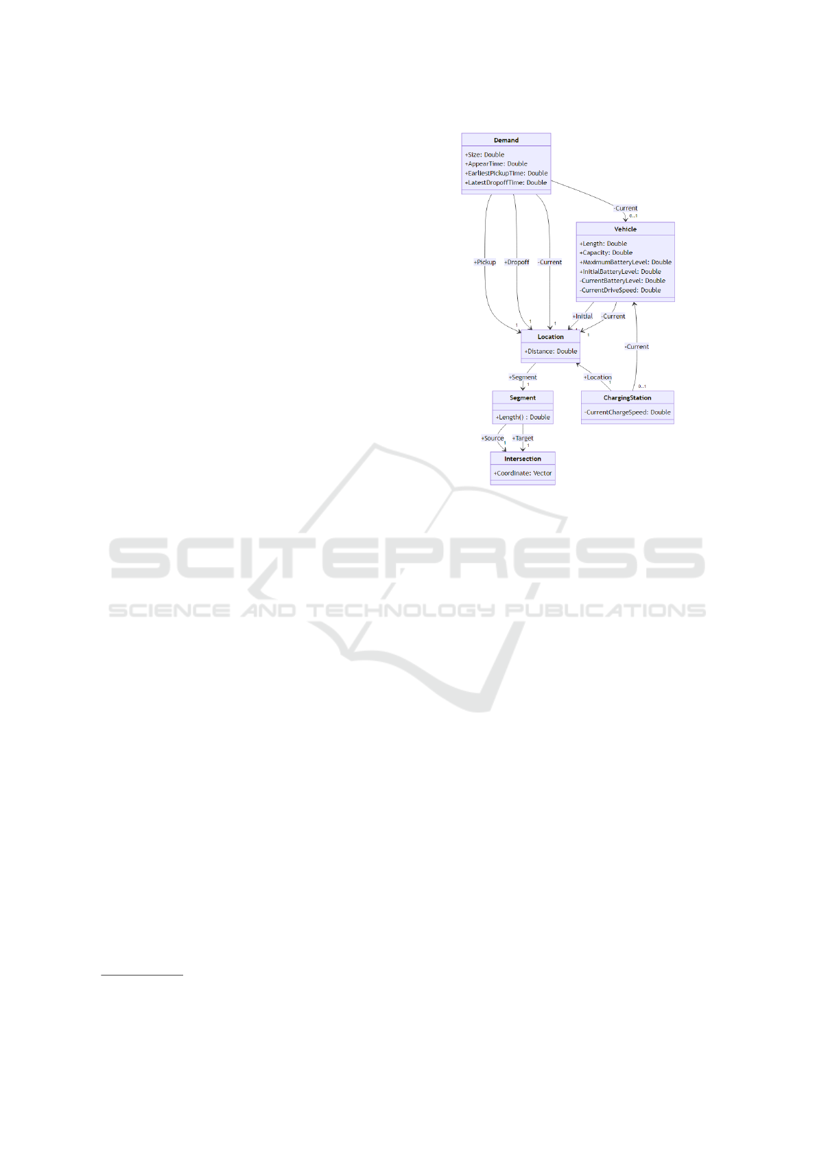
senting dynamic system states. Figure 3 shows the

classes, their attributes, and their relationships.

The Intersection class represents intersections

of the driving infrastructure. Each intersection stores

its coordinate in three-dimensional space. Note that

we use Cartesian coordinates for simplicity.

The Segment class represents road segments of

the driving infrastructure. Each segment points to its

source and target intersection and provides a method

for computing its length based on Euclidean distance.

The Location class represents speciﬁc points on

the segments of the driving infrastructure, where each

https://github.com/ghackenberg/transport-ide

Figure 3: Conﬁguration and simulation data model.

location points to a corresponding segment. Further-

more, each location stores a distance on this segment

measured in Eclidean units of the Cartesian space.

The ChargingStation class represents the charg-

ing infrastructure. Each charging station stores its

location on the driving infrastructure. Furthermore,

each charging station optionally points to a current

vehicle. Each charging station provides the current

charging speed, where the simulator computes the

current charging speed dynamically.

The Vehicle class represents the driving re-

sources. Each vehicle provides an initial and a cur-

rent location on the driving infrastructure. The initial

location deﬁnes the position of the vehicle in the ini-

tial state of the simulation. Then, the simulator con-

tinuously updates the current location of the vehicle.

Furthermore, each vehicle stores a length and a capac-

ity, a maximum, an initial, and a current battery level,

and a current drive speed. The length determines how

much space the vehicle occupies on the driving infras-

tructure. The capacity deﬁnes how much demand the

vehicle can carry. The maximum battery level spec-

iﬁes the size of the energy storage. The initial bat-

tery level stores the load state of the enery storage at

simulation start. Finally, the simulator continuously

updates current battery level and current drive speed.

The Demand class represents the transportation

loads to be served. Each demand points to a pickup

and a dropoff location as well as a current location

Next-Generation Design Tools for Intelligent Transportation Systems

237

and vehicle. Furthermore, each demand stores a size

as well as an appear, and earliest pickup, and a latest

dropoff time. The simulator continuously updates the

current location and vehicle.

4.2 Control Strategies

During a simulation run, a number of control deci-

sions have to be taken. For example, when arriving

at an intersection each vehicle has to select the next

outgoing road segment. Similarly, when arriving at

a demand pickup location each vehicle as to decide

whether to serve the demand or not. The overall sys-

tem performance heavily depends on the optimality

of the individual choices made during a simulation

run. Therefore, one key engineering task for this class

of systems is to develop an appropriate control strat-

egy. Since desired control strategies cannot be hard-

coded upfront, the simulator supports plugging in and

testing different strategies, which must implement the

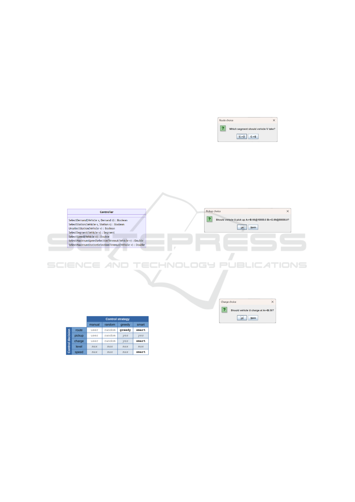
controller interface methods depicted in Figure 4.

Figure 4: Methods of the controller interface.

We currently provide four different implementa-

tions of the controller interface: A manual, a ran-

dom, a greedy, and a smart control strategy. Figure 5

provides an overview of the four control strategies and

their decision logic. Columns of the matrix represent

individual control strategies, rows represent decisions

to be taken, and cells represent corresponding logic.

Figure 5: Overview of the control strategies.

In the following, we describe the logics behind

each of the control strategies in more detail.

4.2.1 Manual Control Strategy

The manual control strategy delegates routing, de-

mand pickup, and charge decisions to the tool user

using input dialogs. The remaining control decisions

are derived automatically.

Figure 6 shows the input dialog for route deci-

sions, which pops upon vehicle arrival at an intersec-

tion. It provides the vehicle name (V in the example)

and possible follow-up road segments (C->D and C->E

in the example). Note that C, D, and E represent the

intersection names connected through segments. The

user can select the desired routing option by pressing

the button for the respective follow-up segment.

Figure 6: Vehicle route choice.

Figure 7 shows the input dialog for demand

pickup decisions, which pops up when a vehicle ar-

rives at the pickup location of an appeared and un-

served demand. It provides the vehicle name (U in the

example), demand data (i.e. pickup location, earliest

pickup time, dropoff location as well as latest dropoff

time), and two choice buttons (i.e. yes and no).

Figure 7: Demand pickup choice.

Figure 8 shows the input dialog for vehicle charg-

ing decisions, which pops up when a vehicle arrives

at the location of an unoccupied charging station. The

dialog provides the name of the vehicle (U in the ex-

ample), the location of the charging station (A->B:50

in the example), and the buttons for the two avail-

able choices (i.e. yes and no). Finally, the strategy al-

Figure 8: Vehicle charging choice.

ways selects the maximum driving speed for each ve-

hicle without considering possible collisions and al-

ways chooses to fully charge vehicle batteries after

the user decided to start the charging process.

4.2.2 Random Control Strategy

The random control strategy uses a random number

generator for making routing, demand pickup, and

charging decisions. For each decision, it assigns equal

probabilities to available choices (i.e. outgoing seg-

ments of intersections or yes and no). Driving speed

and target battery charge level are handled equally to

the manual control strategy.

MODELSWARD 2025 - 13th International Conference on Model-Based Software and Systems Engineering

238

4.2.3 Greedy Control Strategy

The greedy control strategy determines routing deci-

sions upon vehicle arrival at intersections of the driv-

ing infrastructure. Its logic comprises four rules being

sequentially processed until one rule applies:

1. When the battery of the vehicle is only half full

or less, the strategy randomly selects an outgoing

road segment with charging station if such seg-

ment is available.

2. Then, when the vehicle carries one or more de-

mands, the strategy randomly selects the drop-off

segment of one such demand if reachable directly

via the intersection.

3. Next, when the vehicle carries no demand, the

strategy randomly selects the pick-up segment of

an unserved demand if reachable directly via the

intersection.

4. Finaly, when none of the above three rules apply,

the strategy randomly selects any of the outgoing

road segments of the current intersection with uni-

form probability distribution.

Note that the desribed routing logic only considers

the next segment and does not perform a look-ahead

across more segments. Finally, the greedy control

strategy always chooses to pick up demands or charge

vehicle batteries if arriving at an unserved demand

pick-up location or charging station. The strategy al-

ways chooses to drive at maximum speed and fully

charge batteries if a charging process has started.

4.2.4 Smart Control Strategy

The smart control strategy uses a more sophisticated

strategy for determining routing decisions upon vehi-

cle intersection arrivals. Its logic comprises four rules

being sequentially processed until one rule applies:

1. When the vehicle carries one or more demands

and a charging station can be reached via their

drop-off location, the segment leading to the clos-

est such demand is selected.

2. When the vehicle carries no demands and a charg-

ing station can be reached via the pick-up location

of an unserved demand, the segment leading to the

closest such demand is selected.

3. When the vehicle carries no demands and does not

plan to pick-up a new demand, the segment lead-

ing to the closest charging station is selected if

reachable with the remaining battery level.

4. Finally, when none of the above three rules ap-

ply, again the strategy randomly selects any of the

outgoing road segments of the current intersection

with uniform probability distribution.

When arriving at an unused charging station, this

strategy only starts charging if no other charging sta-

tion can be reached with the current battery level.

When the charging station is occupied, but no other

charging station can be reached, the strategy lets the

vehicle wait at the station to become free. With this

strategy vehicles always pick up unassigned demands

when passing by, charge their batteries fully when at

charging stations, and drive with maximum speed.

4.3 Data Recorder

During simulation, a number of events are recorded

for visualization of system (and control strategy) per-

formance as well as strategy training. Figure 9 shows

the provided methods of the data recorder interface.

Figure 9: Data recorder interface.

The recorder tracks, when a vehicle crosses an in-

tersection, and records associated routing decisions of

the control strategy. It tracks, when a vehicle passes

by an unassigned demand and the control strategy de-

clines or accepts the pick up. Similarly, the recorder

tracks, when a vehicle drops off a demand at its tar-

get location. Furthermore, it continuously tracks the

speed and overall travel distance of vehicles and size

of time steps made during discrete event simulation.

Currently, we use data about intersection crossing

for determining driving infrastructure bottlenecks and

data about pick ups and drop offs for determining per

demand waiting and driving time as well as delays.

4.4 Simulation Engine

The simulation engine computes event times, dele-

gates control decisions to the control strategy, up-

dates model state, and dispatches relevant data to the

recorder. It employs a simulation loop, which ad-

vances the model time and updates the model state

until no more events are to be processed. The simula-

tion loop can be divided into three main steps:

Step 1. Make routing decisions and update vehi-

cle locations. Make charging decisions and update

connections between vehicles and charging stations.

Make pick up decisions, perform drop offs (also if ve-

hicle battery empty), and update connections between

Next-Generation Design Tools for Intelligent Transportation Systems

239

vehicles and demands. Make speed decisions and up-

date vehicle speeds.

Step 2. Compute time of next event to be processed:

Determine speed update timeout, charging speed up-

date or charging station disconnect timeout, intersec-

tion arrival, charging station arrival, vehicle battery

empty/full, demand appearance, demand overdue, de-

mand pick up / drop off location arrival, and vehicle

attach / detach.

Step 3. Based on current time and time until next

event do the following: Update vehicle locations, ve-

hicle battery levels, and record travelled distances of

vehicles. Detect vehicle collisions based on their lo-

cation, width, and overlaps along the segment line.

Finally, set model time to time of next event.

4.5 Speciﬁc Applications

Based on the previous components we implemented

two speciﬁc applications: The ﬁrst application can be

used for comparing the performance of different con-

trol strategies (see Section 4.5.1). The second appli-

cation can be used for comparing the performance of

different driving and charging infrastructures as well

as ﬂeet conﬁgurations (see Section 4.5.2).

4.5.1 Control Strategy Comparison

To compare different control strategies, we apply

them to the same system conﬁguration (including

driving / charging infrastructure as well as ﬂeet setup)

and scenario (i.e. demand proﬁle). For performance

evaluation, we measure the times between demand

appearances at the pick up location and subsequent

disappearances at the drop off location. Figure 10

shows an example system conﬁguration, where ran-

dom, greedy, and smart control strategies are applied.

The upper part of the window shows for each con-

trol strategy the current system state including the ve-

hicle locations and the active demands. The lower

part of the window shows for each control strategy the

total times that have passed between demand appear-

ances and their respective disappearances. From the

diagram we can deduct that in this simulation run the

smart control strategy showed superior performance

over the others. Note that due to strategy randomness,

the result might differ in a proceeding run.

4.5.2 System Conﬁguration Comparison

To compare system conﬁgurations, we instead apply

the same control strategy and scenario (i.e. demand

Figure 10: Control strategy comparison.

proﬁle) to different versions of the driving / charg-

ing infrastructure as well as ﬂeet setup. Note that dif-

fering infrastructure versions might include additional

road segments not present in others and thus require

that demands only reference road segments, which are

included in every version. Figure 11 shows an exam-

ple of such system conﬁguration comparison. Again,

Figure 11: System conﬁguration comparison.

the upper window part shows for each control strategy

the current system state including vehicle locations

and demands. The lower window part shows the to-

tal times between demand appearance and disappear-

ance for each system conﬁguration. In this simula-

tion run, the conﬁguration in the middle, which adds

only one additional road segment, has the best perfor-

mance. The example demonstrates that the smart con-

trol strategy may not always deliver optimal results,

which is necessary for fair infrastructure comparison.

MODELSWARD 2025 - 13th International Conference on Model-Based Software and Systems Engineering

240

5 CONCLUSION

In this work, we described a design tool for a model-

and simulation-based systems engineering framework

for capturing design decisions and evaluating static

and dynamic properties for ITS design. In addition to

capturing different design decisions, users can guide

design decisions by systematic comparison and eval-

uation of system conﬁguration and control strategies.

Application results demonstrate the feasibility of the

design tool for veriﬁcation of ITS design decisions

with respect to static and dynamic system properties.

REFERENCES

Ascher, D. and Hackenberg, G. (2015). Integrated trans-

portation and power system modeling. In 2015 Inter-

national Conference on Connected Vehicles and Expo

(ICCVE), pages 379–384.

Ascher, D. and Hackenberg, G. (2016). The transp-0 frame-

work for integrated transportation and power system

design. In 2016 IEEE 19th International Conference

on Intelligent Transportation Systems (ITSC), pages

945–952.

Ascher, D. and Hackenberg, G. (2017). The passenger ex-

tension of the transp-0 system design framework. In

2017 5th IEEE International Conference on Models

and Technologies for Intelligent Transportation Sys-

tems (MT-ITS), pages 256–261.

Ascher, D. and Hackenberg, G. (2023). A discrete event for-

malism for fast simulation of on-demand transporta-

tion systems. In International Conference on Intel-

ligent Systems Design and Applications, pages 185–

197. Springer.

Ascher, D., Hackenberg, G., and Albayrak, S. (2023).

Model-based design of integrated transportation sys-

tems using approximate dynamic programming. In

2023 IEEE 26th International Conference on Intel-

ligent Transportation Systems (ITSC), pages 4443–

4450.

Barcel

o, J. and Casas, J. (2005). Dynamic network simula-

tion with aimsun. In Simulation approaches in trans-

portation analysis, pages 57–98. Springer.

Bellman, R. (1957). Dynamic Programming. Princeton

University Press, New Jersey.

Brake, J., Nelson, J. D., and Wright, S. (2004). Demand re-

sponsive transport: towards the emergence of a new

market segment. Journal of Transport Geography,

12(4):323–337.

Ericsson, E., Larsson, H., and Brundell-Freij, K. (2006).

Optimizing route choice for lowest fuel consumption–

potential effects of a new driver support tool. Trans-

portation Research Part C: Emerging Technologies,

14(6):369–383.

Fagnant, D. J. and Kockelman, K. M. (2014). The travel

and environmental implications of shared autonomous

vehicles, using agent-based model scenarios. Trans-

portation Research Part C: Emerging Technologies,

40:1–13.

Fellendorf, M. (1994). VISSIM: A microscopic simulation

tool to evaluate actuated signal control including bus

priority. In 64th Institute of Transportation Engineers

Annual Meeting, volume 32. Springer.

Furuhata, M., Dessouky, M., Ord

nez, F., Brunet, M.-E.,

Wang, X., and Koenig, S. (2013). Ridesharing: The

state-of-the-art and future directions. Transportation

Research Part B: Methodological, 57:28–46.

Gianni, D., D’Ambrogio, A., and Tolk, A. (2014). Modeling

and simulation-based systems engineering handbook.

CRC Press.

Harris, I., Wang, Y., and Wang, H. (2015). Ict in multimodal

transport and technological trends: Unleashing poten-

tial for the future. International Journal of Production

Economics, 159:88 – 103.

Hu, J., Morais, H., Sousa, T., and Lind, M. (2016). Electric

vehicle ﬂeet management in smart grids: A review of

services, optimization and control aspects. Renewable

and Sustainable Energy Reviews, 56:1207–1226.

Huang, Y., Ng, E. C., Zhou, J. L., Surawski, N. C., Chan,

E. F., and Hong, G. (2018). Eco-driving technology

for sustainable road transport: A review. Renewable

and sustainable energy reviews, 93:596–609.

Jia, D., Lu, K., Wang, J., Zhang, X., and Shen, X. (2015).

A survey on platoon-based vehicular cyber-physical

systems. IEEE communications surveys & tutorials,

18(1):263–284.

Kopelias, P., Demiridi, E., Vogiatzis, K., Skabardonis,

A., and Zaﬁropoulou, V. (2020). Connected & au-

tonomous vehicles–environmental impacts–a review.

Science of the total environment, 712:135237.

Lopez, P. A., Behrisch, M., Bieker-Walz, L., Erdmann, J.,

otter

od, Y.-P., Hilbrich, R., L

ucken, L., Rummel, J.,

Wagner, P., and Wießner, E. (2018). Microscopic traf-

ﬁc simulation using SUMO. In 2018 21st Interna-

tional Conference on Intelligent Transportation Sys-

tems (ITSC), pages 2575–2582. IEEE.

Namoun, A., Tufail, A., Mehandjiev, N., Alrehaili, A.,

Akhlaghinia, J., and Peytchev, E. (2021). An eco-

friendly multimodal route guidance system for urban

areas using multi-agent technology. Applied Sciences,

11(5):2057.

Powell, W. B. (2007). Approximate Dynamic Program-

ming: Solving the Curses of Dimensionality. John

Wiley & Sons.

W Axhausen, K., Horni, A., and Nagel, K. (2016). The

multi-agent transport simulation MATSim. Ubiquity

Press.

Wang, B., Han, Y., Wang, S., Tian, D., Cai, M., Liu, M., and

Wang, L. (2022). A review of intelligent connected

vehicle cooperative driving development. Mathemat-

ics, 10(19):3635.

Zhang, R. and Fujimori, S. (2020). The role of trans-

port electriﬁcation in global climate change miti-

gation scenarios. Environmental Research Letters,

15(3):034019.

Next-Generation Design Tools for Intelligent Transportation Systems

241