Dimensionality Reduction on the SPD Manifold: A Comparative Study

of Linear and Non-Linear Methods

Amal Araoud

, Enjie Ghorbel

1,2 a

and Faouzi Ghorbel

1 b

National School of Computer Science (ENSI), CRISTAL Laboratory, GRIFT Group, Manouba University, Tunisia

Interdisciplinary Centre of Security, Reliability and Trust (SnT), University of Luxembourg, Luxembourg

Keywords:

Riemannian Manifolds, Riemannian Geometry, Symmetric Positive Deﬁnite (SPD) Matrices, Dimensionality

Reduction, Non-Euclidean Geometry.

Abstract:

The representation of visual data using Symmetric Positive Deﬁnite (SPD) matrices has proven effective in

numerous computer vision applications. Nevertheless,the non-Euclidean nature of the SPD space poses a

challenge, especially when dealing with high-dimensional data. Conventional dimensionality reduction meth-

ods have been typically designed for data lying in linear spaces, rendering them theoretically unsuitable for

SPD matrices. For that reason, considerable efforts have been made to adapt these methods to the SPD space

by leveraging its Riemannian structure. Despite these advances, a systematic comparison of conventional,

i.e., linear and revisited, i.e., non-linear dimensionality reduction methods applied to SPD data according to

their distribution remains lacking. In fact, while geometry-aware dimensionality reduction methods are highly

relevant, the convexity of the SPD space may hinder their performance. This study addresses this gap by

evaluating the performance of both linear and non-linear dimensionality reduction techniques within a binary

classiﬁcation scenario. For that purpose, a synthetically generated dataset exhibiting different class distribu-

tion conﬁgurations (distant, slight overlap, strong overlap) is used. The obtained results suggest that non-linear

methods offer limited advantages over linear approaches. According to our analysis, this outcome may be at-

tributed to two primary factors: the convexity of the SPD space and numerical issues.

1 INTRODUCTION

Symmetric Positive Deﬁnite (SPD) matrices are non-

linear mathematical entities that have shown great po-

tential in the ﬁeld of computer vision (Pennec et al.,

2006; Tuzel et al., 2006; Harandi et al., 2012; Jaya-

sumana et al., 2015). They have been used as repre-

sentations for several visual classiﬁcation tasks such

as image classiﬁcation (Chen et al., 2020) and ac-

tion recognition (Ghorbel et al., 2018). Nonetheless,

handling high-dimensional SPD matrices is tricky,

as it induces a high computational complexity. To

handle this issue, dimensionality reduction methods

which aim at projecting high-dimensional data into

a lower-dimensional space while preserving essential

information might be employed. Conventional meth-

ods such as Principal Component Analysis (PCA)

(Hotelling, 1933) are mainly linear, which means that

they have been introduced for data lying in linear

spaces. Although the space of SPD matrices is known

https://orcid.org/0000-0002-6878-0141

https://orcid.org/0000-0002-6364-1089

to be non-Euclidean, conventional methods can be

practically by ﬂattening SPD matrices. However,

such a process has been widely criticized in the lit-

erature as it is not theoretically sound (Harandi et al.,

2018; Pennec et al., 2006; Tuzel et al., 2008; Jaya-

sumana et al., 2015). Indeed, this would contribute

to breaking the geometric structure of SPD matrices,

potentially resulting to a physically implausible re-

duction, i.e., lower-dimensional matrices that are not

SPD. To address this issue, probabilistic dimension-

ality reduction methods leveraging advanced distance

measures have demonstrated improved classiﬁcation

accuracy compared to traditional approaches (Drira

et al., 2012).

Moreover, recent advances in differential geome-

try have led to the development of specialized dimen-

sionality reduction techniques, which account for the

Riemannian structure of SPD (Harandi et al., 2018;

Fletcher et al., 2004).These methods have shown

promise in preserving the manifold intrinsic geometry

while effectively reducing the dimension of SPD ma-

trices. However, a comprehensive comparative analy-

Araoud, A., Ghorbel, E. and Ghorbel, F.

Dimensionality Reduction on the SPD Manifold: A Comparative Study of Linear and Non-Linear Methods.

DOI: 10.5220/0013183500003890

Paper published under CC license (CC BY-NC-ND 4.0)

In Proceedings of the 17th International Conference on Agents and Artiﬁcial Intelligence (ICAART 2025) - Volume 3, pages 805-812

ISBN: 978-989-758-737-5; ISSN: 2184-433X

805

sis between traditional linear methods and non-linear

approaches in the context of SPD matrices remains

underexplored. Despite the theoretical soundness of

non-linear methods, their effectiveness as compared

to linear approaches is not guaranteed as numerical is-

sues may arise. Furthermore, understanding the clas-

siﬁcation performance of these techniques under dif-

ferent data distribution conﬁgurations is of wide in-

terest.

In this paper, the primary objective is therefore

to compare the performance of both linear and non-

linear dimensionality reduction techniques for data

on the SPD manifold. Speciﬁcally, we evaluate two

linear and two non-linear methods, namely, the clas-

sical PCA, a standard Convolution Neural Network

(CNN)-based Autoencoder, Tangent PCA, and Ha-

randi’s method (Hotelling, 1933; Wang et al., 2023;

Fletcher et al., 2004; Harandi et al., 2018), respec-

tively, using synthetically generated data in a binary

classiﬁcation setup. Moreover, we consider different

label-related distribution conﬁgurations, ranging from

well-separated to strongly intertwined distributions.

Through this comparative analysis, we aim to pro-

vide deeper insights into the strengths and limitations

of linear and non-linear approaches, contributing to

a broader understanding of how dimensionality re-

duction techniques can be adapted to non-Euclidean

spaces. Our ﬁndings are intended to inform the se-

lection of appropriate methods for high-dimensional

data on Riemannian manifolds, particularly in scenar-

ios where SPD matrices play a central role.

Our ﬁndings suggest that linear and non-linear

dimensionality reduction methods yield comparable

performance on SPD matrices. This might be ex-

plained by two facts, namely, (1) the convexity of the

SPD cone: the regions corresponding to SPD matri-

ces with a minimum eigen value largely greater (in-

terior of the cone) are not highly impacted by non-

linearity, and (2) the existence of numerical issues:

the regions that are the most impacted by the non-

linearity are the ones close to the cone boundaries,

representing the matrices with a minimum value close

to 0. However, it is known that such SPD matrices are

often subject to numerical issues when applying the

logarithmic map (Ghorbel et al., 2018). This high-

lights the need for considering the convex structure of

SPD matrices as well as potential numerical issues in

non-linear dimensionality reduction techniques.

The remainder of this paper is organized as fol-

lows: Section 2 discusses the mathematical prelim-

inaries, focusing on the geometry of SPD manifolds

and key operations like the exponential and logarith-

mic maps. Section 3 details the proposed evaluation

protocol, namely, the tested dimensionality reduction

techniques and the considered data distribution con-

ﬁgurations. Section 4 details the experimental results

and analysis, while Section 5 concludes this work

with a summary of ﬁndings and potential directions

for future research.

2 PRELIMINARIES: THE

RIEMANNIAN SPACE OF SPD

MATRICES

A real symmetric matrix A ∈ R

n×n

is said to be Sym-

metric Positive Deﬁnite (SPD) if for all non-zero vec-

tors v ∈ R

, v

⊤

Av > 0, implying that all eigenvalues

of A are strictly positive. The space of SPD matri-

ces denoted as S

is therefore composed of n × n

SPD matrices. Hence, the space S

is non-linear

and forms the interior of convex cone in the

n(n+1)

dimensional Euclidean space delimited by the sym-

metric semi-positive deﬁnite matrices. As a conse-

quence, traditional linear methods for operations such

as averaging, classiﬁcation, and dimensionality re-

duction are unsuitable. To account for this, the space

is mostly endowed with a Riemannian metric, re-

sulting in a Riemmanian manifold. The latter is a dif-

ferentiable manifold, equipped with a smoothly vary-

ing inner product on each tangent space. The tangent

space at any point on the manifold consists of the set

vectors tangent to all possible curves passing through

that point. The Riemannian metric enables deﬁning

key geometric notions such as angles between curves

and the lengths of curves.

In this section, we review several key concepts re-

lated to operations on the space of SPD matrices. We

start by giving the logarithmic and exponential maps

of the SPD space. Popular metrics for SPD matri-

ces, such as the Afﬁne-Invariant Riemannian Metric

(AIRM) and the Log-Euclidean Metric are then re-

called. Finally, we review the concept of the Frechet

mean, which generalizes the notion of average to

curved spaces.

2.1 Logarithmic and Exponential Maps

on the SPD Manifold

In Riemannian geometry, the logarithmic and the ex-

ponential maps are use to map non-Euclidean SPD

matrices to its tangent space and vice versa. Hence,

this enables performing linear operations in the tan-

gent space before projecting the results back onto the

manifold.

Given an SPD matrix P ∈ S

and a reference

point X ∈ S

, the logarithmic map log

: S

→

ICAART 2025 - 17th International Conference on Agents and Artiﬁcial Intelligence

806

project an SPD matrix to its tangent space

at the point X as follows,

log

(P) = X

1/2

log(X

−1/2

1/2

, (1)

where log(·) denotes the matrix logarithm.

Conversely, the exponential map exp

: T

→

is deﬁned to map a tangent vector at X back to

the manifold as follows

exp

(V) = X

1/2

exp(X

−1/2

1/2

, (2)

where V ∈ T

is the tangent vector, and exp(·)

denotes the matrix exponential.

2.2 Metrics and Divergences on SPD

Manifolds

Several distance metrics have been developed for the

SPD manifold. Each of these metrics respects the

non-Euclidean structure of the manifold and is suited

for different computational and statistical tasks. The

most commonly used metrics include:

• The Afﬁne-Invariant Riemannian Metric

(AIRM): introduced in (Pennec et al., 2006). The

AIRM computes the distance between two SPD

matrices P and Q as follows,

AIRM

(P,Q) = ∥ log(P

−1/2

)∥

(3)

where ∥ · ∥

denotes the Frobenius norm. One of

the appealing properties of AIRM is its invariance

under afﬁne transformations, making it robust in

applications where invariance to scaling or linear

transformations is important.

• The Stein Divergence: has been proposed in

(Cherian et al., 2013) and is computed between

two SPD matrices P and Q as follows,

Stein

(P,Q) = log det



P + Q



−

logdet(PQ)

(4)

, This divergence is suitable for large-scale prob-

lems where computational efﬁciency is crucial.

• Jeffrey’s Divergence: It is another useful diver-

gence measure for SPD matrices and is deﬁned

between two SPD matrices P and Q as follows as,

Jeffrey

(P,Q) =



tr(P

−1

Q) + tr(Q

−1



− n,

(5)

where tr(·) is the trace operator and n is the di-

mensionality of the SPD matrices. Unlike AIRM,

it may not always capture the full geometry of the

SPD manifold, but it is computationally attractive

for certain applications.

• Log-Euclidean Metric:

This metric simpliﬁes computations by treating

the manifold of SPD matrices as a ﬂat space af-

ter applying the matrix logarithm. The distance

between two SPD matrices P and Q is given by,

LEM

(P,Q) = ∥ log(P) − log(Q)∥

, (6)

where ∥ · ∥

denotes the Frobenius norm.

While LEM is computationally simpler and faster

to compute than AIRM, it may not preserve cer-

tain afﬁne-invariant properties, making it less suit-

able for tasks requiring such invariance (Arsigny

et al., 2007).

2.3 Frechet Mean on the SPD Manifold

The Frechet mean, introduced by Frechet (Fr

echet,

1948), generalizes the concept of averaging from

Euclidean spaces to Riemannian manifolds. For a

set of symmetric positive deﬁnite (SPD) matrices

,...,P

}, the Frechet mean P

is deﬁned as the

matrix that minimizes the expected sum of squared

distances under a speciﬁed metric, such as the Afﬁne-

Invariant Riemannian Metric (AIRM).

Mathematically, the Frechet mean can be ex-

pressed as,

= arg min

∑

i=1

d(P,P

)

, (7)

where d(·,·) denotes the geodesic distance between

SPD matrices. The computation of P

typically re-

lies on iterative optimization techniques, like gradient

descent.

This intrinsic mean provides a robust statistical

measure within the context of SPD matrices, effec-

tively capturing the manifold geometric structure.

3 PROPOSED EVALUATION

PROTOCOL

This section outlines the proposed evaluation proto-

col. We begin by reviewing the linear and non-linear

dimensionality reduction methods considered in this

work, followed by a detailed description of the vari-

ous data distribution conﬁgurations employed in our

experiments.

Dimensionality Reduction on the SPD Manifold: A Comparative Study of Linear and Non-Linear Methods

807

3.1 Linear Dimensionality Reduction

Methods

3.1.1 Classical PCA

The traditional PCA approach involves the following

steps:

• Step 1 (Centering the Data). The ﬁrst step is to

center the data by calculating the mean µ of the

dataset. Then, for each data point X

, subtract the

mean µ to center the data around the origin as fol-

lows,

′

= X

− µ. (8)

• Step 2 (Calculate the Covariance Matrix of the

Centered Data). The covariance C of the cen-

tered data is computed as follows,

C =

∑

i=1

′

)

⊤

, (9)

where N is the number of data points.

• Step 3 (Eigen Decomposition). Perform eigen

decomposition of the covariance matrix C to ob-

tain the principal components. The covariance

matrix C can be decomposed as,

C = USU

⊤

, (10)

where U contains the eigenvectors (principal di-

rections), and S contains the eigenvalues.

• Step 4 (Data Projection). Step 4 (Data projec-

tion): Projecting the Data X

′

after obtaining the

principal components onto the principal directions

as described below,

= V

⊤

′

(11)

where Y

represents the data in the new reduced

space. In our experiments, the SPD matrices are

ﬂattened to match the linear requirements of the

traditional PCA.

3.2 Autoencoder on SPD Manifolds

As an alternative to PCA, a deep-learning based

strategy called auto-encoder has been introduced in

(Vincent et al., 2008) It aims at learning a lower-

dimensional latent representation by ﬁrst encoding

the data in a lower dimensional space and then recon-

structing it through a decoder. The parameters of the

encoder and decoder are then learned by optimizing a

reconstruction error.

Autoencoder Architecture. The architecture that is

used in this paper is designed as follows (Hinton and

Salakhutdinov, 2006):

• Input Layer. Takes ﬂattened SPD matrices as in-

put vectors. In our experiments, we consider only

3x3 matrices. Hence, the dimension of the input

vector is equal to 9.

• Encoding Layers. Four consecutive layers com-

press the input vectors down to the target dimen-

sion of 2. This is done progressively, with dimen-

sions reducing from 9 → 8 → 6 → 4 → 2. A

ReLU activation function is used at each layer to

introduce non-linearity.

• Decoding Layers. The decoding layers symmet-

rically reconstruct the compressed data back to its

original dimension. The process involves increas-

ing the data from 2 → 4 → 6 → 8 → 9 dimensions

without using an activation function at the output

layer.

Training Process. The Autoencoder is trained us-

ing the Mean Squared Error (MSE) as loss function,

which measures the reconstruction error. The Adam

optimizer is applied, and the network is trained over

100 epochs with a batch size of 32.

Dimensionality Reduction Results. After training,

the encoder part of the network is used to reduce the

SPD matrices to two dimensions. This compressed

representation forms the input for subsequent classiﬁ-

cation tasks.

3.3 Non-Linear Dimensionality

Reduction Methods

3.3.1 Tangent PCA

Classical PCA does not account for the non-linear

geometry of the SPD space. Tangent PCA (tPCA)

(Fletcher and Joshi, 2004) addresses this limitation

by projecting data onto the tangent space of the man-

ifold at a reference point, typically the Frechet mean.

The tangent space serves as a linear approximation of

the manifold around this reference point, enabling the

application of standard linear techniques like PCA in

this locally ﬂat space. The results are then interpreted

in the context of the original manifold. Below, we de-

tail the steps for implementing tPCA for Symmetric

Positive Deﬁnite (SPD) matrices:

• Step 1 (Compute the Frechet Mean). Given a

set of SPD matrices {X

}

i=1

, compute the Frechet

mean µ using the iterative algorithm described

earlier.

• Step 2 (Map to Tangent Space). For each SPD

matrix X

, map it to the tangent space at µ using

the logarithmic map: Y

= log(µ

−1/2

ICAART 2025 - 17th International Conference on Agents and Artiﬁcial Intelligence

808

• Step 3 (Apply PCA). Perform PCA on the set

of tangent vectors {Y

}

i=1

to obtain the principal

components and reduce the dimensionality.

• Step 4 (Map Back to the Manifold). Project the

reduced data back to the SPD manifold using the

exponential map: Z

= µ

1/2

exp(Y

)µ

1/2

3.3.2 Harandi’s Method

In our work, we employ the supervised dimensional-

ity reduction method proposed by Harandi et al. (Ha-

randi et al., 2018), which projects high-dimensional

SPD matrices onto a lower-dimensional SPD mani-

fold while preserving class-speciﬁc structures. This

approach learns a transformation matrix W ∈ R

n×m

where m < n, to map each X ∈ S

into a lower-

dimensional SPD matrix W

XW ∈ S

. The lower-

dimensional representations retains critical informa-

tion for classiﬁcation tasks. The mapping function

(X) = W

XW ensures that the transformed matri-

ces remain SPD, while the optimization process aims

to minimize intra-class distances and maximize inter-

class distances. To achieve this, afﬁnity functions

) (for within-class similarity) and g

)

(for between-class dissimilarity) are used to deﬁne

an overall afﬁnity function a(X

) = g

) −

). This afﬁnity function drives the loss func-

tion L(W), which is optimized over the Grassmanian

manifold G(m,n), ensuring that W satisﬁes the uni-

tary constraint W

W = I

, preserving full-rank prop-

erties. The distances between SPD matrices are mea-

sured using metrics such as the Afﬁne-Invariant Rie-

mannian Metric (AIRM), Stein divergence, or Jeffrey

divergence.

3.4 Data Generation Methodology

SPD matrices are generated through a controlled pro-

cess that begins by sampling points from a uniform

distribution within the tangent space of the SPD man-

ifold. The tangent space, being Euclidean, allows for

easier manipulation of data before projecting it back

onto the SPD manifold using exponential map. This

ensures the resulting symmetric matrices are valid

SPD matrices, adhering to the geometric constraints

of the manifold. The process is mathematically de-

ﬁned as,

= exp(S

), (12)

where

(M + M

), and M

i, j

∼ U(a,b). (13)

Here, S

is a symmetric matrix sampled from a uni-

form distribution between bounds a and b, and exp de-

notes the matrix exponential. By varying the bounds

a and b, we control the variability and distribution of

the generated matrices.

Conﬁgurations of SPD Data Distributions. We de-

ﬁne three distinct conﬁgurations to evaluate the meth-

ods under varying degrees of overlap between two

distributions (each one corresponding to one class) by

replacing a and b from Equation (13):

• Case 1 - Distant Distributions.

- Distribution 1: a=1,b=2

- Distribution 2: a=0,b=1

The clusters of SPD matrices are well-separated,

making this conﬁguration ideal for testing dimen-

sionality reduction in clear-cut classiﬁcation sce-

narios.

• Case 2 - Moderately Overlapping Distribu-

tions.

- Distribution 1: a=0,b=1

- Distribution 2: a=0.25,b=1.25

In this case, the distributions exhibit partial over-

lap, providing a moderately challenging classiﬁ-

cation task with reduced separability.

• Case 3 - Highly Overlapping Distributions.

- Distribution 1: a=0 , b=1

- Distribution 2: a=0.125 , b=1.125

This setup represents the most complex scenario,

with signiﬁcant overlap between distributions,

posing substantial challenges for dimensionality

reduction and classiﬁcation.

For each conﬁguration, 1000 data points per distri-

bution are generated, yielding a balanced dataset of

2000 matrices for training and evaluation. This en-

sures statistical signiﬁcance and provides a compre-

hensive basis for assessing performance across differ-

ent methods.

Data Visualization. To provide a more intuitive il-

lustration of the data generation process, we visual-

ize the three SPD matrix distributions after projecting

them into a two-dimensional space as shown in Fig-

ure 1. The ﬁgure illustrates the degree of separation

or overlap across the three conﬁgurations. In case 1,

the clusters are clearly separated, while in the mod-

erately overlapping and highly overlapping cases, the

degree of entanglement becomes progressively more

pronounced. These visualizations highlight how vary-

ing the conﬁguration affects the separability of data,

providing an intuitive understanding of the challenges

posed by each scenario.

Dimensionality Reduction on the SPD Manifold: A Comparative Study of Linear and Non-Linear Methods

809

Figure 1: Visualization of the three distribution cases: (1)

Distant, (2) Slightly interwoven, and (3) Strongly interwo-

ven.

4 EXPERIMENTS AND RESULTS

4.1 Experimental Setup

This section outlines the experimental setup used to

evaluate the classiﬁcation performance of dimension-

ality reduction techniques under different conﬁgura-

tion.

For classiﬁcation, we employ the k-Nearest

Neighbors (k-NN) algorithm on datasets after apply-

ing each dimensionality reduction technique. The

classiﬁcation performance is evaluated using accu-

racy, precision, recall, and F1-score with each experi-

ment repeated 10 times to compute the mean and the

standard deviation. The dataset is split into 80% for

training and 20% for testing. We leverage the Ge-

omstats library for the generation and manipulation

of SPD matrices, which provides a robust framework

for geometric learning and processing on Riemannian

manifolds (Miolane et al., 2020). Additionally, for

testing Harandi’s method, we use the ofﬁcial code re-

leased by the authors (Harandi et al., 2018; Boumal

et al., 2014).

5 RESULTS AND DISCUSSION

5.1 Method Comparison

Table 1 presents the classiﬁcation performance of the

tested methods under the three considered data dis-

tribution cases. Note that in this table, Harandi’s ap-

proach is based on the Log-Euclidean distance. In

case 1, where the distributions are distant, all meth-

ods achieve 100% accuracy. In case 2, the results are

comparable across different methods where the dis-

tributions are slightly interwoven. Speciﬁcally, tan-

gent PCA and the Autoencoder show slightly higher

performance, with mean accuracies of 88.20% and

89.42%, respectively. On the other hand, classic PCA

and Harandi’s approach reach 88.03% and 86.69% of

mean accuracies, respectively. This slight discrep-

ancy indicates that, although all methods are effec-

tive, tangent PCA appears to slightly outperform other

approaches. In case 3, where the distributions are

strongly interwoven, the performance of the methods

signiﬁcantly decreases. Tangent PCA exhibits a mean

accuracy of 69.33%, while Classic PCA, the Autoen-

coder and Harandi’s method record mean accuracies

of 69.40%, 70.80%, and 65.67%, respectively. Fig-

ure 2 shows the 2D visualization of the SPD matrices

after applying the various dimensionality reduction

techniques, demonstrating that the distribution con-

ﬁgurations are preserved, highlighting the need for

approaches that can better handle overlapping distri-

butions.

Figure 2: 2D Visualization of SPD matrices after dimen-

sionality Reduction.

5.2 Impact of the Metrics on Harandi’s

Method

In Table 2, we present the results of using Harandi’s

method with different metrics across the three conﬁg-

uration cases. The values for AIRM, Stein, Jeffreys,

Log-Euclidean, and Euclidean show a signiﬁcant de-

crease in performance in Cases 2 and 3, highlighting

the challenges associated with highly overlapping dis-

tributions. For instance, the AIRM value for Case 3

drops to 0.656, indicating a loss of information when

projecting the data into tangent space. Overall, the

results are stable for the different metrics.

ICAART 2025 - 17th International Conference on Agents and Artiﬁcial Intelligence

810

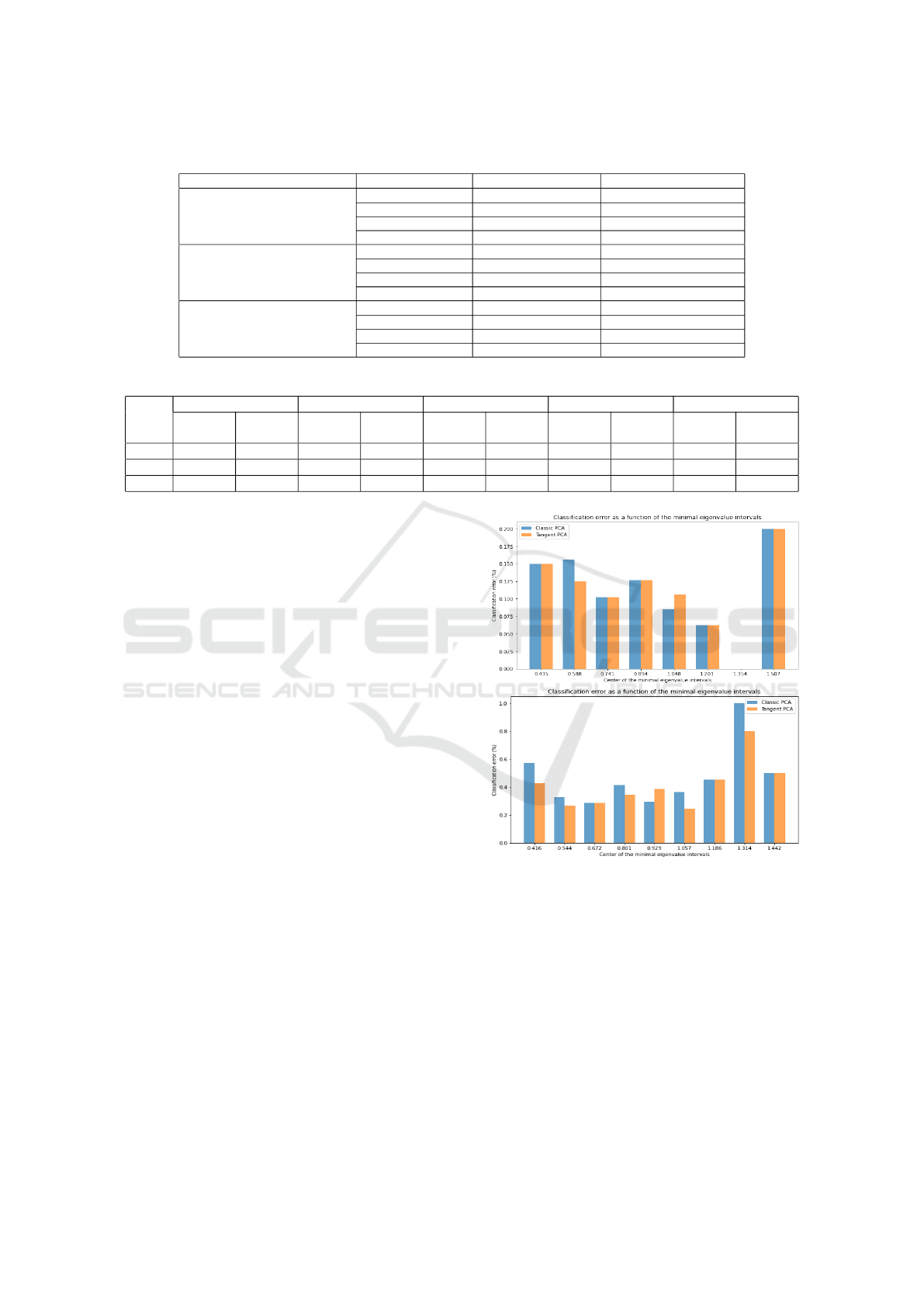
Table 1: Comparison of Method Performance Across Different Cases.

Case Method Mean Accuracy (%) Standard Deviation (σ)

Case 1: Distant Distributions Tangent PCA 100.00 -

Classic PCA 100.00 -

Autoencoder 100.00 -

Harandi’s Method 100.00 -

Case 2: Slightly Interwoven Tangent PCA 88.20 1.09

Classic PCA 88.03 1.56

Autoencoder 89.42 1.67

Harandi’s Method 86.69 1.86

Case 3: Strongly Interwoven Tangent PCA 69.33 1.71

Classic PCA 69.40 1.99

Autoencoder 70.80 1.13

Harandi’s Method 65.67 3.10

Table 2: Performance of Harandi’s Method Across Different Metrics.

Case AIRM Stein Jeffreys Log-Euclidean Euclidean

Mean (%) Std. Dev

(σ)

Mean (%) Std. Dev

(σ)

Mean (%) Std. Dev

(σ)

Mean (%) Std. Dev

(σ)

Mean (%) Std. Dev

(σ)

Case 1 100.00 - 100.00 - 100.00 - 100.00 - 100.00 -

Case 2 86.56 1.47 86.69 1.86 86.66 1.48 86.03 1.60 85.74 1.61

Case 3 65.10 3.42 65.47 2.95 65.49 2.24 65.67 3.10 62.49 3.58

5.3 Classiﬁcation Error According to

the Eigenvalue Range

In this section, we analyze the classiﬁcation error

based on the minimal eigenvalue ranges of the Sym-

metric Positive Deﬁnite (SPD) matrices. The goal is

to explore the relationship between the geometry of

the SPD space, particularly the structure of its convex

cone, and the performance of dimensionality reduc-

tion methods, speciﬁcally classic PCA and tangent

PCA. By segmenting the data into minimal eigenvalue

ranges, we aim to evaluate how these methods per-

form across different regions of the SPD space, par-

ticularly in areas closer to the cone boundaries (where

non-linearity is more pronounced) versus more inter-

nal regions that are almost linear due to the convexity

of the SPD space.

To perform this analysis, we ﬁrst calculate the

minimal eigenvalue of each SPD matrix, which in-

dicates how ”close” a matrix is to the boundary of

the convex cone. Matrices with smaller minimal

eigenvalues are closer to the boundary, where non-

Euclidean curvature is stronger. Conversely, matri-

ces with a larger minimal eigenvalue reside in regions

where the geometry of the space is locally Euclidean.

Then, we report in Figure 3 a histogram including

the classiﬁcation error according to the range of min-

imum eigenvalues for case 2 and case 3.

The classiﬁcation error is generally lower in the

bins corresponding to the largest minimal eigenval-

ues, indicating that classic PCA performs better in re-

gions of the cone where the geometry is almost linear.

This might be explained by the fact that the space SPD

is convex. But, surprisingly, classic PCA slightly out-

Figure 3: Classiﬁcation Errors as a Function of Minimal

Eigenvalues Intervals.

performs tangent PCA in regions with very low mini-

mal eigenvalues. This might be due to the fact that nu-

merical issues may occur when computing the matrix

logarithm of SPD matrices with very small eigenval-

ues. Tangent PCA, on the other hand, outperforms its

classic counterpart for moderately low minimal eigen-

values.

In conclusion, while classic PCA excels in certain

scenarios, tangent PCA’s performance is notably in-

ﬂuenced by the geometric properties of the data. This

study highlights the importance of understanding the

Dimensionality Reduction on the SPD Manifold: A Comparative Study of Linear and Non-Linear Methods

811

underlying structure of data distributions when select-

ing dimensionality reduction techniques, particularly

in complex scenarios where traditional methods may

struggle.

6 CONCLUSION

In this study, we explored various dimensionality re-

duction techniques for Symmetric Positive Deﬁnite

(SPD) matrices, including both linear and non-linear

approaches. The results highlight the lack of robust-

ness of existing methods in handling overlapping dis-

tributions in a classiﬁcation context. Interestingly,

linear and non-linear methods showed similar perfor-

mance with SPD matrices. Two possible explanations

could be: the convexity of the SPD space and the nu-

merical issues raised by the logarithmic calculation.

In future work, a deeper analysis of these methods

according to the local geometry of the SPD space is

needed to discard or validate these hypotheses. In-

vestigating dimensionality reduction in non-convex

spaces is also extremely relevant. Finally, we aim

to extend the dimensionality reduction methods for

SPD matrices to more complex conﬁgurations, such

as highly overlapping distributions.

REFERENCES

Arsigny, V., Fillard, P., Pennec, X., and Ayache, N. (2007).

Geometric means in a novel vector space structure on

symmetric positive-deﬁnite matrices. SIAM Journal

on Matrix Analysis and Applications, 29(1):328–347.

Boumal, N., Mishra, B., Absil, P.-A., and Sepulchre, R.

(2014). Manopt, a Matlab toolbox for optimization on

manifolds. Journal of Machine Learning Research,

15:1455–1459.

Chen, K.-X., Ren, J.-Y., Wu, X.-J., and Kittler, J. (2020).

Covariance descriptors on a gaussian manifold and

their application to image set classiﬁcation. Pattern

Recognition, 107:107463.

Cherian, A., Sra, S., Banerjee, A., and Papanikolopoulos,

N. (2013). Jensen-bregman logdet divergence with ap-

plication to efﬁcient similarity search for covariance

matrices. IEEE Transactions on Pattern Analysis and

Machine Intelligence, 35:2161–2174.

Drira, W., Neji, W., and Ghorbel, F. (2012). Dimension re-

duction by an orthogonal series estimate of the prob-

abilistic dependence measure. In ICPRAM (1), pages

314–317.

Fletcher, P. T. and Joshi, S. (2004). Principal geodesic anal-

ysis on symmetric spaces: Statistics of diffusion ten-

sors. In Sonka, M., Kakadiaris, I. A., and Kybic, J.,

editors, Computer Vision and Mathematical Methods

in Medical and Biomedical Image Analysis, pages 87–

98, Berlin, Heidelberg. Springer Berlin Heidelberg.

Fletcher, P. T., Lu, C., Pizer, S. M., and Joshi, S. C. (2004).

Principal geodesic analysis for the study of nonlin-

ear statistics of shape. IEEE Transactions on Medical

Imaging, 23:995–1005.

echet, M. R. (1948). Les

ements al

eatoires de nature

quelconque dans un espace distanci

Ghorbel, E., Boonaert, J., Boutteau, R., Lecoeuche, S., and

Savatier, X. (2018). An extension of kernel learning

methods using a modiﬁed log-euclidean distance for

fast and accurate skeleton-based human action recog-

nition. Computer Vision and Image Understanding,

175:32–43.

Harandi, M., Salzmann, M., and Hartley, R. (2018). Dimen-

sionality reduction on spd manifolds: The emergence

of geometry-aware methods. IEEE Transactions on

Pattern Analysis and Machine Intelligence, 40(1):48–

62.

Harandi, M. T., Sanderson, C., Hartley, R. I., and Lovell,

B. C. (2012). Sparse coding and dictionary learning

for symmetric positive deﬁnite matrices: A kernel ap-

proach. In European Conference on Computer Vision.

Hinton, G. E. and Salakhutdinov, R. R. (2006). Reducing

the dimensionality of data with neural networks. Sci-

ence, 313(5786):504–507.

Hotelling, H. (1933). Analysis of a complex of statistical

variables into principal components. Journal of Edu-

cational Psychology, 24:498–520.

Jayasumana, S., Hartley, R., Salzmann, M., Li, H., and

Harandi, M. (2015). Kernel methods on riemannian

manifolds with gaussian rbf kernels. IEEE Transac-

tions on Pattern Analysis and Machine Intelligence,

37(12):2464–2477.

Miolane, N., Brigant, A. L., Mathe, J., Hou, B., Guigui, N.,

Thanwerdas, Y., Heyder, S., Peltre, O., Koep, N., Za-

atiti, H., Hajri, H., Cabanes, Y., Gerald, T., Chauchat,

P., Shewmake, C., Kainz, B., Donnat, C., Holmes, S.,

and Pennec, X. (2020). Geomstats: A python package

for riemannian geometry in machine learning.

Pennec, X., Fillard, P., and Ayache, N. (2006). A rieman-

nian framework for tensor computing. International

Journal of Computer Vision, 66(1):41–66.

Tuzel, O., Porikli, F., and Meer, P. (2006). Region covari-

ance: A fast descriptor for detection and classiﬁca-

tion. In Leonardis, A., Bischof, H., and Pinz, A., edi-

tors, Computer Vision – ECCV 2006, pages 589–600,

Berlin, Heidelberg. Springer Berlin Heidelberg.

Tuzel, O., Porikli, F., and Meer, P. (2008). Pedestrian detec-

tion via classiﬁcation on riemannian manifolds. IEEE

Transactions on Pattern Analysis and Machine Intel-

ligence, 30(10):1713–1727.

Vincent, P., Larochelle, H., Bengio, Y., and Manzagol, P.-

A. (2008). Extracting and composing robust features

with denoising autoencoders. In Proceedings of the

25th International Conference on Machine Learning,

ICML ’08, page 1096–1103, New York, NY, USA.

Association for Computing Machinery.

Wang, R., Wu, X.-J., Xu, T., Hu, C., and Kittler, J. (2023).

U-spdnet: An spd manifold learning-based neural

network for visual classiﬁcation. Neural Networks,

161:382–396.

ICAART 2025 - 17th International Conference on Agents and Artiﬁcial Intelligence

812