Ensemble of Neural Networks to Forecast Stock Price by Analysis of

Three Short Timeframes

Ubongabasi Ebong Etim

, Vitaliy Milke

and Cristina Luca

School of Computing and Information Science, Anglia Ruskin University, Cambridge, U.K.

Keywords:

Stock Price Forecasting, Ensemble of Neural Networks, Machine Learning, Futures Analysis, Intraday

Trading, Technical Indicators, Volatility Analysis, Triple Screen Trading System.

Abstract:

Financial markets are known for complexity and volatility, and predicting the direction of price movement of

ﬁnancial instruments is essential for ﬁnancial market participants. This paper aims to use neural networks to

predict the direction of Apple’s share price movement. Historical stock price data on three Intraday timeframes

and technical indicators selected for each timeframe are used to develop and evaluate the performance of

various neural network models, including Multilayer Perceptron and Convolutional Neural Networks. This

research also highlights the importance of selecting appropriate technical indicators for different timeframes

to optimise the performance of the selected neural network models. It showcases the use of neural networks

within an ensemble architecture that tracks the directional movement of Apple Inc. share prices by combining

upward and downward predictions from the three short timeframes. This approach generates a trading system

with buy and sell signals for intraday trading.

1 INTRODUCTION

Historically, price movement predictions have re-

lied on statistical and mathematical methods, includ-

ing but not limited to Relative Strength Index (RSI)

(Singh and Patel, 2021), Fibonacci retracement (Chen

and Zhang, 2022) and moving averages (Gupta and

Sharma, 2023). The use of analysis methods using

technical indicators was widespread until the 2010s,

when advancements in computer power made it pos-

sible to manipulate market participants’ opinion using

false signals on popular technical indicators. Follow-

ing this, neural network based systems for analysing

ﬁnancial markets began to emerge. However, they re-

quire signiﬁcant computer power when analysing raw

transaction data for intraday trading (Lee and Chen,

2023).

Therefore, there is a need for more accurate,

and less labour-intensive methods of predicting price

trends, especially as ﬁnancial markets face large in-

creases in data and transaction volume due to the ad-

vances in telecommunications technology as well as

market institutionalisation (Fabozzi et al., 2013). Ma-

https://orcid.org/0009-0004-0447-4286

https://orcid.org/0000-0001-7283-2867

https://orcid.org/0000-0002-4706-324X

chine learning methods are widely used for their abil-

ity to handle large datasets and non-linearities in data

(Ogulcan E. Orsel, 2022).

This paper focuses speciﬁcally on predicting

the directional movements of prices for Apple Inc.

(AAPL) across multiple Intraday Trading (IT) time-

frames. Each timeframe is characterized by a dif-

ferent intraday trading frequency and employs a dis-

tinct Neural Network (NN) architecture. The goal

is to develop a system that uses combined analyses

from different timeframes to determine the accuracy

of optimal buy or sell decisions on an intraday basis.

This strategy aims to make use of volatility, thus in-

creasing the probability of compounding small prof-

its from minor price changes but many times. The

approach of multiple timeframes is inspired by the

Alexander Elder trading strategy, also known as the

triple-screen trading system. This strategy monitors

three timeframes of the same price trend data, differ-

ing in frequency, using appropriate technical indica-

tors to observe long, medium, and short-term trends

(Elder, 1993), thereby creating a more robust overall

trading strategy. The choice of using AAPL was made

because Apple Inc. is one of the most recognizable

and heavily traded securities on the stock market, pro-

viding an excellent use case for futures price move-

ment forecasting using neural networks. Also, Apple

Etim, U. E., Milke, V. and Luca, C.

Ensemble of Neural Networks to Forecast Stock Price by Analysis of Three Short Timeframes.

DOI: 10.5220/0013183600003890

Paper published under CC license (CC BY-NC-ND 4.0)

In Proceedings of the 17th International Conference on Agents and Artiﬁcial Intelligence (ICAART 2025) - Volume 3, pages 813-820

ISBN: 978-989-758-737-5; ISSN: 2184-433X

813

Inc. has been a publicly traded security for a long

period, hence historical price data spanning several

years is publicly available. The availability of data

makes AAPL ideal for developing and testing neural

network models for predicting price movements. Fi-

nally, the high liquidity and volatility of AAPL shares

represent opportunities for intraday trading, making

it a suitable subject for high-frequency trading strate-

gies. By focusing on AAPL, this study aims to pro-

vide insights that can be generalized to other securi-

ties and commodities in the futures market, thereby

contributing to the broader ﬁeld of ﬁnancial forecast-

ing and trading.

To achieve this aim, the following objectives have

been established:

• Develop and evaluate classiﬁcation models in a

parallel ensemble architecture, utilizing historical

intraday data from the AAPL ticker across three

different timeframes.

• Explore the impact of different technical indica-

tors on the accuracy of the predictions.

• Demonstrate the use of the triple screen trading

philosophy of Dr. Alexander Elder (Elder, 1993)

using new capabilities provided by machine learn-

ing and neural networks.

• Combine the predictions from the parallel ensem-

ble architecture to calculate the ﬁnal accuracy of

the trading system.

The rest of this paper is organised as follows: Sec-

tion 2 investigates the literature and state-of-the-art

studies on the topic; Section 3 describes the dataset,

the technical indicators and the Neural Networks em-

ployed for this research; Section 4 outlines the results;

Section 5 provides discussion about the results and

experiments; ﬁnally the conclusions are drawn in Sec-

tion 6.

2 LITERATURE REVIEW

Traditional methods of ﬁnancial market analysis de-

pend heavily on statistical analysis of historical stock

price data and other variables known as economic or

technical indicators and sentiment indicators (Bollen

et al., 2011). Methods such as time series analy-

sis and the concept of moving averages have reg-

ularly been used in stock price forecasting and are

still widely used for short-term forecasting (Smith

and Williams, 2022). Autoregressive Integrated Mov-

ing Average (ARIMA) models’ level out ﬂuctuations

in pricing to identify trends present in the data (Pa-

tel and Verma, 2024), economic technical indicators

like Relative Strength Index (RSI) present percep-

tions of market movements which include upward

and downward trends (Garcia and Rodriguez, 2022).

The major problem, however, is traditional methods

have difﬁculty in interpreting nonlinear movements,

and this makes them sensitive to market ﬂuctuations

(Lee and Chen, 2023). To this end, the use of ma-

chine learning methods has been employed exten-

sively over the years with the aim of accounting for

such ﬂuctuations and achieving better predictive ac-

curacy(Dhruhi Sheth, 2022). Neural networks are

more effective than Traditional statistical methods in

handling nonlinear ﬁnancial data (Shah and Kumar,

2022).

In (Manickavasagam et al., 2020), the authors ex-

plored hybrid modelling techniques to forecast the

future prices of WTI (West Texas Intermediate) and

Brent crude oil with the primary objective of improv-

ing the accuracy of crude oil price forecasting. The

experiments demonstrated that hybrid models com-

bined with certain model optimization techniques like

IPSO (Improved Particle Swarm Optimisation) and

FPA (Flower Pollination Algorithm) signiﬁcantly im-

prove the accuracy of crude oil price forecasts. The

idea of deriving technical indicators from historical

price data and using them as inputs or features for

training was particularly useful and was adopted for

the purpose of our research.

Forecasting directional movements of stock prices

for intraday trading using Long Short-Term Memory

(LSTM) and Random Forests is presented in (Ghosh

et al., 2022). The authors’ goal was to outperform-

ing traditional market benchmarks by leveraging ad-

vanced machine learning techniques. The experiment

demonstrated that incorporating multiple features, in-

cluding opening prices and intraday returns, into the

ML models improved the prediction accuracy and

trading performance. Both LSTM networks and Ran-

dom Forests were effective in forecasting stock price

movements, with LSTM networks showing a slight

edge in performance. We found the concept of using

historical stock price data for the prediction of direc-

tional movements of stock prices to be valuable for

our research purposes.

Another interesting approach for forecasting stock

index futures intraday returns is presented in (Fu

et al., 2020). The authors have used a functional time

series model in combination with the Block Mov-

ing (BM) technique that provided superior dynamic

forecasting for stock index futures compared to tra-

ditional point prediction methods. This approach bet-

ter captures intraday volatility and market microstruc-

ture, enhancing forecasting accuracy. The paper em-

phasizes the advantages of functional data analysis in

ICAART 2025 - 17th International Conference on Agents and Artiﬁcial Intelligence

814

ﬁnancial forecasting, particularly in high-frequency

trading environments, where traditional methods may

fall short. The dynamic nature of the model allowed

for more accurate and real-time predictions, crucial

for ﬁnancial decision-making.

The potential of neural networks in forecasting

ﬁnancial market volatility is also demonstrated in

(Hamid and Iqbal, 2004). The importance of data

pre-processing, variable selection and proper network

training in achieving accurate predictions are well

highlighted in the paper.

Despite many papers on forecasting ﬁnancial in-

strument prices, there is a signiﬁcant gap in simulta-

neous chronometer analysis of several time-frame sets

using neural networks. Solving this issue is the prin-

cipal scientiﬁc novelty of this paper.

3 METHODS

This section covers various aspects of this research,

including the dataset, the technical indicators used in

each timeframe, the labelling algorithm, and the neu-

ral networks employed.

3.1 Dataset

The dataset for this research consists of Apple Inc

(AAPL) data across the following three intraday time-

frames:

• 5-minute timeframe : 47,350 rows (70% of data)

• 15-minute timeframe: 15,963 rows (24% of data)

• 60-minute timeframe : 3,994 rows (6% of data)

The total number of rows is 68,307 with raw data

features including open, high, low, close and volume.

The data was accessed and downloaded from Alpha

Vantagethrough their API, selected for several rea-

sons, with the primary one being the ease of access

it offers, allowing for straightforward retrieval of data

through API calls.

The technical indicators were extracted from the

raw dataset and used as derived features. In this

research, the following technical indicators are also

included in the input data: momentum, volume,

moving averages, and directional indicators. These

technical indicators are distributed across three time

frames.

Short-Term Timeframe (5 Minutes)

This timeframe is used for analysing charts that focus

on shorter-term movements, typically on an intraday

or very high-frequency basis, such as hourly or every

couple of minutes (Achuthan and Hurst, 2021). The

aim of these charts is largely for determining the most

precise entry and exit points form the trends. Price

action (i.e. logic) is usually tested on the short-term

timeframe for the timing of trades (especially on an

intraday basis). For the purpose of this research, the

technical indicators On-Balance volume, parabolic

stop and reverse (parabolic SAR) and Williams Per-

cent Range (Williams%R) of the closing prices were

chosen for the short-term timeframe.

Medium-Term Timeframe (15 Minutes)

This timeframe is used for analysing charts that are

typically medium-term (i.e. daily charts) (Achuthan

and Hurst, 2021). The aim of these charts is largely

for determining the potential entry points based on

long-term trends seen in the longer term charts. For

the purpose of this research, the technical indicators

Exponential Moving Average, Alligator, Average Di-

rectional Index and Stochastic Oscillator of the clos-

ing prices were chosen for the medium-term time-

frame.

Long-Term Timeframe (60 Minutes)

As the name implies, this timeframe is used for

analysing charts that are typically longer term (i.e.,

weekly or monthly charts). The purpose of these

charts is largely to determine the long-term trends

(Achuthan and Hurst, 2021). For the purpose of

this research, the technical indicators Moving Aver-

age Convergence Divergence, Relative Strength In-

dex, Bollinger Bands and On-Balance-Volume of the

closing prices were chosen for the long-term time

frame.

The choice of these sets of technical indicators for

each of the above timeframes was determined by the

analysis of numerous empirical experiments that are

not of signiﬁcant value to this paper.

3.2 Labelling Algorithm

The labelling algorithm is deﬁned to classify the

movements of closing prices at each time interval

and for each timeframe into three categories: upward

(up), no action (wait) and downward (down) move-

ments. In order to achieve an accurate labelling al-

gorithm for the closing prices of each interval, there

are a number of inputs, with the ﬁrst being the take

proﬁt and stop loss levels denoted as take proﬁt and

stop loss. In addition to these inputs, we include the

Returns, std deviation of asset returns (interpreted

as typical volatility(σ)), the Multiplier (a function

of individual risk appetite) and future returns (the

price change between the current closing price and

the closing price of the immediate future interval).

The multipliers are usually determined by the risk ap-

Ensemble of Neural Networks to Forecast Stock Price by Analysis of Three Short Timeframes

815

petite of the individual investor and are used to arrive

at the take-proﬁt or stop-loss ﬁgure as a multiple of

the volatility.

Equations 1 - 4 are the mathematical interpreta-

tions of the labelling algorithm:

− P

t−1

(1)

where R

is the Return at time t, t is the time of the

current interval, t − 1 is the time at the previous inter-

val, and P is the price of the asset at t.

σ =

N − 1

∑

i=1

−

(2)

where σ denotes the Volatility, R

is the Return at the

current interval,

R is the mean of the returns and N

is the number of returns or the number of intervals

per timeframe. Thus volatility in this context refers to

the degree of variation of trading price from the mean

over time.

= Close

t+1

(3)

is the Future Close Price, t is the time at the cur-

rent interval and t + 1 is the time at the immediate

following interval.

− Close

(4)

where PC

denotes the Price Change at time t, t is the

time at the current interval.

The aim of this labelling approach is to hit as

many take-proﬁt points as possible within the trad-

ing day while minimising the probability of loss. To

achieve this, different multipliers are used for take-

proﬁt and stop-loss points, indicating a higher risk

associated with stop-loss compared to take-proﬁt.A

greater number of take-proﬁt points reﬂects the ob-

jective of maximising proﬁt settlements, whilst fewer

stop-loss points suggest a willingness to take on more

losses but less frequently. Thus:

stoploss = −multiplier ∗ volatility(σ) (5)

and

takepro f it = multiplier ∗ volatility(σ) (6)

For the purpose of this research, stop-loss value

is a magnitude of 2 higher (as a number and not in

value) than take-proﬁt.

Finally, in differentiating the upward and down-

ward signals, we deﬁne certain rules in the code as it

can be seen in the pseudo-code 1

After the labels are created, they are further clas-

siﬁed in two ’attention’ and ’wait’ categories where

while PC

> takepro f it do

signal = UP;

if PC

<= stoploss then

signal = DOWN;

else

Signal = WAIT;

end

Algorithm 1: Labelling Algorithm.

attention consists of the upward and downward sig-

nals. These are then used in the ﬁrst phase of training

and testing as two classes. Figure 1 represents the re-

sults on closing prices after the labelling Algorithm 1

is applied.

Figure 1: Result of Labelling algorithm on closing price as

interval (5 minute interval).

In the second phase of training and testing, only

the attention class from the previous phase is con-

sidered. This class is further split into up and down

classes which are then trained and tested on a set of

three neural networks, each corresponding to a differ-

ent timeframe.

3.3 Neural Network Architecture

The neural network models used in this research in-

clude Multi-Layer Perceptrons (MLP) and Convolu-

tion Neural Networks (CNN). Table 1 shows the neu-

ral networks used in this research and some of their

properties.

Table 1: First and second phase Neural Network character-

istics.

Timeframe Model Num of Features Resampling Method Loss Function

5 min CNN 5 SMOTE Binary cross-entropy

15 min MLP 6 SMOTE Binary cross-entropy

60 min CNN 6 SMOTE Binary cross-entropy

The authors conducted several experiments with

different sets of hyperparameters for each of the neu-

ral network architectures used. The combinations of

hyperparameters that showed the highest results are

described below.

ICAART 2025 - 17th International Conference on Agents and Artiﬁcial Intelligence

816

Multi-Layer Perceptrons (MLP)

The MLP models used are feed-forward neural net-

works consisting of three dense layers with 64 neu-

rons each, and the Rectiﬁed Linear Unit (ReLU) as

the activation function. The Keras API with Tensor-

Flow backend was used for implementation with a bi-

nary cross-entropy loss function. Dropout layers set

20% of the neurons to 0 during training to prevent

overﬁtting. MLP models were used in the 15-minute

timeframe.

Convolutional Neural Networks (CNN)

The CNN’s layers include convolutional, pooling,

ﬂattening, dense and dropout layers as described be-

low.

Convolutional Layers: These layers extract features

from the input data using ﬁlters. The ﬁrst convolu-

tional layer has 64 ﬁlters and a kernel size of 1. Sub-

sequent layers use 128 ﬁlters and apply the ReLU ac-

tivation function for non-linear feature extraction.

Pooling Layers: Two pooling layers with a pool size

of 2 are used to reduce the dimensionality of the fea-

ture maps, allowing the network to focus on the most

signiﬁcant features.

Flatten Layer: Converts the pooled feature maps into

a one-dimensional vector, which is fed into the dense

layers. Dense Layers: These fully connected lay-

ers consist of 64 neurons that use the ReLU acti-

vation function and perform the ﬁnal classiﬁcation

tasks. Dropout Layer: A dropout layer with 50%

dropout is applied to prevent overﬁtting by randomly

disabling half of the neurons during each training it-

eration. Output Layer: The ﬁnal layer uses a sigmoid

activation function for binary classiﬁcation tasks, pro-

ducing a probability for each class.

4 RESULTS

4.1 First Phase Results (Attention &

Wait Signals)

In the ﬁrst phase, each individual model’s ability to

precisely detect Attention and Wait signals is tested.

Since the original dataset after the labelling process

is unbalanced, precision (see equation 7) the primary

metric used for evaluation.

precision =

(T P)

(T P + FP)

(7)

The precision values of each Attention and Wait

classes in the ensemble architecture as well as the

overall precision values for each neural network were

recorded. When Attention values are matched across

all three timeframes, the Attention output from the

ﬁrst stage was accepted. This led to a signiﬁcantly

reduced input for analysis in the second stage, which

no longer contained imbalance, which is more preva-

lent in the Attention and Wait datasets, resulting in a

more realistic outcome (Jin et al., 2022).

Tables 2, 3, 4, and 5 show the results of perfor-

mance metrics from the training (60%) and test(40%)

sets of the Attention (0) and Wait(1) phases, as well as

the overall results for the training and test sets. Figure

2 represents the visualisation of the precision scores

on the test sets.

Table 2: Class performance of models in the Attention and

Wait classiﬁcation training sets.

Class (timeframe) Model Precision % Recall % F-score %

0 Attention (5-min) CNN 72 78 75

1 Wait (5-min) CNN 76 70 73

0 Attention (15-min) MLP 52 55 54

1 Wait (15-min) MLP 52 49 50

0 Attention (60-min) CNN 50 61 55

1 Wait (60-min) CNN 47 37 41

Table 3: Class performance of models in the Attention and

Wait classiﬁcation test sets.

Class (timeframe) Model Precision % Recall % F-score %

0 Attention (5-min) CNN 72 77 74

1 Wait (5-min) CNN 76 70 73

0 Attention (15-min) MLP 57 52 54

1 Wait (15-min) MLP 56 61 59

0 Attention (60-min) CNN 69 58 63

1 Wait (60-min) CNN 64 74 69

Table 4: Overall performance of models in the Attention

and Wait classiﬁcation training sets.

Model (timeframe) Precision % Recall % F-score % Accuracy %

CNN (5-min) 74 74 74 74

MLP (15-min) 52 52 52 52

CNN (60-min) 49 49 48 49

Table 5: Overall performance of models in the Attention

and Wait classiﬁcation test sets.

Model (timeframe) Precision % Recall % F-score % Accuracy %

CNN (5-min) 73 73 73 73

MLP (15-min) 55 54 54 54

CNN (60-min) 66 66 66 66

As it can be seen from Tables 3 and5 and Figure

2, the highest precision of recognition of Attention

and Wait signals is demonstrated on 5-minute and 60-

minute time frames during validation on test sets.

4.2 Second Phase Results (Upward &

Downward Signals)

The training and testing evaluation metric measured

for the NNs in this phase is accuracy (see equation 8).

accuracy =

(T P + T N)

(T P + T N + FP + FN)

(8)

Ensemble of Neural Networks to Forecast Stock Price by Analysis of Three Short Timeframes

817

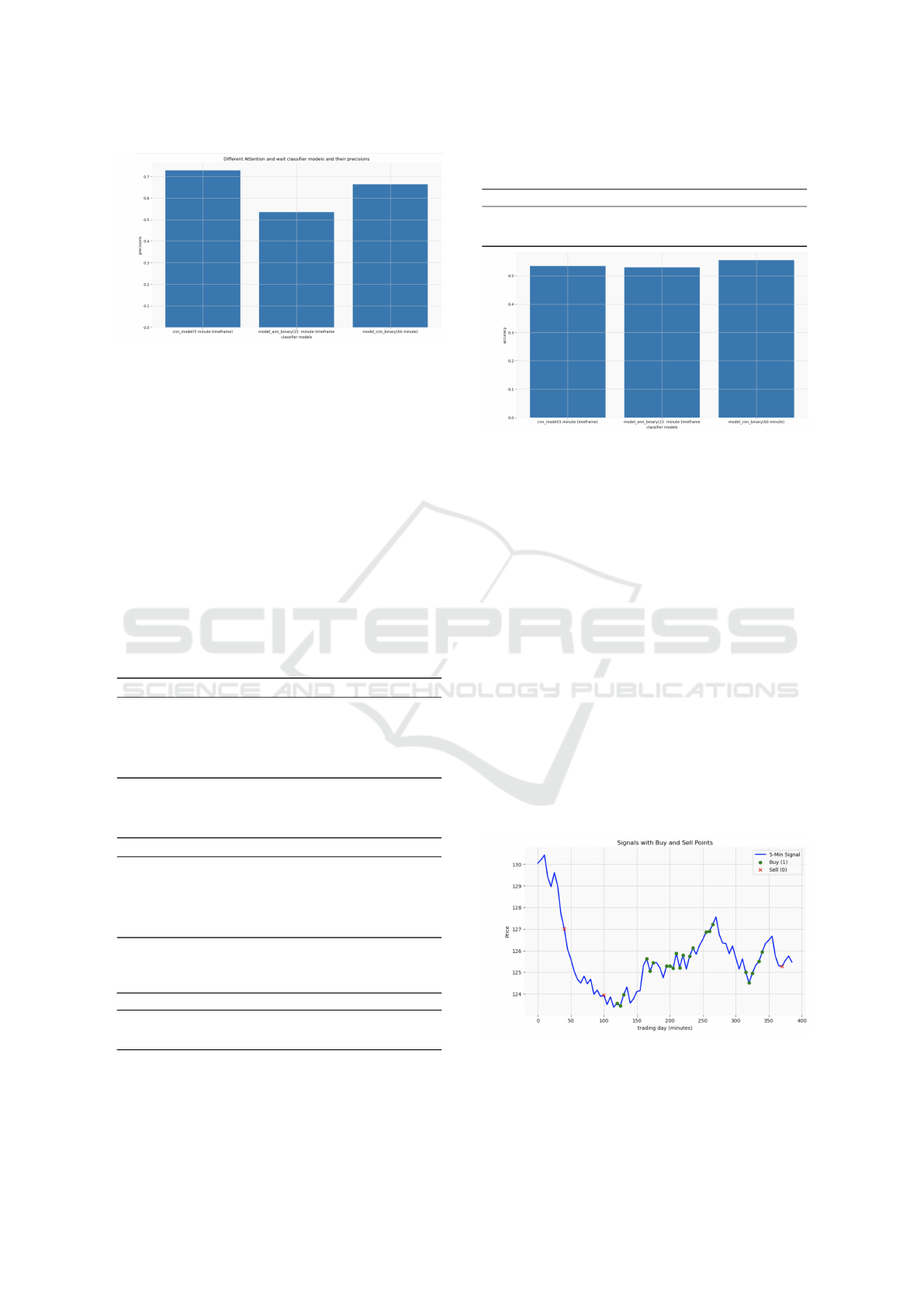
Figure 2: Precision values on Test sets of Attention and Wait

classiﬁcation NNs.

The accuracy values of each Up and Down class in

the ensemble architecture of the second phase, as well

as the precision and recall values for each neural net-

work were recorded. Macro average values were se-

lected for the overall values recorded, as they account

equally for each class in the classiﬁcation task. This

approach is appropriate since the imbalance in the Up

and Down datasets is far lower than in the Attention

and Wait datasets. (Jin et al., 2022). Tables 6, 7,

8, and 9 represent the results of performance metrics

achieved for the training(60%) and test(40%) sets of

the Up(0) and Down(1) phase as well as the overall

results for the training and test sets.

Table 6: Class performance of models in the Up and Down

classiﬁcation training sets.

Class (timeframe) Model Precision % Recall % F-score %

1 Up (5-min) CNN 61 50 55

0 Down (5-min) CNN 59 70 64

1 Up (15-min) MLP 56 61 59

0 Down (15-min) MLP 58 53 56

1 Up (60-min) CNN 64 68 66

0 Down (60-min) CNN 68 64 66

Table 7: Class performance of models in the Up and Down

classiﬁcation test sets.

Class (timeframe) Model Precision % Recall % F-score %

1 Up (5-min) CNN 60 43 50

0 Down (5-min) CNN 53 70 61

1 Up (15-min) MLP 56 61 59

0 Down (15-min) MLP 57 52 54

1 Up (60-min) CNN 64 61 62

0 Down (60-min) CNN 62 61 62

Table 8: Overall performance of models in the Up and

Down classiﬁcation training sets.

Model (timeframe) Accuracy % Recall % F-score % Precision %

CNN (5-min) 60 60 60 60

MLP (15-min) 52 52 52 52

CNN (60-min) 66 66 66 66

Figure 3 represents the visualisation of the accu-

racy metric on the test sets for each timeframe in the

second (Up & Down) phase.

Table 9: Overall performance of models in the Up and

Down classiﬁcation test sets.

Model (timeframe) Accuracy % Recall % F-score % Precision %

CNN (5-min) 53 56 56 57

MLP (15-min) 52 57 56 57

CNN (60-min) 56 63 63 63

Figure 3: Visualization of the accuracy values for test sets

of Up and Down classiﬁcation neural networks.

As seen from the Tables 7, 9 and Figure 3, the

overall accuracy on test sets is reduced; however,

combining the predictions using ensemble of the

triple timeframe increases ﬁnal accuracy signiﬁcantly.

4.3 Final Phase Results (Overall

Upward & Downward Prediction)

Finally, the total accuracy of the triple timeframe sys-

tem (5-min, 15-min and 60-min) is calculated by syn-

chronising the predictions in each timeframe and di-

viding the ﬁnal number of upward signals by the total

number of signals on a given trading day, and convert-

ing the answer to a percentage. Upward signals on a

given trading day are correct responses, considering

the predictions of the triple timeframe system up dur-

ing this day. Figure 4 represents the visualisation of

the ﬁnal up and down data points from which ﬁnal

accuracy is determined.

Figure 4: Visualisation of buy and sell signals for 1st trading

day.

Figure 4 show a total of 25 (22 Buy (green dots)

and 3 Sell (red crosses)) signals for the given trading

ICAART 2025 - 17th International Conference on Agents and Artiﬁcial Intelligence

818

day. The accuracy of the system on this trading day is

88%, as calculated in equation 9.

Accuracy =

∗ 100 = 88% (9)

Using a single time frame as input usually demon-

strates lower levels of accuracy; for example, 61% ac-

curacy was shown in (Qin, 2024) to predict the AAPL

stock trend.

5 DISCUSSION

This section outlines the rationale behind key deci-

sions made regarding the overall research direction.

It covers several aspects including the use of tech-

nical indicators, historical stock price data for deriv-

ing technical indicators and the multiple timeframe

ensemble architecture which was modelled after the

triple screen trading strategy of Dr. Alexander Elder

(Elder, 1993).

5.1 Triple Timeframe Predictive

Ensemble Model

Technical indicators are used in addition to price data

in training different neural networks across three dif-

ferent timeframes and two phases of training. The

ﬁrst phase classiﬁes signals into classes suggesting

action (Attention) and inaction (Wait), whilst the sec-

ond phase focuses on classifying the attention signals

into two classes predicting upward or downward price

movement. This approach is novel, as although pre-

vious studies have employed the triple screen trading

strategy of (Elder, 1993), which inspired the use of

three timeframes, the combination of multiple train-

ing phases for different speciﬁc purposes and the use

of technical indicators as features, has not been ex-

plored. Additionally, it is worth mentioning that the

signals, which were used for the labelling of the up-

ward and downward movement of the prices, were en-

tirely derived from the closing price volatility, mak-

ing another unique aspect of this research. Typically,

volatility is determined using concepts such as bid-

ask spread (Milke, 2023), Average True Range (ATR)

and True Range (TR) (Team, 2022).

5.2 Final Accuracy

The approach explored in this research involves

analysing the predictions made by each neural net-

work model across different timeframes in a time-

synchronised manner. Following this, a decision is

made by determining whether the predictions at each

time step in each timeframe coincide with those on

the other two timeframes. If the answer is yes, then

the uniformity suggests a ’Buy’ signal (ﬁnal ”1”) or a

‘Sell’ signal (ﬁnal ”0”). If the answer is no, the lack of

uniformity across the timeframes indicates inaction.

Thus, the ﬁnal accuracy is calculated by dividing the

number of ‘buy’ signals by the total number of signals

and the result is the probability of accuracy.

This ensemble approach to making a ﬁnal deci-

sion allows for an increase in the forecast accuracy

of the direction of the future movement of the stock

and, therefore, reduces the risk of an incorrect deci-

sion. Focusing on many small proﬁts accelerates the

capital increase, just as small daily interest payments

increase capital many times over due to the compound

interest formula.

6 CONCLUSIONS

This paper explores the use of neural networks to pre-

dict the directional movement of stock prices on intra-

day trading using an Apple Inc. case study. The pa-

per describes the integration of multiple timeframes

of intraday data, using technical indicators as features

for several neural networks, such as CNN and MLP,

within an ensemble architecture. The use of stock

price data to predict the directional movement of fu-

tures introduces some limitations, as futures market

data have distinct properties that are not captured in

stock price data. As such, further reﬁnements are

needed, in line with future work, to optimize perfor-

mance for practical trading applications. Overall, this

paper offers novel ﬁndings into the use of neural net-

works for ﬁnancial forecasting in intraday trading.

A potential future direction for this research is

scalability across other securities and using a more

robust measure of volatility, such as Average True

Range (ATR) or True Range (TR) in order to account

for the full range of price volatility. The exploring of

price movement patterns can be done with Japanese

candlesticks (Milke, 2023). This approach cold be

also applied to futures contracts as well as other ﬁ-

nancial instruments other than stocks, thus account-

ing for the difference in structure of futures data and

other ﬁnancial instruments.

REFERENCES

Achuthan, S. and Hurst, B. (2021). The Ultimate Guide to

Trading with Multiple Time Frames. Wiley, Hoboken,

NJ. Accessed August 7th, 2024.

Bollen, J., Mao, H., and Zeng, X.-J. (2011). Twitter mood

Ensemble of Neural Networks to Forecast Stock Price by Analysis of Three Short Timeframes

819

predicts the stock market. Journal of Computational

Science, 2(1):1–8.

Chen, Y. and Zhang, M. (2022). Evaluating the predictive

power of ﬁbonacci retracement in stock market fore-

casting. International Journal of Financial Studies,

13:22–38. [Online; accessed 3rd-September-2024].

Dhruhi Sheth, M. S. (2022). Predicting stock market us-

ing machine learning: best and accurate way to know

future stock prices. International Journal of System

Assurance Engineering and Management. Available

at: https://link.springer.com/article/10.1007/s13198-0

21-01357-x.

Elder, A. (1993). Trading for a Living: Psychology, Trad-

ing Tactics, Money Management. John Wiley & Sons.

[Online; accessed 3rd-September-2024].

Fabozzi, F. J., Modigliani, F., Jones, F. J., and Ferri, M. G.

(2013). Foundations of Financial Markets and Insti-

tutions. Prentice Hall, Upper Saddle River, NJ, 4h

edition.

Fu, Y., Su, Z., Xu, B., and Zhou, Y. (2020). Forecasting

stock index futures intraday returns: Functional time

series model. Journal of Advanced Computational In-

telligence and Intelligent Informatics, 24(3):265–271.

Accessed August 4th, 2024.

Garcia, L. and Rodriguez, E. (2022). Evaluating the ef-

fectiveness of technical indicators in ﬁnancial mar-

kets: A nonlinear perspective. Quantitative Finance

and Economics, 5:122–138. [Online; accessed 3rd-

September-2024].

Ghosh, P., Neufeld, A., and Sahoo, J. K. (2022). Forecast-

ing directional movements of stock prices for intra-

day trading using lstm and random forests. Finance

Research Letters, 46:102280. Accessed August 4th,

2024.

Gupta, R. and Sharma, P. (2023). The role of moving av-

erages in predicting stock price movements: A statis-

tical perspective. Statistical Finance Journal, 58:78–

91. [Online; accessed 3rd-September-2024].

Hamid, S. A. and Iqbal, Z. (2004). Using neural networks

for forecasting volatility of s&p 500 index futures

prices. Journal of Business Research, 57(10):1116–

1125. Selected Papers from the third Retail Seminar

of the SMA.

Jin, X., Liu, Q., and Sun, W. (2022). Imbalanced class dis-

tribution and performance evaluation metrics: A sys-

tematic review of prediction accuracy for determining

model performance in healthcare systems. PLOS Dig-

ital Health, 1(2).

Lee, M. and Chen, D. (2023). Challenges in predicting

stock market movements using traditional statistical

methods. Financial Econometrics Review, 18:88–102.

[Online; accessed 3rd-September-2024].

Manickavasagam, J., Visalakshmi, S., and Apergis, N.

(2020). A novel hybrid approach to forecast crude

oil futures using intraday data. Technological Fore-

casting and Social Change, 158:120126. Accessed

August 4th, 2024.

Milke, V. (2023). Intraday machine learning for the secu-

rities market. Phd thesis, Anglia Ruskin University.

[Online; accessed 2nd-September-2024].

Ogulcan E. Orsel, S. S. Y. (2022). Comparative study of

machine learning models for stock price prediction.

arXiv preprint arXiv:2202.03156. accessed on 5th

Septembr 2024.

Patel, R. and Verma, A. (2024). Application of arima

models in ﬁnancial market forecasting: An empirical

study. International Journal of Forecasting, 40:65–79.

[Online; accessed 3rd-September-2024].

Qin, W. (2024). Predictive analysis of aapl stock trend by

random forest and k-nn classiﬁer. Highlights in Busi-

ness, Economics and Management, 24:1418–1422.

Shah, P. and Kumar, R. (2022). A comprehensive review

on neural network-based approaches in ﬁnancial fore-

casting. Journal of Financial Data Science, 4:123–

145.

Singh, A. and Patel, V. (2021). Price prediction using tech-

nical indicators: A comparative study. Journal of Fi-

nancial Markets, 45:101–115. [Online; accessed 3rd-

September-2024].

Smith, J. and Williams, S. (2022). A review of time series

forecasting techniques in ﬁnancial markets. Journal

of Financial Analysis, 59:102–118. [Online; accessed

3rd-September-2024].

Team, Q. (2022). What is atr? average true range as a

volatility indicator. https://quantstrategy.io/blog/what

-is-atr-average-true-range-as-a-volatility-indicator/.

Accessed: 2024-09-05.

ICAART 2025 - 17th International Conference on Agents and Artiﬁcial Intelligence

820