Learning to Run a Marathon: Avoid Overﬁtting to Speed

Kriszti

an G

abrisch

and Istv

an Megyeri

University of Szeged, Dugonics Square 13, Szeged, 6720, Hungary

Keywords:

Reinforcement Learning, Robustness, Humanoid, Walker2D, Hopper.

Abstract:

Research and development in reinforcement learning is a dynamically evolving ﬁeld, with a particular focus

on robustness and continuous optimization of reward. The models learned in the OpenAI GYM and Mujoco

environments investigated here seek to make different dummies move in one direction as fast as possible

without losing stability. During the learning process, the models are usually trained for a predeﬁned number

of steps, which can act as a limiting factor and result in an unexpected limitation in the model performance.

This iteration limitation can contribute to model instability, often leading to model failure, thus hindering

the model’s ability to collect additional rewards. In our observations, we also note that models face a major

problem in simultaneously optimizing their stability and speed. We traced the learning process of the models

through twenty checkpoints, and deﬁned various metrics to select the models that are most suitable for us.

We have noticed that the model obtained at the last checkpoint does not always perform the best, so it is

worth monitoring the learning process so we can get better models during the learning process. Our code and

pretrained models are available at https://github.com/szegedai/rl run marathon.

1 INTRODUCTION

Reinforcement Learning (RL) has seen signiﬁcant ad-

vances in recent years, marked by impressive suc-

cesses in various domains. Applications such as

mastering complex games (e.g., AlphaGo and Ope-

nAI’s Dota 2 agents) and autonomous robotics control

demonstrate RL’s potential to handle highly dynamic

and complex environments effectively. These devel-

opments have been driven in part by the emergence

of deep learning-based algorithms that offer improved

learning efﬁciency and performance, such as Trust

Region Policy Optimization(TRPO) (Schulman et al.,

2017a), Proximal Policy Optimization (PPO) (Schul-

man et al., 2017b) and Smoothed Proximal Policy

Optimization (SPPO) (Sun et al., 2024). These al-

gorithms seek to strike a balance between exploration

and exploitation, offering better policy updates within

the constraints of non-linear approximators like neu-

ral networks.

While TRPO and PPO have improved sample ef-

ﬁciency and stability compared to earlier methods,

their complexity presents challenges. For example,

TRPO requires complex second-order derivatives,

making it computationally expensive. PPO improves

https://orcid.org/0009-0005-3909-2218

https://orcid.org/0000-0002-7918-6295

upon this by simplifying the optimization process

while ensuring stability. Despite these advancements,

further reﬁnements are needed, especially when con-

fronted with adversarial environments.

Recently, research has shifted focus to adver-

sarial robustness in RL. Adversarial training meth-

ods, such as stochastic gradient Langevin dynam-

ics (SGLD) (Sun et al., 2024) and adversarially-

augmented PPO (SAPPO) (Zhang et al., 2020) and

Worst-Case-Aware PPO (WocaR-PPO) (Liang et al.,

2022), seek to mitigate vulnerabilities to adversar-

ial perturbations. These methods focus on enhanc-

ing model stability and robustness against adversarial

examples, which can dramatically affect the perfor-

mance of RL policies in real-world settings.

In this study, we address a speciﬁc shortcoming in

the current training processes of RL policies. Many

policies tend to overﬁt speed during training, which

leads to higher rewards. However, this often results in

degraded model stability towards the end of the train-

ing phase. Here, we deﬁned stability as the distance

taken by an agent before a fall and observed a mis-

match between speed and stability during the train-

ing. To overcome this problem, we propose a novel

model selection approach that takes into account mul-

tiple metrics, such as speed, distance taken to fall, and

time taken to fall, and ensures a more balanced model

selection.

Gábrisch, K. and Megyeri, I.

Learning to Run a Marathon: Avoid Overﬁtting to Speed.

DOI: 10.5220/0013186200003890

Paper published under CC license (CC BY-NC-ND 4.0)

In Proceedings of the 17th International Conference on Agents and Artiﬁcial Intelligence (ICAART 2025) - Volume 3, pages 829-836

ISBN: 978-989-758-737-5; ISSN: 2184-433X

829

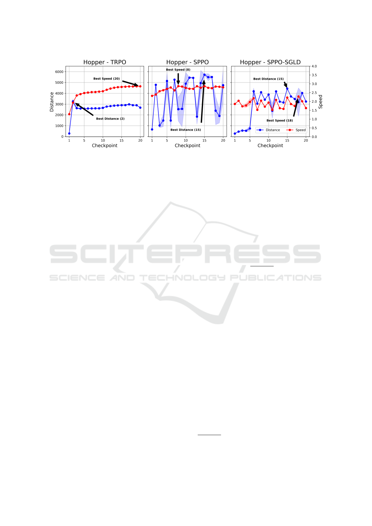
Figure 1: Distance to fall and speed is displayed as the function of hopper model checkpoints for TRPO,SPPO and SPPO-

SGLD algorithm. The checkpoints are evaluated using 100 seeds and average score and standard deviation are displayed.

There is a noticeable mismatch between the two metrics for all the algorithms. The model tends to optimize only speed and

distance can be unstable during training.

Furthermore, we advocate increasing the environ-

ment step limit during training to strengthen the mod-

els and improve long-term performance. This point

is typically unexplored and set to a predeﬁned ﬁxed

number. By extending the training horizon and us-

ing more robust evaluation metrics, we attempt to en-

hance the stability of RL models, ensuring that they

remain effective even in more complex and adversar-

ial environments.

Here, we describe the overﬁtting to speed for three

algorithms TRPO, SPPO, and SPPO-SGLD, which is

also shown by the learning curve of the Hopper en-

vironment in Fig. 1. Then, we demonstrate improved

stability via a novel data collection using dynamic en-

vironment step limits to simulate longer runs, while

adjusting the number of episodes and the batch size at

the same time so the compute, memory requirement,

and running time remain the same. We also applied

our new data collection technique on the SPPO algo-

rithms, but in this case it did not yield any improve-

ment, however with a good model choice, for which

we used three different metrics, we can obtain a model

with a more robust performance than that got at the

last state of the training.

2 POLICY OPTIMIZATION

In this section, we review the TRPO and SPPO al-

gorithms that we shall use as baselines in our exper-

iments. Then, we describe the proposed heuristics

used to modify episode number and environment step

limit during training.

2.1 Baseline Methods

Trust Region Policy Optimization (TRPO) is a policy

optimization algorithm used in reinforcement learn-

ing (RL). It seeks to improve the stability and per-

formance of policy updates by ensuring that the new

policy stays within a ”trust region” of the old policy,

hence avoiding large, destabilizing policy updates.

TRPO optimizes the policy by solving the follow-

ing constrained optimization problem:

max

s∼π

old



(a|s)

old

(a|s)

old

(s,a)



(1)

s∼π

old





old

(a|s)∥π

(a|s)



≤ δ (2)

Here, θ represents the policy parameters, π

(a|s) is

the probability of taking action a in state s under pol-

icy π

, and A

old

(s,a) is the advantage function. The

KL divergence term ensures that the new policy does

not deviate signiﬁcantly from the old policy by re-

stricting the change in policy within a small step δ.

TRPO’s constraint-based approach provides that

policy changes are smooth, making it more reliable

for tasks where large policy updates might lead to per-

formance collapse. The algorithm is often applied in

continuous action spaces and high-dimensional prob-

lems. However, the constrained problem requires us-

ing second-order methods and this might be unsuit-

able for deep neural networks. A more practical so-

lution is to transform the constraint into the objective

via a penalization term. The new penalized TRPO ob-

jective is shown in Eq. (3).

max

s∼π

old



(a|s)

old

(a|s)

old

(s,a) −βKL



old

(a|s)∥π

(a|s)





(3)

ICAART 2025 - 17th International Conference on Agents and Artiﬁcial Intelligence

830

Table 1: Major hyperparameters are shown for SPPO and TRPO algorithms an the three training methods. Note, the batch

size, episodes and max iteration changes in a way that the amount of data seen by the three training methods are comparable.

Algorithm ENV Hyper parameter

Training methods

Baseline Static Dynamic

TRPO All Env Batch Size(episode) 20 20/10 160/80/40/20/10/5

Hopper Training length 30 ×10

ep 15/7.4 ×10

ep 21.8 ×10

Env Max Iter 10

1/2 ×10

125/.../4000

Update Steps 1.5 ×10

Walker2d

Training length 25.2 ×10

ep 12.4/6 ×10

ep 21.3 ×10

Env Max Iter 10

1/2 ×10

125/.../4000

Update Steps 1.26 ×10

Humanoid

Training length 20 ×10

ep 10/5 ×10

ep 150 ×10

Env Max Iter 10

1/2 ×10

125/.../4000

Update Steps 10

SPPO Hopper

Batch Size(iteration) 2048 - 2048

Episodes 0.96 ×10

ep - 0.96 ×10

Env Max Iter 10

- 20 ×10

Update Steps 0.96 ×10

β is a hyperparameter that controls the

strength of the KL divergence penalty. The term



old

(a|s)∥π

(a|s)



ensures that large updates

to the policy (large KL divergence) are penalized,

encouraging smoother updates similar to the original

TRPO’s constraint.

In this penalized version, instead of using a hard

constraint on the KL divergence, we penalize devia-

tions directly in the objective function by scaling the

KL divergence term with β. This makes the optimiza-

tion process simpler and allows us to balance between

policy improvement and policy stability.

Proximal Policy Optimization (PPO) is a simpli-

ﬁed alternative to TRPO that improves efﬁciency by

removing the need to solve a constrained optimiza-

tion problem. Instead, PPO uses a clipped surrogate

objective to limit the change in policy at each update,

effectively mimicking the trust region concept with-

out complex computations.

The PPO objective is deﬁned as follows:

max

s∼π

old

[min



r(θ)A

old

(s,a),

clip(r(θ), 1 −ε, 1 + ε)A

old

(s,a)



] (4)

where r(θ) =

(a|s)

old

(a|s)

is the probability ratio between

the new and old policies, and ε is a hyperparameter

that controls the clipping range. The clipped term

ensures that the update does not excessively shift the

policy, avoiding large jumps.

PPO simpliﬁes the optimization process and re-

duces computational overhead while yielding a simi-

lar performance to TRPO. It is widely used in various

RL applications due to its balance of simplicity and

effectiveness.

2.2 Modify Episode Number and

Environment Limit During Training

In the baseline methods, a ﬁxed environment limit and

a ﬁxed number of episodes are collected for model

updates. This way, we can have a suitably controlled

amount of training samples and budget compute with

a simple implementation. However, for robust and

stable models we shall deﬁne a more appropriate data

collection method. We shall deﬁne two simple heuris-

tics, to test our hypotheses which can collect the same

amount of data as our baseline methods so that they

have a comparable compute cost.

Static. The static models were run with the baseline

settings until half of the training, then in the subse-

quent phase we halved the batch size and doubled the

iteration limit, and in the second phase of training,

we trained until we had nearly half of the remaining

episode numbers, all to guarantee that the required re-

sources did not deviate from the baseline models. We

hiphotetize that the model trained in the longer run but

with fewer episodes can achieve similar speed and is

more stable.

Dynamic. The dynamic models started their learning

process with an iteration limit of 125 and a batch size

of 160. As 2/3 of the episodes in a batch reached its it-

eration limit, we halved the batch size and doubled the

iteration limit. By doing this with the same resource

requirements, we were able to show that our model

runs longer and dynamically increases the problem

complexity as the model improves. The list of the

batch sizes used and iteration limits are given in Ta-

ble 2.

Learning to Run a Marathon: Avoid Overﬁtting to Speed

831

Table 2: Dynamic models episode and iteration number

scaling. When the iteration limit has been reached in 2/3

of the given number of episodes, we move to the next state,

thus increasing the iteration limit during the learning pro-

cess.

State ID Batch Size Iteration

1 160 125

2 80 250

3 40 500

4 20 1000

5 10 2000

6 5 4000

SPPO-dynamic The baseline models were trained

over 960 episodes on a 1000 iteration bound and up-

dated every 2048 iterations. By comparison, the dy-

namic models changed to the extent that they were

allowed a total of 20,000 iterations on the environ-

ment, provided there were no loss in stability before

we reset the environment. Since the algorithm up-

dates the model every 2048 iterations, we did not need

to change any other parameters values.

The three training methods and the corresponding

hyperparameters are shown in Table 1 for each given

environment. The hyperparameters controlling data

collection were selected in a way so that the GPU,

CPU, memory, and time requirements did not change

during training compared to the baseline. However,

the evaluations need for model selection take signif-

icantly more time. For example, SPPO models eval-

uations were conducted across 100 seeds, each with

a 2000-iteration limit. In contrast, training runs for 2

million iterations and includes backward passes, ef-

fectively doubling the computational load compared

to evaluations, which involve only forward passes.

3 ROBOTIC CONTROL

ENVIRONMENTS

We shall look at three environments, which are de-

scribed in this section. The selected models had to

easily fall so stability could be easily measured and

the model do not get stuck in a state where it was not

moving anywhere, but just trying to avoid falling. For

example, in the Ant environment, the model was stuck

and couldn’t move because of its four legs. To have a

more representative evaluation, we selected the envi-

ronments to represent different levels of complexity.

Out of the environments listed here, in terms of

complexity, the Humanoid environment is the most

complex, with a high-dimensional action space and

an extremely large observation space, requiring ad-

vanced policies for control and balance. The Hop-

per is the simplest, featuring a low-dimensional ac-

tion space and a small observation space, making it

suitable for basic control tasks. The Walker2d falls

in between, with moderate complexity due to action

space and observation space, balancing controllabil-

ity and challenge.

3.1 Hopper

The environment described is based on (Durrant-

Whyte et al., 2012). The study focuses on increas-

ing the number of independent state and control vari-

ables compared to traditional control environments.

The model represents a two-dimensional hopper with

a single leg, composed of four main body parts: the

torso, thigh, leg, and foot. The objective is to perform

forward-moving hops by applying torques to the three

hinges that connect these body parts.

The action space has three dimensions and is con-

tinuous in the range of [−1, 1] where the three values

represent the torques applied at the hinges. Obser-

vations consist of the positional values of the hop-

per’s body parts, followed by the velocities of these

parts. The entire observation is a vector of an 11-

dimensional space with positions ordered before ve-

locities.

3.2 Walker2D

This environment is an extension of the hopper envi-

ronment (Durrant-Whyte et al., 2012). Here, a two-

legged robot is introduced, allowing it to walk for-

ward instead of hop. Similar to other Mujoco envi-

ronments, it aims to increase the number of indepen-

dent state and control variables compared to classic

control setups.

The walker is a two-dimensional ﬁgure with a sin-

gle torso at the top, two thighs, two legs, and two feet.

The task is to coordinate the legs and feet to move for-

ward by applying torques to the six hinge joints con-

necting the body parts. The action space is continuous

and has a range of [−1,1] with six values representing

torques. Observations include positional values of the

body parts followed by their velocities, organized into

a vector of a 17-dimensional space.

3.3 Humanoid

The humanoid enviroment (Tassa et al., 2012) fea-

tures a 3D bipedal robot designed to simulate human

motion. The robot has a torso with two arms and two

legs, where the arms and legs are composed of two

links each, representing the knees and elbows. The

ICAART 2025 - 17th International Conference on Agents and Artiﬁcial Intelligence

832

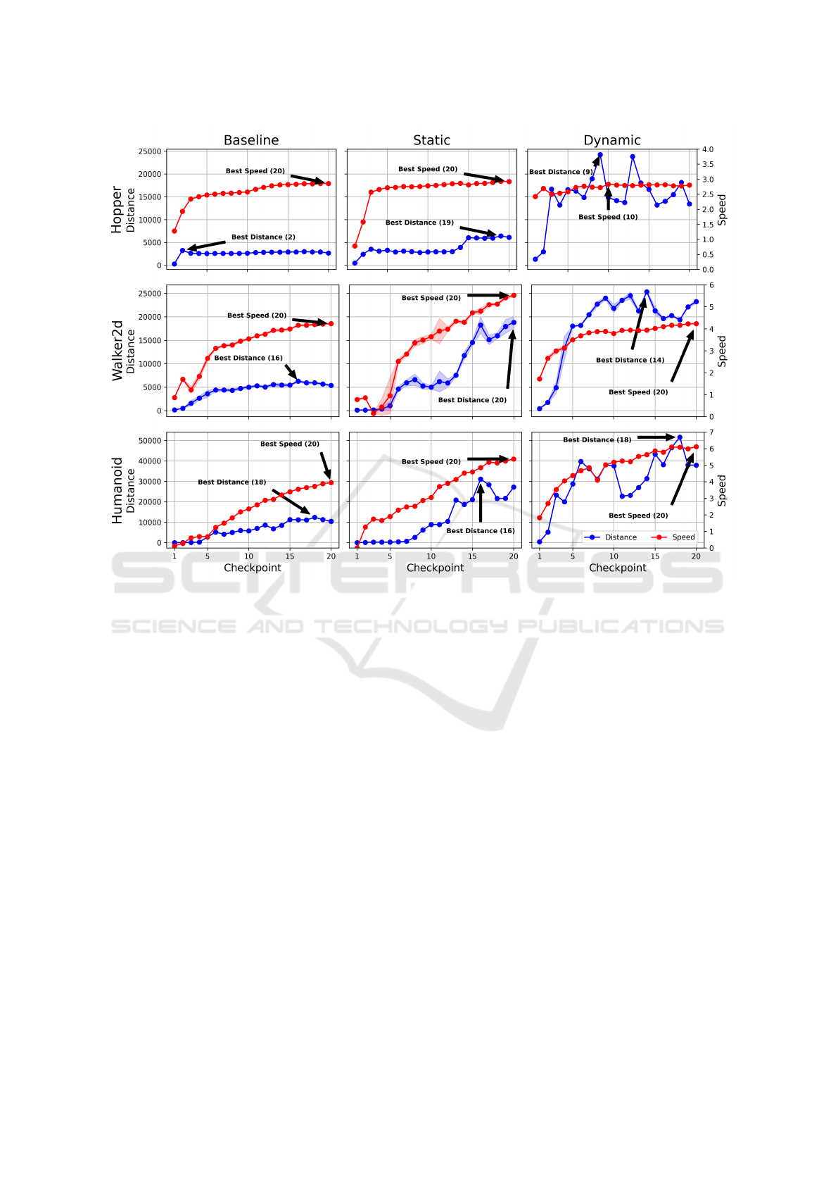
Figure 2: Hopper, Walker2D, and Humanoid checkpoints are displayed for all three training algorithms as distance vs speed.

Static and dynamic models are able to run a longer distances, in some cases speed is also improved.

objective is to walk forward as quickly as possible

without falling.

The action space is continuous and has a range of

[−1,1] with 17 values representing the torques ap-

plied to the robot’s hinge joints. Observations in-

clude positional data for various body parts, followed

by their velocities, organized into a 376-dimensional

vector.

3.4 MuJoCo

We used the 2.1.0 MuJoCo (Todorov et al., 2012)

version and python 3.8, using the robotics models

provided by OpenAI GYM, which deﬁned the com-

plete environment and its basic functions, including

our stopping condition, reward function and observa-

tion space after each step. The reward function calcu-

lates the velocity based on the past and current posi-

tion on the x coordinate, scales this by a constant and

ﬁnally adds a healthy reward, which is a ﬁxed value,

to reward the stability of the model.

The environments are physics-based simulations

set on ﬂat terrains. We use the MuJoCo engine to

model realistic dynamics, including friction, gravity,

and collisions, enabling accurate simulation of rigid

bodies and joints. These environments are designed

for continuous control tasks, ideal for testing rein-

forcement learning algorithms in simulated physical

systems.

4 EXPERIMENTAL SETUP

In this section, we describe our training parameters

for the TRPO and SPPO algorithms. Then, we de-

scribe the process of checkpoints saving policy evalu-

ation and the used metrics to quantify the model per-

formances.

4.1 TRPO Training Hyper Parameters

The TRPO training and evaluation is based on the

repository from https://github.com/pat-coady/trpo.

During the training process, two neural networks

were optimized: policy and value function. The algo-

rithm was applied to the Hopper, Walker2d and Hu-

manoid environments.

Learning to Run a Marathon: Avoid Overﬁtting to Speed

833

The networks learning the policy and value func-

tion use random normal initializer and tanh activation

function. Each network has two hidden layers.

As policy’s training objective, we used Eq. (3)

augmented with a Hinge loss. In the two hidden layers

of the policy network, there are int(

√

∗10 ∗d

∗10)

and d

×10 neurons respectively, where d

and d

re-

fer to the dimensions of the observation and action

space.

For the value function network, the hidden lay-

ers have int(sqrt(d

×10 ×5)) and 5 neurons respec-

tively. We used a squared loss function and Adam

(Kingma and Ba, 2017) as optimizer. We also use

a replay buffer, which consists of the data collected

in the previous learning step. We concatenate this

with the training data, shufﬂe the data, and update the

model with it.

The learning rate heuristic was computed based on

the size of the neural network, which was tuned on the

Hopper-v1 environment:

9×10

−4

(int(

√

×10)∗(d

×10)))

. We

used a dynamic learning rate schedule during train-

ing based on the optimized loss values. We also use a

discount factor of 0.995 to help us ﬁnd new and possi-

bly better steps and maximise the longer-term reward

function. We use λ = 0.98 for Generalized Advantage

Estimation (GAE)(Schulman et al., 2016). For policy

update, we also use a kl

targ

= 0.003 value as the D KL

target in the loss function.

4.2 SPPO Training Hyper Parameters

The SPPO vanilla and SPPO-SGLD (Sun et al.,

2024) training and evaluation is based on the

repository from https://github.com/Trustworthy-ML-

Lab/Robust HighUtil Smoothed DRL.

We use the orthogonal initialization scheme from

OpenAI to initialize policy weights and use the tanh

activation function. As the optimizer, we use adam

with a 4 × 10

−4

learning rate initially and a linear

learning rate annealing. For loss calculation, we use

GAE-based loss for the value function. The network

has one hidden layer with size 64 neurons.

For the value function, we use the orthogonal ini-

tialization scheme from OpenAI to initialize weights

and use tanh activation function. For loss calculation,

we use a GAE-based loss. We use the adam optimizer

with a 3 ×10

−4

learning rate initially. Value function

has one hidden layer with size 64.

4.3 Checkpoint Saving

We aim to analyze the policy stability during the train-

ing process so we save 20 checkpoints from each

model training. For the TRPO baseline models at ev-

ery 1500th episode, we save the model weight. The

static models are saved every 1120th episode. Here,

the saving frequency is chosen in such a way that, the

total number of episodes was split into 20 equal parts.

The dynamic models were saved after every 1.12Mth

step taken on the environment. The frequency was

chosen to ensure 20 equal iterations parts of the train-

ing.

4.4 Policy Evaluation

Due to the high variability of the learned policy mod-

els for each algorithm, and for each type of envi-

ronment, 10 models were trained. We also save 20

checkpoints from each training. This allows us to ob-

serve how the performance of the models varied dur-

ing training and determine the best-performing ones

based on model selection. The models trained with

TRPO were evaluated on 10 seeds, and the models

trained with SPPO on 100 seeds. With TRPO the

evaluations had no iteration limit. With SPPO it was

set to 2,000 due to lack of resources and the stronger

model performances. The aggregation of the results is

the following, we averaged over the seeds and then se-

lected the best models based on model selection crite-

ria and reported the median value of the 10 best mod-

els.

4.5 Metrics

During our evaluations, we measured the model’s

speed and the number of steps taken. We also cal-

culate the taken distance by multiplying the steps and

speed. The speed reﬂects how fast the model is, but

might not capture the robustness. In contrast, the steps

and distance measure how long the model is able to

run or how far can it get before falling. These are

related to the model’s robustness. One might expect

that, the models robust against adversarial perturba-

tions achieve better scores on distance or steps.

4.6 Model Selection

To ﬁnd the best-performing models, we introduced

twenty checkpoints during a training session and then

evaluated all the models. Three metrics were used for

evaluation steps, speed, and distance. We select the

best models according to each metric and also record

the last model. Ideally, the four models should be the

same. In practice, we obtain signiﬁcant differences.

ICAART 2025 - 17th International Conference on Agents and Artiﬁcial Intelligence

834

Table 3: Speed and distance are shown for all three environments and training methods using the TRPO algorithm. The

columns represent the four model selection strategies. The static and dynamic models consistently outperform the baseline

models. The best checkpoint selection is crucial for maximum scores based on the preferred metric.

Metric Env Env limit

Selected Model

Last Model Best Step Best Speed Best Distance

Speed

hopper

baseline 2.8107 2.1049 2.8107 2.3806

static 2.8195 2.7736 2.8210 2.8074

dynamic 2.8007 2.7179 2.8163 2.7179

walker2d

baseline 5.1567 2.5868 5.2154 5.0879

static 5.7485 4.3084 5.7485 5.1927

dynamic 4.3783 3.9101 4.3783 4.0578

humanoid

baseline 3.9411 2.6147 3.9411 3.7202

static 5.6170 5.0548 5.6170 5.0548

dynamic 5.7378 4.6646 5.7431 4.9741

Distance

hopper

baseline 2861 3006 2913 3207

static 5944 5896 6021 6219

dynamic 13370 15773 13521 15773

walker2d

baseline 6856 4815 6891 7823

static 17622 14733 17622 18903

dynamic 25484 29616 26434 30282

humanoid

baseline 14212 9307 14212 14212

static 31951 31350 31951 34219

dynamic 37905 39754 36095 51577

Table 4: Speed and distance are shown for hopper environments and training methods using the SPPO algorithm. Columns

represent the four model selection strategies. Best checkpoint selection is crucial according to the preferred metric to maximize

scores.

Metric SPPO ENV limit

Selected model

Last Model Best Step Best Speed Best Distance

Speed

Vanilla

baseline 2.6181 2.5722 2.9189 2.8288

dynamic 2.9596 2.5563 2.9813 2.7954

SGLD

baseline 1.8508 1.7974 2.3070 2.2076

dynamic 1.8317 1.6463 2.2824 2.0942

Distance

Vanilla

baseline 2567 5088 1879 5630

dynamic 2093 5047 1660 5471

SGLD

baseline 3021 3595 2689 4396

dynamic 3298 3293 1937 4150

5 RESULTS

In Table 3, the speed and distance are shown for the

TRPO algorithm using the three training strategies

and the model selection methods. The static and dy-

namic models consistently surpass the baseline mod-

els for both speed and distance in all the environ-

ments. Notably, in terms of distance the static and

dynamic models increased by an order of magnitude

in some cases. For the humanoid, we can see a no-

ticeable improvement in speed.

The model selection criteria have also a strong im-

pact on the TRPO results. This is why the last model

is rarely the best. And the fastest models consistently

underperform in distance or vice-versa. This tells us

that the speed and distance are not optimized simulta-

neously.

The speed vs distance values plotted for each

checkpoint of a single model training in Fig. 2 for

the three environments. The dominance of the static

and dynamic training is clear over the baseline mod-

els. However, the model stability is a challenge for

them so model selection is essential to maximize the

scores.

In Table 4, the results of the SPPO algorithms are

shown. Here, we do not see any consistent improve-

ment in the dynamic training method. In contrast, the

model selection has once again a great effect and it

can signiﬁcantly boost the distance and speed over the

last model. Further investigation and adaptation of the

Learning to Run a Marathon: Avoid Overﬁtting to Speed

835

dynamic strategy to the SPPO variants is the subject

of future work.

In Fig. 1, a single run of the hopper baseline mod-

els is displayed for all three policy optimization meth-

ods. The mismatch between distance and speed is qui-

ete apparent. Although, the two metrics are somewhat

better aligned for the SGLD method, the difference

between the best distance and best speed checkpoint

is substantial.

6 CONCLUSIONS

The robustness of RL models is receiving more at-

tention in the literature. In our study, we highlighted

a new shortcoming of the RL policies namely speed

and stability are not optimized simultaneously, and to

maximize speed, the model already starts to perform

worse in terms of stability in the initial stages of train-

ing. This phenomenon was present for all three en-

vironments and the three learning algorithms that we

evaluated here. The limitation is effectively addressed

by modifying the data collection strategy, which was a

key step in increasing the stability of the TRPO algo-

rithm. The modiﬁcation of the data collection strategy

included a targeted adjustment of the batch size and it-

eration bounds so it ensure the compute requirements

are similar to the baseline method. Our approach also

made more optimal use of available resources than

the baseline method. Regardless of the data collection

method used, model selection is crucial to maximize

the model score and compensate for the high variance

of RL policies.

ACKNOWLEDGEMENTS

On behalf of the SZTE adversarial robustness ex-

periments project we are grateful for the possibility

to use HUN-REN Cloud (see (H

eder et al., 2022);

https://science-cloud.hu/) which helped us achieve the

results published in this paper.

REFERENCES

Durrant-Whyte, H., Roy, N., and Abbeel, P. (2012). Inﬁnite-

horizon model predictive control for periodic tasks

with contacts. In Robotics: Science and Systems VII,

pages 73–80.

eder, M., Rig

o, E., Medgyesi, D., Lovas, R., Tenczer,

S., T

ok, F., Farkas, A., Em

odi, M., Kadlecsik, J.,

Mez

o, G., Pint

er,

A., and Kacsuk, P. (2022). The past,

present and future of the ELKH cloud. Inform

aci

arsadalom, 22(2):128.

Kingma, D. P. and Ba, J. (2017). Adam: A method for

stochastic optimization.

Liang, Y., Sun, Y., Zheng, R., and Huang, F. (2022). Ef-

ﬁcient adversarial training without attacking: Worst-

case-aware robust reinforcement learning. In Koyejo,

S., Mohamed, S., Agarwal, A., Belgrave, D., Cho, K.,

and Oh, A., editors, Advances in Neural Information

Processing Systems, volume 35, pages 22547–22561.

Curran Associates, Inc.

Schulman, J., Levine, S., Moritz, P., Jordan, M. I., and

Abbeel, P. (2017a). Trust region policy optimization.

In Proceedings of the 34th International Conference

on Machine Learning. arXiv.

Schulman, J., Moritz, P., Levine, S., Jordan, M. I., and

Abbeel, P. (2016). High-dimensional continuous con-

trol using generalized advantage estimation. In Ben-

gio, Y. and LeCun, Y., editors, 4th International Con-

ference on Learning Representations, ICLR 2016, San

Juan, Puerto Rico, May 2-4, 2016, Conference Track

Proceedings.

Schulman, J., Wolski, F., Dhariwal, P., Radford, A., and

Klimov, O. (2017b). Proximal policy optimization al-

gorithms. CoRR, abs/1707.06347.

Sun, C.-E., Gao, S., and Weng, T.-W. (2024). Breaking the

barrier: Enhanced utility and robustness in smoothed

drl agents. In Proceedings of the 2024 International

Conference on Artiﬁcial Intelligence and Learning.

arXiv.

Tassa, Y., Erez, T., and Todorov, E. (2012). Synthesis and

stabilization of complex behaviors through online tra-

jectory optimization. In 2012 IEEE/RSJ International

Conference on Intelligent Robots and Systems, pages

4906–4913.

Todorov, E., Erez, T., and Tassa, Y. (2012). Mujoco:

A physics engine for model-based control. In 2012

IEEE/RSJ International Conference on Intelligent

Robots and Systems, pages 5026–5033.

Zhang, H., Chen, H., Xiao, C., Li, B., Liu, M., Boning, D.,

and Hsieh, C.-J. (2020). Robust deep reinforcement

learning against adversarial perturbations on state ob-

servations. In Larochelle, H., Ranzato, M., Hadsell,

R., Balcan, M., and Lin, H., editors, Advances in Neu-

ral Information Processing Systems, volume 33, pages

21024–21037. Curran Associates, Inc.

ICAART 2025 - 17th International Conference on Agents and Artiﬁcial Intelligence

836

REFERENCES

Durrant-Whyte, H., Roy, N., and Abbeel, P. (2012). Infinite-