Flexible Noise Based Robustness Certification Against Backdoor Attacks
in Graph Neural Networks
Hiroya Kato
1,
*
, Ryo Meguro
2,
*
, Seira Hidano
1
, Takuo Suganuma
2
and Masahiro Hiji
2
1
KDDI Research, Inc., Saitama, Japan
2
Tohoku University, Miyagi, Japan
Keywords:
Graph Neural Networks, Robustness Certification, Backdoor Attacks, AI Security.
Abstract:
Graph neural networks (GNNs) are vulnerable to backdoor attacks. Although empirical defense methods
against such attacks are effective to some extent, they may be bypassed by adaptive attacks. Thus, recently,
robustness certification that can certify the model robustness against any type of attack has been proposed.
However, existing certified defenses have two shortcomings. The first one is that they add uniform defensive
noise to the entire dataset, which degrades the robustness certification. The second one is that unnecessary
computational costs for data with different sizes are required. To address them, in this paper, we propose
flexible noise based robustness certification against backdoor attacks in GNNs. Our method can flexibly add
defensive noise to binary elements in an adjacency matrix with two different probabilities. This leads to im-
provements in the model robustness because the defender can choose appropriate defensive noise depending
on datasets. Additionally, our method is applicable to graph data with different sizes of adjacency matrices
because a calculation in our certification depends only on the size of attack noise. Consequently, computa-
tional costs for the certification are reduced compared with a baseline method. Our experimental results on
four datasets show that our method can improve the level of robustness compared with a baseline method.
Furthermore, we demonstrate that our method can maintain a higher level of robustness with larger sizes of
attack noise and poisoning.
1 INTRODUCTION
Graph neural networks (GNNs) have drawn attention
for their ability to classify graph-structured data such
as social networks and molecular structures. How-
ever, as with the cases where general machine learn-
ing models are vulnerable to attacks such as evasion,
poisoning, and backdoor attacks (Goodfellow et al.,
2014; Shafahi et al., 2018; Gu et al., 2019), GNNs
also exhibit the same vulnerabilities (Z
¨
ugner et al.,
2018; Kwon et al., 2019; Chen et al., 2020; Jiang
et al., 2022; Zhang et al., 2021; Meguro et al., 2024).
To be specific, even a slight alternation of edge infor-
mation can change node or graph labels. Various em-
pirical defense methods are proposed to counter these
attacks (Wang et al., 2019; Zhang and Zitnik, 2020;
Zhang et al., 2020; Jiang and Li, 2022).
Many of these methods aim to improve the ro-
bustness of models or detect poisoned data by heuris-
tically analyzing vulnerable parts or the character-
istics of individual poisoned data. However, these
*
Equal contributions.
methods can be circumvented by clever attackers. If
data which satisfy certain conditions are regarded as
poison by the defender, intentionally crafted poison
which avoids those conditions cannot be detected.
Consequently, such defenses lack guarantees of ro-
bustness, which means they remain vulnerable to un-
known or adaptive attacks. To address any type of
attacks, some researchers develop methods that add
consistent Gaussian or probabilistic defensive noise
to the entire data (Jia et al., 2019; Cohen et al., 2019;
Wang et al., 2021; Weber et al., 2023; Zhang et al.,
2022). These methods, known as robustness certifi-
cation via randomized smoothing, can theoretically
certify robustness against any type of attack. They
calculate a certified radius, which defines a specific
range within which the model consistently produces
the same prediction for a perturbed sample. Robust-
ness certification is widely studied, particularly in the
field of image classification, against evasion, poison-
ing, and backdoor attacks. On the other hand, robust-
ness guarantees for classifiers that work with graph
data are not fully established, especially in poisoning
552
Kato, H., Meguro, R., Hidano, S., Suganuma, T. and Hiji, M.
Flexible Noise Based Robustness Certification Against Backdoor Attacks in Graph Neural Networks.
DOI: 10.5220/0013188700003899
Paper published under CC license (CC BY-NC-ND 4.0)
In Proceedings of the 11th International Conference on Information Systems Security and Privacy (ICISSP 2025) - Volume 2, pages 552-563
ISBN: 978-989-758-735-1; ISSN: 2184-4356
Proceedings Copyright © 2025 by SCITEPRESS – Science and Technology Publications, Lda.

and backdoor attacks. Graph classifiers are expected
to be used in security-critical areas such as recom-
mendation systems and malware detection (Liu et al.,
2020; Qiu et al., 2020; Yang et al., 2021; Guo et al.,
2021; Feng et al., 2020).
Therefore, providing robustness certification is
crucial to ensuring the safety of GNNs. Consider-
ing the fact that edge information on graphs is bi-
nary data, existing methods (Wang et al., 2021; Zhang
et al., 2022) are promising to achieve robustness cer-
tification against graph backdoor attacks. Thus, our
method is mainly inspired by the concepts and tech-
niques introduced in them.
However, we argue that there are two challenges
when they are directly utilized for robustness certifi-
cation against graph backdoor attacks. The first is that
these methods apply defensive noise to all elements in
the adjacency matrices with a certain probability. In
such a situation, the level of robustness in the graph
data can be significantly reduced. This is because the
difference in importance between existing edges and
non-existent ones is not considered at all whereas they
have different importance. The second is that the ex-
isting method (Zhang et al., 2022) refers to the data
size when calculating the certified radius. This limi-
tation is not favorable for graph datasets because it is
difficult to align the size of adjacency matrices, which
incurs unnecessary computational costs.
To address them, we propose flexible noise based
robustness certification for GNNs (or binary data clas-
sifiers in general) against backdoor attacks. Our
method can achieve a higher level of robustness by
realizing more flexible certification against backdoor
attacks. Our method individually sets the different
noise probability for elements of 0 and 1 in adjacency
matrices. This leads to improvements in model per-
formance and robustness because the defender can
choose the appropriate defensive noise from a large
set of parameters. Additionally, our method is de-
signed to depend only on the size of attack noise
when calculating the certified radius. This is why our
method is applicable to graph data with any number of
nodes. Our contributions are summarized as follows:
• We propose a robustness certification method
against backdoor attacks that can flexibly add de-
fensive noise to binary data with two different
probabilities.
• We demonstrate the calculation of the certified ra-
dius when flexible noise is applied to elements of
binary data to achieve flexible robustness certifi-
cation.
• Our method is applicable to datasets composed of
graph data with different sizes and reduces com-
putational costs for the certification.
• Our experimental results show that adding defen-
sive noise to binary data with two different prob-
abilities is effective in improving the level of ro-
bustness. Additionally, our method can maintain
a certain level of robustness with larger sizes of
attack noise and poisoning sizes compared with a
baseline method.
2 RELATED WORK
Robustness Certification via Gaussian Noise: Co-
hen et al. (Cohen et al., 2019) propose a certified de-
fense against evasion attacks using a technique called
randomized smoothing for image classifiers. This
method ensures that the model consistently produces
correct predictions on adversarial examples regardless
of the type of attack if attack noise is below a cer-
tain threshold. It is a groundbreaking approach that
ends the cat-and-mouse game between attackers and
defenders. In that certified defense, defensive noise
based on the normal distribution is added to an im-
age to obtain multiple noisy images. These noisy
images are input into an image classifier and outputs
are utilized to calculate the certified radius. The ba-
sic idea behind that method is that the prediction of
the smoothed model remains consistent, even if an at-
tacker adds a small amount of attack noise to benign
data, thus achieving robustness certification.
Weber et al. (Weber et al., 2023) propose a method
that extends the guarantees provided by (Cohen et al.,
2019), not only to evasion attacks but also to back-
door attacks in the image domain. In that method,
defensive noise is added to a training dataset to offer
robustness guarantees against backdoor attacks. That
method ensures that the predictions of a backdoored
model are the same as a benign model. Note that this
consistency is guaranteed only when the total size of
the triggers injected into the training dataset remains
below a certain threshold. Additionally, to maintain
model performance, they add noise to test data based
on the hash value of the model. This helps bring the
distribution of the test data closer to the distribution
of the training dataset, leading to high model perfor-
mance. However, robustness certification via Gaus-
sian noise is not applicable to binary data such as
graph data.
Robustness Certification via Probabilistic Noise:
Jia et al. (Jia et al., 2021) theoretically demonstrate
certified robustness of a model trained using an en-
semble learning method called Bagging. In Bagging,
the operation of randomly selecting a portion of the
training dataset is repeated N times to create N sub-
sample datasets. Then, a single model is trained with
Flexible Noise Based Robustness Certification Against Backdoor Attacks in Graph Neural Networks
553

each subsample dataset, resulting in N trained mod-
els. The label for a test sample is determined using the
prediction results of the N models. In a model trained
with Bagging, even if a small amount of poisoned data
are included in the overall dataset, the model is robust
against poisoning attacks. This is because the effect of
the poison can be mitigated by using relatively small,
randomly selected training subsamples. That method
does not strictly add noise to the data. However, we
include that method in this category because the op-
eration of randomly selecting data of subsamples is a
probabilistic masking applied to the entire dataset.
Wang et al. (Wang et al., 2021) propose a cer-
tified defense against evasion attacks for binary data
classifiers, including GNNs. Unlike the method de-
scribed above, that approach utilizes probabilistic de-
fensive noise. That method mitigates the effect of ad-
versarial examples by altering each element of 0 or 1
with a certain probability. That method utilizes only
straightforward probability calculations and Neyman-
Pearson lemma, making it an approach that could in-
spire extensions to discrete data classifiers in general.
Zhang et al. (Zhang et al., 2022) propose a ro-
bustness certification that addresses a wide range of
attack types against any discrete data classifier. That
method uses a defensive noise that changes each ele-
ment of the data, such as pixels in an image, to a dif-
ferent value with a certain probability. The defensive
noise is applied to both the training dataset and the
test data, extending the guarantee coverage not only
to evasion attacks but also to poisoning and backdoor
attacks. That method incorporates the approach pro-
posed by (Jia et al., 2021) and integrates ensemble
learning. Therefore, that method offers more robust
guarantees against poisoning and backdoor attacks.
Additionally, the use of recurrence relations reduces
computational complexity and provides guarantees in
practical time frames, contributing to the practicality.
Considering the fact that edge information in
graphs is binary data, the previous methods (Wang
et al., 2021; Zhang et al., 2022) are promising for
realizing robustness certification against graph back-
door attacks. Thus, our method is mainly inspired by
the concepts and techniques introduced in the previ-
ous methods. Our method also utilizes the Neyman-
Pearson lemma and Monte Carlo sampling to derive
a more practical condition of the robustness certifica-
tion.
Limitations of Existing Certified Defenses: The
previous methods are competent robustness certifica-
tion via randomized smoothing. However, there are
two challenges associated with these methods. First,
these methods apply defensive noise to all elements
of data with a certain probability. Although applying
defensive noise at a single level can guarantee the se-
curity of any data pixel, the characteristics of the data
are also lost with a certain probability regardless of
their importance. This may lead to a decrease in the
performance of models. The second challenge, partic-
ularly in robustness certification for discrete data clas-
sifiers, is that the method (Zhang et al., 2022) refers
to the data size when calculating the certified radius.
This is not a problem for image datasets because they
can easily be resized to a fixed size. However, for
datasets such as graph datasets, which are difficult to
resize, it is necessary to apply different calculations
to each differently sized data, entailing unnecessary
computational costs.
On the other hand, our method addresses the in-
flexibility of the defensive noise and the problems re-
lated to data size.
3 PROBLEM DEFINITION
3.1 Threat Model
In this work, we assume that a GNN model is utilized
for graph classification task, which assigns a label to
the entire graph data. Additionally, we assume that an
attacker has access to the entire training dataset D
entire
which consists of adjacency matrices. Therefore, we
limit the variables of the GNN model to the adja-
cency matrices and assume that all other elements,
such as node features and graph labels, remain con-
stant. Therefore, an objective of the backdoor attack
is formulated as
if f (x, D
entire
) = l
A
, then f (x ⊕ δ, D
entire
⊕ ∆) = l
B
,
(1)
where l
A
̸= l
B
and f is a graph data classifier. δ is at-
tack noises inserted into a test data x, and ∆ is a set of
attack noises {δ
i
|1 ≤ i ≤ p} which are inserted into p
training data. ⊕ represents the exclusive OR (XOR).
This backdoor attack is an attack where the attacker
modifies a portion of the training dataset and the data
they want to misclassify during inference by embed-
ding a common marker called a trigger. By training
the model with data containing the trigger, the model
becomes more likely to respond to the trigger, allow-
ing the attacker to manipulate the inference results.
The attacker sets an attack budget to avoid detec-
tion. In this case, we assume that the attacker sets
two attack budgets B
poison
and B
noise
. The first is the
amount of poison p, mixed into the training dataset.
The second is the size of the attack noise δ, added
to each poisoned data (either in the poisoned training
data or the poison used during the test phase). Gener-
ICISSP 2025 - 11th International Conference on Information Systems Security and Privacy
554

ally, the smaller the values of p and δ, the more diffi-
cult it becomes to detect the attack. Then, the objec-
tive of avoiding detection is described as
p ≤ B
poison
and ∥δ∥
0
≤ B
noise
where p =
|D
entire
|
∑
i=1
I[d
entire,i
̸=
˜
d
entire,i
],
d
entire,i
∈ D
entire
,
˜
d
entire,i
∈
˜
D
entire
.
(2)
Note that
˜
D
entire
= D
entire
⊕ ∆, which is a poisoned
dataset.
3.2 Defense Goal
The goal of the defender in robustness certification
against backdoor attacks is to construct a robust
model g, that ensures if the classifier’s prediction for
data without attack noise is l
A
, then the prediction
label for the data with attack noise below a certain
threshold is also l
A
. Let x and y denote a benign and
poisoned test sample, respectively. The above goal is
formulated as
if P(g(x, D) = l
A
) > P(g(x, D) = l
B
),
then P(g(y,
˜
D) = l
A
) > P(g(y,
˜
D) = l
B
)
where y = x ⊕ δ ∧ D ⊆ D
entire
∧
˜
D ⊆
˜
D
entire
(3)
for any label l
B
̸= l
A
. Furthermore, for sets A and B,
A ⊕ B represents the set obtained by taking the XOR
of each element in the sets. We use an ensemble learn-
ing method to construct a robust model. Therefore,
subsample D ⊆ D
entire
and
˜
D ⊆
˜
D
entire
are utilized to
train g. Let D and
˜
D denote {d
i
|1 ≤ i ≤ |D|} and
{
˜
d
i
|1 ≤ i ≤ |D|}, respectively. Additionally, y = x⊕δ,
˜
D = D ⊕ ∆ where ∆ = {δ
i
|1 ≤ i ≤ |D|} and g(x, D) =
f (x⊕ε, D ⊕{ε
i
|1 ≤ i ≤ |D|}), where ε and ε
i
are real-
ization of ϒ = {A
i
∼ Bernoulli(1 − β
x
i
) | 1 ≤ i ≤ |x|}
and ϒ
i
= {A
j
∼ Bernoulli(1 − β
d
i, j
) | d
i
∈ D ∧ 1 ≤ j ≤
|d
i
|}.
Under this assumption, the defender derives the
maximum attack noise size or the maximum poison-
ing size which satisfy Eq.(3). Note that the maximum
attack noise size refers to the maximum norm of δ
added to a data. The maximum poisoning size is the
maximum number of poisoned data that are inserted
into D
entire
.
Practically, it is difficult to calculate the proba-
bilities shown in Eq.(3) that the classifier outputs a
specific label. Therefore, we use Monte Carlo sam-
pling to calculate the lower and upper bounds of
P(g(x, D) = l
A
) and P(g(x, D) = l
B
). Then, we use
Neyman-Pearson lemma for binary random variables
shown in (Wang et al., 2021) to calculate the lower
and upper bounds of P(g(y, D) = l
A
) and P(g(y, D) =
l
B
). The Neyman-Pearson lemma is as follows.
• ∃r > 0, S
1
=
n
z ∈ {0, 1}
n


P(X=z)
P(Y =z)
> r
o
, S
2
=
n
z ∈ {0, 1}
n


P(X=z)
P(Y =z)
= r
o
.
Assume S
3
⊆ S
2
∧ S
benign
= S
1
∪ S
3
.
If P(h(X) = 1) ≥ P(X ∈ S
benign
), then P(h(Y ) =
1) ≥ P(Y ∈ S
benign
).
• ∃r > 0, S
1
=
n
z ∈ {0, 1}
n


P(X=z)
P(Y =z)
< r
o
, S
2
=
n
z ∈ {0, 1}
n


P(X=z)
P(Y =z)
= r
o
.
Assume S
3
⊆ S
2
∧ S
poison
= S
1
∪ S
3
.
If P(h(X) = 1) ≤ P(X ∈ S
poison
), then P(h(Y ) =
1) ≤ P(Y ∈ S
poison
).
X and Y are random variables obtained after de-
fensive noise ϒ is added to x and y, respectively.
The Neyman-Pearson lemma expresses the predic-
tion probability of the classifier as the probability that
X and Y are included in a specific set S
benign
and
S
poison
, making the calculation relatively straightfor-
ward. Now, we apply the Neyman-Pearson lemma to
the problem of ensuring the robustness of a classifier
against backdoor attacks. We define h(X) = I[g(X) =
l
A
]. Let I[Q] be 1 if the proposition Q is true, and 0
otherwise. Through this lemma, we can derive a new
condition from Eq.(3) as
if P(X ∈ S
benign
) > P(X ∈ S
poison
) holds,
then P(Y ∈ S
benign
) > P(Y ∈ S
poison
) also holds
(4)
if we define the S
benign
and S
poison
, appropriately.
4 PROPOSAL
4.1 Overview
We propose flexible noise based robustness certifica-
tion against backdoor attacks in GNNs. Our approach
is summarized into two main ideas. First, our method
individually sets the different noise probability for el-
ements of 0 and 1 in adjacency matrices. This leads
to improvements in model performance and robust-
ness because the defender can choose appropriate de-
fensive noise from a large set of parameters. Second,
our method is applicable to graph data with any num-
ber of nodes (i.e., large adjacency matrices). This is
because the calculation of the likelihood ratio in our
certification depends only on the size of attack noise.
In what follows, we describe the algorithm of our
certification in the training phase and the testing one
in detail. Afterward, theoretical calculation of our
method is explained in detail.
Flexible Noise Based Robustness Certification Against Backdoor Attacks in Graph Neural Networks
555

4.2 Algorithm of Proposed Robustness
Certification
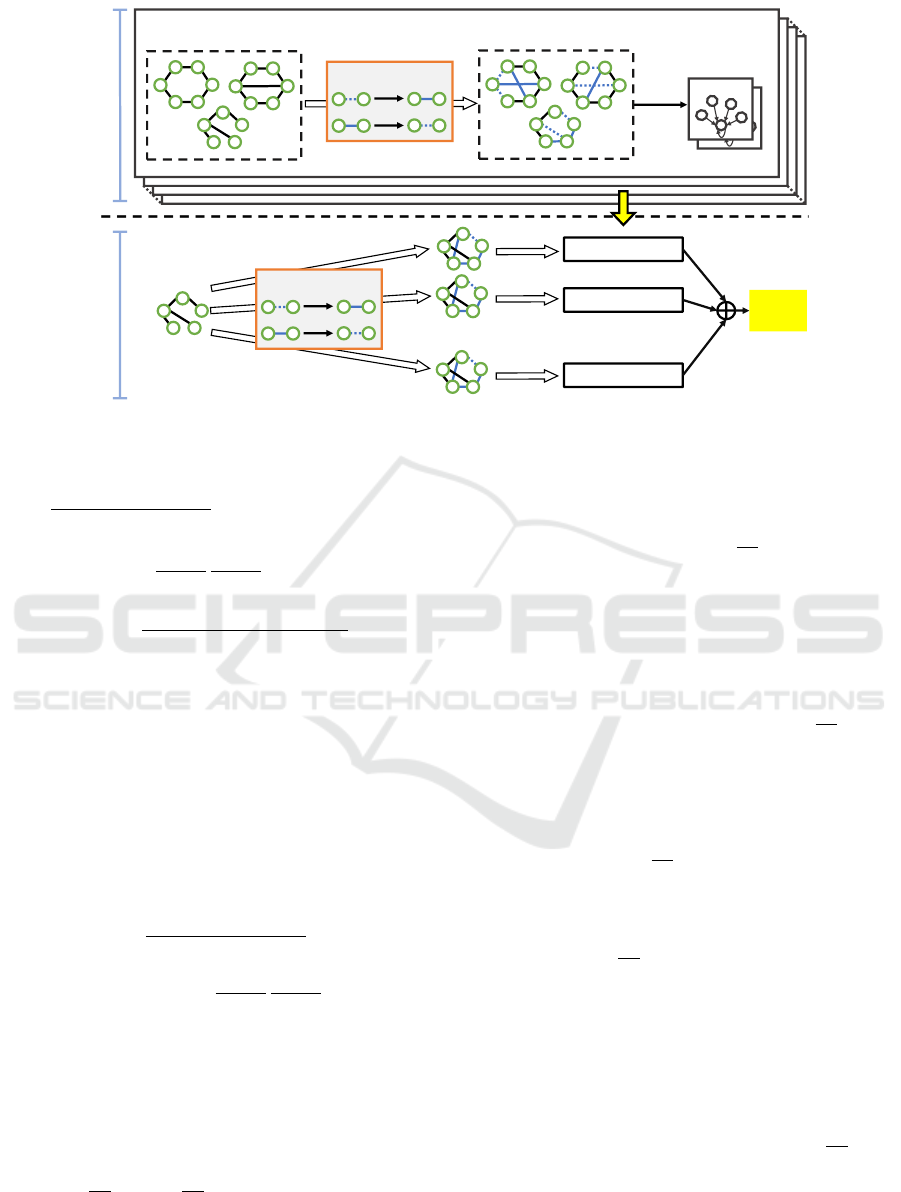
In this section, we explain the algorithm on how to
build a robust model. The outline of this algorithm is
shown in Figure 1.
Algorithm in the Training Phase. First, we de-
scribe the training phase of a binary data classifier.
This section corresponds to lines 1–4 of the Algo-
rithm 1. Our method randomly selects e data from
the entire training dataset D
entire
to create a small sub-
sample dataset D. This subsample extraction is per-
formed independently N times, resulting in N dif-
ferent subsample datasets. Furthermore, defensive
noises are added to the features of the data in the sub-
samples. Here, among the features of the data, ele-
ments of 0 are retained with a probability of β
0
(i.e.,
they are changed to 1 with probability 1 − β
0
), and
elements of 1 are retained with a probability of β
1
(i.e., they are changed to 0 with probability 1 − β
1
).
Each of these randomized subsamples is described as
D ⊕ {ε
i
|1 ≤ i ≤ |D|}. After that, our method prepares
N classifiers. Each of these N models is trained on its
respective randomized subsample and is referred to as
f (D ⊕ {ε
i
|1 ≤ i ≤ |D|}).
Algorithm in the Testing Phase. This section cor-
responds to lines 5–12 in the Algorithm 1. First,
our method adds defensive noise to the features of
each data in the test dataset, similar to the training
phase. Then, the test data x is predicted N times us-
ing the N models. As a result, we obtain N outputs
l = f (x ⊕ ε, D ⊕ {ε
i
|1 ≤ i ≤ |D|}). It is possible to
statistically estimate the top 1 and top 2 label proba-
bilities by counting N
l
A
and N
l
B
, which are the number
of top 1 and top 2 labels in the N outputs, respec-
tively. Finally, based on these results, we derive the
certified radius to theoretically determine the range in
which the model’s predictions remain consistent even
when attack noise is added to the data. The specific
theoretical calculation to obtain the certified radius is
discussed in the following sections.
4.3 Theoretical Calculation
In this section, we describe how to compute the certi-
fied radius using our method to defend against back-
door attacks. To define S
benign
and S
poison
in Eq.(4),
we first calculate P(X = z ∧ D
ε
= D
z
) and P(Y =
z ∧
˜
D
ε
= D
z
). Then, we obtain the likelihood ratio
P(X=z∧D
ε
=D
z
)
P(Y =z∧
˜
D
ε
=D
z
)
. Note that z ∈ {0, 1}
|x|
and D
z
= {d
z,i
∈
{0, 1}
|d
z,i
|
|1 ≤ i ≤ |D|} are elements that could poten-
tially appear after the addition of defensive noise. We
focus on the points where the attack noise is intro-
Algorithm 1: Computing a certified radius.
Input : Train dataset D
entire
, test data x
Output: Certified radius R
x
for x
// Training
1 for i = 1 to N do
2 D ← sample e data from D
entire
3 D ← D ⊕ {ε
i
|1 ≤ i ≤ |D|}
4 f
i
← train( f ,D)
// Testing
5 counter← (0)
L
i=1
6 for i = 1 to N do
7 l ← f
i
(x ⊕ ε) ▷ Label Prediction
8 counter[l]←counter[l]+1
9 N
l
A
←counter[l
A
]
10 N
l
B
←counter[l
B
]
11 calculate p
A
and p
B
on the basis of Eq.(19)
12 R
x
← maximum p or ∥δ∥
0
satisfying Eq.(4)
duced and proceed to calculate
P(X=z∧D
ε
=D
z
)
P(Y =z∧
˜
D
ε
=D
z
)
. Our
method retains elements of 0 in features of test and
training data with probability β
0
, and elements of 1
with probability β
1
. Under this premise, we compute
P(X = z ∧ D
ε
= D
z
) and P(Y = z ∧
˜
D
ε
= D
z
) where
D
ε
and
˜
D
ε
are D ⊕ {ε
i
|1 ≤ i ≤ |D|} and
˜
D ⊕ {ε
i
|1 ≤
i ≤ |D|}, respectively. Among the elements of 0 in
x
tmp
∈ {{x} ∪ D}, considering the positions where the
attack noise is introduced, m
0,i
elements of x
tmp
and
z
tmp
∈ {{z} ∪ D
z
} are the same, while ∥δ
0
∥
0
−m
0,i
el-
ements are different. m
0,0
and m
0,i
(1 ≤ i ≤ |D|) are
assigned to x and d
i
(1 ≤ i ≤ |D|), respectively. Simi-
larly, among the elements of 1 in x
tmp
, m
1,i
elements
of x
tmp
and z
tmp
are the same, while ∥δ
1
∥
0
− m
1,i
ele-
ments are different. These m
i, j
(i ∈ {0, 1}, 1 ≤ j ≤ |D|)
take values in range of [0, ∥δ
i
∥
0
]. δ
0
and δ
1
are the
attack noises that flip the elements of 0 and 1 in
x
tmp
, respectively. Then, P(X = z ∧ D
ε
= D
z
) and
P(Y = z ∧
˜
D
ε
= D
z
) are calculated as
P(X = z ∧ D
ε
= D
z
) =
c
∏
i=0
β
m
0,i
0
(1 − β
0
)
∥δ
0
∥
0
−m
0,i
β
m
1,i
1
(1 − β
1
)
∥δ
1
∥
0
−m
1,i
· p
i
(5)
P(Y = z ∧
˜
D
ε
= D
z
) =
c
∏
i=0
(1 − β
1
)
m
0,i
β
∥δ
0
∥
0
−m
0,i
1
(1 − β
0
)
m
1,i
β
∥δ
1
∥
0
−m
1,i
0
· p
i
.
(6)
p
i
is the probability that, in areas unaffected by attack
noise, the randomized result of x
tmp
matches z
tmp
. The
ICISSP 2025 - 11th International Conference on Information Systems Security and Privacy
556

GNN
model 𝒇
𝟏
input
Randomized
Subsample𝑫
Train
GNNLayer1
Layer1
Inference phase
Training phase
GNN model 𝒇
𝟏
GNN model 𝒇
𝟐
GNN model 𝒇
𝑵
･･･
･･･
Count
Output
･･･
･･･
𝟏 − 𝜷
𝟎
𝟏 − 𝜷
𝟏
Defensive noise
𝟏 − 𝜷
𝟎
𝟏 − 𝜷
𝟏
Defensive noise
Subsample 𝑫
Figure 1: Overview of constructing a robust model through our method.
likelihood ratio is formulated as
P(X = z ∧ D
ε
= D
z
)
P(Y = z ∧
˜
D
ε
= D
z
)
=
C
c+1
·

β
0
1 − β
0
β
1
1 − β
1

∑
c
i=0
(m
0,i
+m
1,i
)
where C =
(1 − β
0
)
∥δ
0
∥
0
(1 − β
1
)
∥δ
1
∥
0
β
∥δ
1
∥
0
0
β
∥δ
0
∥
0
1
.
(7)
There are 2c + 2 variables, m
0,i
and m
1,i
. However,
since they are consolidated in the exponent, we treat
their sum as a single variable. That is, we introduce
a new variable m, where m =
∑
c
i=0
(m
0,i
+ m
1,i
). This
m represents the total number of different elements
between (x, D) and (z, D
z
). Based on this likelihood
ratio, we define a fundamental set R(c, m) as
R(c, m) =

(z, D
z
)




|D|
∑
i=1
I[D
ε,i
̸=
˜
D
ε,i
] = c ∧
P(X = z ∧ D
ε
= D
z
)
P(Y = z ∧
˜
D
ε
= D
z
)
= r(c, m)

,
where r(c, m) = C
c+1
·

β
0
1 − β
0
β
1
1 − β
1

m
.
(8)
We construct the set S
benign
based on this basic set.
Considering the premise of P(h(X) = 1) ≥ P(X ∈
S
benign
), the set S
benign
represents the lower bound of
the probability that the classifier h returns the cor-
rect probability for benign data. Therefore, P(X ∈
S
benign
) = p
A
, where p
A
is the lower bound of the
probability that the classifier outputs label l
A
. Calcu-
lating P(h(X) = 1) directly requires complex compu-
tations depending on the model h. However, the lower
bound can actually be estimated relatively easily us-
ing Monte Carlo sampling. While the specific method
for calculating this lower bound is described later, we
proceed with the assumption that p
A
is a known value.
We build S
benign
on the basis of R(c, m) from here.
Let R
i
be sorted in descending order according to the
likelihood ratio r(c, m), and S
benign
is defined as
S
benign
=
[
1≤i≤a
∗
R
i
∪ R
sub
,
s.t. a
∗
= argmax
a
a
∑
i=1
P((X, D
ε
) ∈ R
i
) ≤ p
A
.
(9)
S
sub
is a set defined as
S
sub
⊆ R
a
∗
+1
∧
P((X, D
ε
) ∈ S
sub
) = p
A
−
a
∗
∑
i=1
P((X, D
ε
) ∈ R
i
).
(10)
In the Neyman-Pearson lemma, S
sub
corresponds to
the set S
3
and P((X , D
ε
) ∈ S
benign
) is adjusted so that
it exactly matches p
A
. S
benign
is a set that selects a por-
tion of data with highest likelihood ratio. S
benign
can
be interpreted as a collection of samples that appear
to be the most benign.
We can now compute P((X, D
ε
) ∈ S
benign
) and
P((Y,
˜
D
ε
) ∈ S
benign
). Obviously, P((X, D
ε
) ∈ S
benign
)
is formulated as
a
∗
∑
i=1
P((X, D
ε
) ∈ R
i
) + P((X, D
ε
) ∈ R
sub
) = p
A
.
(11)
Then, we compute P((Y,
˜
D
ε
) ∈ S
benign
). P((Y,
˜
D
ε
) ∈
S
benign
) represents the probability that, when defen-
sive noise is added to poisoned data, it matches the
Flexible Noise Based Robustness Certification Against Backdoor Attacks in Graph Neural Networks
557

most benign-looking data, (z, D
z
), in S
benign
. Sim-
ilar to the case of P((X, D
ε
) ∈ S
benign
), P((Y,
˜
D
ε
) ∈
S
benign
) is formulated as
a
∗
∑
i=1
P((Y,
˜
D
ε
) ∈ R
i
) +
P((X, D
ε
) ∈ R
sub
)
r
a
∗
+1
. (12)
The final term is divided by the likelihood ratio r
a
∗
+1
of S
sub
. This is easier to understand when recalling the
definition of the likelihood ratio, and can be derived
from r
a
∗
+1
=
P(X=z∧D
ε
=D
z
)
P(Y =z∧
˜
D
ε
=D
z
)
to
P((X, D
ε
) ∈ R
sub
)
r
a
∗
+1
=
P((X, D
ε
) ∈ R
sub
)
P(X=z∧D
ε
=D
z
)
P(Y =z∧
˜
D
ε
=D
z
)
= P(Y = z ∧
˜
D
ε
= D
z
) ·
P((X, D
ε
) ∈ R
sub
)
P((X, D
ε
) ∈ R
sub
)
= P(Y = z ∧
˜
D
ε
= D
z
) ·
|R
sub
| · P((X, D
ε
) ∈ R
sub
)
P((X, D
ε
) ∈ R
sub
)
= P(Y = z ∧
˜
D
ε
= D
z
) · |R
sub
|
= P((Y,
˜
D
ε
) ∈ R
sub
).
(13)
This term, unlike the others involving P((Y,
˜
D
ε
) ∈ R
i
),
forms a truncated set, which makes it mathematically
difficult to count. Therefore, it is simply expressed in
a form using the more easily obtainable P((X , D
ε
) ∈
R
sub
).
Next, we calculate P((X, D
ε
) ∈ S
benign
) and
P((Y,
˜
D
ε
) ∈ S
benign
) using combinatorial formulas and
exponentiation. Given that R
i
is a set of rearranged
R(c, m), it suffices to compute P((X, D
ε
) ∈ R(c, m))
and P((Y,
˜
D
ε
) ∈ R(c, m)) for any non-negative integer
m. Therefore, we proceed with these calculations.
Then, P((X, D
ε
) ∈ R(c, m)) and P((Y,
˜
D
ε
) ∈
R(c, m)) are formulated as
P((X, D
ε
) ∈ R(c, m)) =

p
c

n−p
e−c


n
e

∑
∑
c
i=0
(m
0,i
+m
1,i
)=m
c
∏
i=0

∥δ
0
∥
0
m
0,i

∥δ
1
∥
0
m
1,i

×
β
m
0,i
0
(1 − β
0
)
∥δ
0
∥
0
−m
0,i
β
m
1,i
1
(1 − β
1
)
∥δ
1
∥
0
−m
1,i

,
(14)
P((Y,
˜
D
ε
) ∈ R(c, m)) =

p
c

n−p
e−c


n
e

∑
∑
c
i=0
(m
0,i
+m
1,i
)=m
c
∏
i=0

∥δ
0
∥
0
m
0,i

∥δ
1
∥
0
m
1,i

×
(1 − β
1
)
m
0,i
β
∥δ
0
∥
0
−m
0,i
1
(1 − β
0
)
m
1,i
β
∥δ
1
∥
0
−m
1,i
0

(15)
The formulation for the probability calculation is
complete. However, performing this calculation di-
rectly requires a very high computational cost because
there are many variables. Therefore, following the
method used by (Zhang et al., 2022), we reduce the
computational cost based on a recurrence relation.
We define T (c, m) as follows and derive a recur-
rence relation.
T (c, m)
=
∑
∑
c
i=0
(m
0,i
+m
1,i
)=m
c
∏
i=0
p(m
0,i
, m
1,i
)
=
∑
0≤m
c
≤∥δ∥
0
∑
m
0,c
+m
1,c
=m
c
∑
∑
c−1
i=0
(m
0,i
+m
1,i
)
=m−m
c
c
∏
i=0
p(m
0,i
, m
1,i
)
=
∑
0≤m
c
≤|δ|
(
∑
m
0,c
+m
1,c
=m
c
p(m
0,c
, m
1,c
)×
∑
∑
c−1
i=0
(m
0,i
+m
1,i
)=m−m
c
c−1
∏
i=0
p(m
0,i
, m
1,i
)
)
=
∑
0≤m
c
≤∥δ∥
0
T (0, m
c
) · T (c − 1, m − m
c
),
(16)
where
p(m
0
, m
1
) =

∥δ
0
∥
0
m
0

∥δ
1
∥
0
m
1

×
β
m
0
0
(1 − β
0
)
∥δ
0
∥
0
−m
0
β
m
1
1
(1 − β
1
)
∥δ
1
∥
0
−m
1
(17)
Then, we have
T (c, m) =
∑
0≤m
c
≤∥δ∥
0
T (0, m
c
) · T (c − 1, m − m
c
).
(18)
This allows us to compute any T (c, m) from the recur-
rence relation in O(e
2
∥δ∥
2
0
) time, once the initial val-
ues T (0, m
c
) for 0 ≤ m
c
≤ ∥δ∥
0
are calculated. Since
P((X, D
ε
) ∈ R(c, m)) is a constant multiple of T (c, m),
we can also compute P((X, D
ε
) ∈ R(c, m)) from the
above. The calculation of P((Y,
˜
D
ε
) ∈ R(c, m)) is the
same as P((X, D
ε
) ∈ R(c, m)).
Note that we need two noise size, ∥δ
0
∥
0
and
∥δ
1
∥
0
, to calculate the probabilities although exist-
ing methods need only ∥δ∥
0
= ∥δ
0
∥
0
+ ∥δ
1
∥
0
. When
calculating all combinations of ∥δ
0
∥
0
and ∥δ
1
∥
0
that
satisfy ∥δ∥
0
= ∥δ
0
∥
0
+ ∥δ
1
∥
0
, the computational cost
increases. Therefore, in the results of this paper, we
first identify the worst-case ∥δ
0
∥ and ∥δ
1
∥ that sat-
isfy ∥δ∥
0
= ∥δ
0
∥
0
+ ∥δ
1
∥
0
and report on the results
for this worst case. To be specific, for all ∥δ
0
∥
0
and
∥δ
1
∥
0
such that ∥δ∥
0
= ∥δ
0
∥
0
+∥δ
1
∥
0
, we compute C
in Eq.(7) and adopt the ∥δ
0
∥
0
and ∥δ
1
∥
0
for which C
is maximized as the worst-case noise.
ICISSP 2025 - 11th International Conference on Information Systems Security and Privacy
558

4.4 Estimate p
A
and p
B
We estimate p
A
and p
B
according to the methodol-
ogy described in (Jia et al., 2019). In our method,
we obtain the output according to the formula, l =
g(x, D) = f (x ⊕ ε, D ⊕ {ε
i
|1 ≤ i ≤ |D|}). For a spe-
cific label l, we assume that P(g(x, D) = l) = p
l
. Fur-
thermore, the operation of selecting a subsample D
from D
entire
and the generation of ε and ε
i
are carried
out independently. Therefore, N
l
=
∑
N
i=1
I[g(x, D) = l]
follows a binomial distribution with the number of tri-
als N and success probability p
l
. From the above, the
lower bound p
A
for the probability p
A
of outputting
l
A
and the upper bound p
B
for the probability p
B
of
outputting l
B
are estimated as
p
A
= Beta

α
L
;N
l
A
, N − N
l
A
+ 1

,
p
B
= min

Beta

1 −
α
L
;N
l
B
+ 1, N − N
l
B

, 1 − p
A

(19)
where α and L represent the significance level and the
number of classes. Note that a Bonferroni correction
is applied to the significance level in Eq.(19), which
means dividing it by the number of test data |D
test
|.
By setting α =
α
entire
|D
test
|
for each test data, α
entire
for the
entire test dataset is achieved. We set α
entire
= 5% in
our experiment.
5 EVALUATION
In this section, we show the results of the baseline and
our method. The results of the baseline correspond
to the existing method (Zhang et al., 2022) applied
to a binary data classifier. Note that we do not ap-
ply the existing method as-is. In the evaluation of the
baseline in this paper, the ensemble learning dataset
is created using non-replacement sampling, and the
probability calculations for deriving certified radius
are focused solely on the locations where attack noise
is introduced as described in section 4.3. This is be-
cause we conduct a fair comparison with the baseline
and evaluate the effectiveness of the flexible noise.
In this experiment, we aim to address the follow-
ing questions.
1. Is the flexible defensive noise of our method ef-
fective in improving the robustness certification?
2. What combinations of β
0
and β
1
in our method
are suitable for each dataset?
3. How does the level of robustness vary if the poi-
soning size is changed?
4. How does the level of robustness vary if the attack
noise size is changed?
5.1 Settings
Datasets. We evaluate the robustness of graph neu-
ral networks on MUTAG (Debnath et al., 1991),
DHFR (Wale et al., 2008), NCI1 (Dobson and Doig,
2003) and AIDS (Riesen and Bunke, 2008) datasets.
The MUTAG and DHFR datasets are split into train-
ing and test data with a ratio of 8:2. For the NCI1 and
AIDS datasets, experiments are conducted with 250
training data and 50 test data for each label which are
randomly chosen from the original datasets.
In our experiments, e, the size of the ensemble
learning dataset D, is set to 50 for all datasets.
Models. We conduct experiments on graph convo-
lutional networks (GCNs) (Kipf and Welling, 2016).
Our model consists of two GCN layers and one linear
classifier.
Metrics. We use certified accuracy (CA) for our
evaluation. CA indicates the proportion of test data
for which the prediction remains unchanged and the
correct label is output, even if data are changed by the
attacker. This metric is designed to evaluate both the
performance and robustness of the model. In the cer-
tification of backdoor attacks, when evaluating CA,
two axes can be considered. The first axis is the num-
ber of poisons p in the training dataset. In this case,
the number of attack noise inserted into each poisoned
data, ∥δ∥
0
, is fixed at a constant value, and CA is eval-
uated while varying p. In particular, we describe CA
at poisoning size p as CA
p
. The second axis is the
number of attack noise. In this case, p is fixed at
a constant value and CA is evaluated while varying
∥δ∥
0
. Specifically, we describe the CA at attack noise
size ∥δ∥
0
as CA
∥δ∥
0
.
Then, CA
p
and CA
∥δ∥
0
are formulated as
CA
p
=
∑
|D
test
|
i=1
I

R
x
≥ p ∧ l = l
∗

|D
test
|
and
CA
∥δ∥
0
=
∑
|D
test
|
i=1
I

R
x
≥ ∥δ∥
0
∧ l = l
∗

|D
test
|
where l
∗
= arg max
l∈{1,...,L}

N
∑
i=1
I[g(x, D) = l]

,
(20)
respectively. The range of p and ∥δ∥
0
are [0, |D
entire
|]
and [0, 100] in our experiments, respectively.
Explore the Optimal β
0
and β
1
. We conduct the
evaluation for large-size certification (N = 1000) af-
ter exploring the optimal value of the defensive noise
through a heuristic approach using small-size certifi-
cation (N = 100). In the existing method, evaluations
Flexible Noise Based Robustness Certification Against Backdoor Attacks in Graph Neural Networks
559

are conducted while varying the value of β. However,
large-size certification requires a significant compu-
tational cost in our method, making it difficult to try
various combinations of defensive noise probabilities.
Therefore, we simplify the computation by optimiz-
ing the probability of defensive noise based on small-
size certification in advance. We define the average
certified radius, R, for the test dataset as
R
poison
=
p
max
∑
p=0
p · (CA
p
−CA
p+1
),
R
noise
=
∥δ∥
max
0
∑
∥δ∥
0
=0
∥δ∥
0
· (CA
∥δ∥
0
−CA
∥δ∥
0
+1
)
(21)
for poisoning size and noise size certification, respec-
tively. CA
p
max
+1
and CA
∥δ∥
max
0
+1
are set to 0.
We report the results for large-size certification
where the value of R
poison
is maximized in small-size
certification. In the small-size certification, we calcu-
late the R
poison
where ∥δ∥
0
= 1. In the certification
of the baseline, we search for the optimal β in incre-
ments of 0.1 within the range of β = 0.6 to 0.9, sat-
isfying β
0
= β
1
= β. In our method, we search for
the optimal values of β
0
and β
1
separately in incre-
ments of 0.1 within the range of 0.2 to 0.9, satisfying
β
0
+ β
1
> 1. Note that when β
0
+ β
1
= 1, data are
completely randomized and P(X = z ∧ D
ε
= D
z
) =
P(Y = z ∧
˜
D
ε
= D
z
). Thus, the model becomes com-
pletely unaffected by attack noise.
5.2 Experimental Results
Results for Poisoning Size. In this section, we re-
port the results for poisoning size certification. This
experiment confirms the model’s robustness against
backdoor attacks that inject p poison into the training
dataset. We vary the poisoning size p in the range
from 0 to |D
entire
| where the attack noise size ∥δ∥
0
is
1, 5, and 10. Fig. 2 and Fig. 3 shows the CA as a
function of p in the baseline and our method, respec-
tively. As can be seen from Fig. 2 and Fig. 3, on the
all datasets, our method can maintain high CA against
backdoor attacks with large poisoning size compared
with the baseline.
In the MUTAG dataset, when focusing on the case
where ∥δ∥
0
= 1 (the blue line in Fig. 2(a)), the base-
line demonstrates 63.15% CA when p is 10. In con-
trast, our method maintains a high CA, achieving
71.05% when the poisoning size is 10 as shown in
Fig. 3(a). Furthermore, even in the other situations
where noise sizes are 5 and 10, our method outper-
forms the baseline. For example, in the case where
the noise size is 10 as shown in the green line in
Fig. 2(a), the CA of the baseline is already 0 when
the poisoning size is 20 . On the other hand, our
method maintains approximately 20% CA as shown
in Fig. 3(a). As a clearer indicator, R
poison
shows
that the baseline has 34.10, 5.57, 2.07 and our method
has 81.73, 20.34, 9.44 on ∥δ∥
0
= 1, 5, 10, demonstrat-
ing the usefulness of the guarantees provided through
flexible noise.
In the DHFR dataset, in the case where ∥δ∥
0
= 1
(the blue line in Fig. 2(b)), the baseline demonstrates
18.42% CA against poisoning attacks whose poison-
ing size is 10. In contrast, our method achieves
40.13% with the same poisoning size as shown in
Fig. 3(b). Furthermore, our method retains more
than 0% CA with larger poisoning sizes. Regard-
ing the average certified radius, R
poison
shows that
the baseline has 7.87, 0.37, 0.00 and our method has
71.38, 11.06, 4.05 on ∥δ∥
0
= 1, 5, 10.
In the NCI1 dataset, the baseline demonstrates
13% CA when the poisoning size is 10, in the case
where ∥δ∥
0
= 1 as shown in the blue line in Fig. 2(c).
In contrast, our method achieves 16% CA at the same
poisoning size as shown in Fig. 3(c). The difference in
CA between our method and the baseline is relatively
small compared with the results on other datasets.
However, our method can maintain more than 0%
CA even at larger poisoning sizes as with results on
other datasets. Regarding the average certified radius,
R
poison
shows that the baseline has 4.55, 0.16, 0.00 and
our method has 8.85, 0.82, 0.05 on ∥δ∥
0
= 1, 5, 10.
Finally, in the AIDS dataset, the baseline demon-
strates 80% CA when the poisoning size is 100
as shown in the blue line in Fig. 2(d). In con-
trast, our method achieves approximately 90% CA
when the poisoning size is 10 as shown in the blue
line in Fig. 3(d). It is noteworthy that our method
can keep approximately 80% CA even when the
poisoning size is 500 whereas the CA of baseline
is dropped to 0% when the size is 250. As for
the other cases, our method maintains higher CA
with larger poisoning sizes as shown in the orange
and green lines in Fig. 3(d). Regarding the av-
erage certified radius, R
poison
shows that the base-
line has 198.08, 44.72, 18.88 and our method has
423.33, 200.05, 96.52 on ∥δ∥
0
= 1, 5, 10.
The experimental results confirm that, in general,
applying our flexible noise significantly improves the
model’s robustness compared to adding defensive
noise to each edge with the same probability. Addi-
tionally, for the MUTAG dataset, the model remains
robust at high poisoning levels, when existing edges
are removed with high probability. Therefore, if the
defender would like to ensure correct predictions un-
der large-scale poisoning attacks, defensive noise that
deletes existing edges with high probability should be
ICISSP 2025 - 11th International Conference on Information Systems Security and Privacy
560

(a) MUTAG
(β
0
= β
1
= 0.6)
(b) DHFR
(β
0
= β
1
= 0.6)
(c) NCI1
(β
0
= β
1
= 0.6)
(d) AIDS
(β
0
= β
1
= 0.6)
Figure 2: CA as a function of the poisoning size in the baseline.
(a) MUTAG
(β
0
= 0.8, β
1
= 0.3)
(b) DHFR
(β
0
= 0.3, β
1
= 0.8)
(c) NCI1
(β
0
= 0.2, β
1
= 0.9)
(d) AIDS
(β
0
= 0.6, β
1
= 0.5)
Figure 3: CA as a function of the poisoning size in our method.
applied. On the other hand, for the DHFR and NCI1
datasets, defensive noise should focus on changing
the elements of 0 in the adjacency matrix to 1 with
high probability. Regarding the AIDS dataset, the op-
timal approach is to apply defense noise in a way that
maintains more than half of the 0 and 1 edges. In
this case, the defense noise is relatively similar to the
baseline. However, it is remarkable that a 10% change
in defensive noise probability results in such a signif-
icant improvement in robustness.
Results for Noise Size. We also report the results
for the noise size certification in this section. This
experiment confirms the model’s robustness against
backdoor attacks when ∥δ∥
0
edges of each graph data
are changed. We vary the attack noise size ∥δ∥
0
in
the range from 0 to 100. We evaluate the performance
of the baseline and our method through varying the
poisoning size p to 0, 5, and 15. Here, p = 0 is the
same situation as evasion attacks. When evaluation
is conducted while varying the noise size, the data
size is normally required. However, in this paper,
we intentionally disregard the data size in the evalua-
tion. This is because our method can certify how the
model is robust even when the attack range is larger
than the size of data. For example, our method may
compute a certified radius of 30 for data with a size
of 25. In this case, we interpret it as meaning that
our model’s robustness has a surplus equivalent to 5
attack noises, and we directly reflect this in the CA
evaluation. Fig. 4 and Fig. 5 shows the CA as a func-
tion of the noise size in the baseline and our method,
respectively. As can be seen from Fig. 4 and Fig. 5,
our method can retain higher CA on the all datasets
with large noise sizes compared with the baseline.
In the MUTAG dataset, when focusing on the
case where p = 5 (orange line in Fig. 4(a)), the
baseline demonstrates 15.78% CA when noise is
10. On the othe hand, our method achieves 55.26%
at the same noise size as shown in orange line in
Fig. 5(a). Additionally, our method can maintain
higher CA until the noise size exceeds 40 whereas
the CA of the baseline is 0% before the noise size
is 20. Even in the case where p = 0 and 10, the re-
sults demonstrate that our method is effective. Re-
garding the average certified radius,
R
noise
shows that
the baseline has 11.86, 4.23, 1.73 and our method has
36.39, 13.78, 5.86 on p = 0, 5, 15.
In the DHFR dataset, the CA of the baseline is 0%
when the noise size exceeds 10 in the all cases. In
particular, in the case where poisoning size is 15, the
baseline demonstrates 0% CA when the noise size is
10 as shown in the green line in Fig. 4(b). In contrast,
our method achieves 19.73% as shown in the green
line in Fig. 5(b). Furthermore, our method retains
higher CA with larger noise sizes compared with the
baseline in all the cases. In this dataset, R
noise
shows
that the baseline has 0.94, 0.53, 0.25 and our method
has 6.36, 4.47, 2.75 on p = 0, 5, 15.
In the NCI1 dataset, the baseline shows results
similar to those on DHFR. For example, the base-
line demonstrates 0% CA when the noise size is 5
as shown in the orange line in Fig. 4(c). In contrast,
our method achieves 9.00% CA at the same noise size
Flexible Noise Based Robustness Certification Against Backdoor Attacks in Graph Neural Networks
561

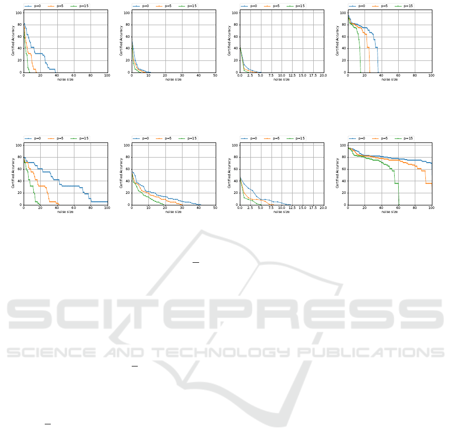
(a) MUTAG
(β
0
= β
1
= 0.6)
(b) DHFR
(β
0
= β
1
= 0.6)
(c) NCI1
(β
0
= β
1
= 0.6)
(d) AIDS
(β
0
= β
1
= 0.6)
Figure 4: CA as a function of the noise size in the baseline (β
0
= β
1
= 0.6).
(a) MUTAG
(β
0
= 0.8, β
1
= 0.3)
(b) DHFR
(β
0
= 0.3, β
1
= 0.8)
(c) NCI1
(β
0
= 0.2, β
1
= 0.9)
(d) AIDS
(β
0
= 0.6, β
1
= 0.5)
Figure 5: CA as a function of the noise size in our method.
in the orange line in Fig. 5(c). In this dataset, R
noise
shows that the baseline has 0.23, 0.10, 0.03 and our
method has 1.41, 0.65, 0.30 on p = 0, 5, 15.
Finally, in the AIDS dataset, when we focus on the
case where the poisoning size is 15, our method main-
tains 73.00% CA when the noise size is 40 as shown
in the green line in Fig. 5(d). On the other hand, the
CA of the baseline is already 0% at the same noise
size as shown in the green line in Fig. 4(d). Regard-
ing the average certified radius,
R
noise
shows that the
baseline has 25.55, 18.05, 10.24 and our method has
79.93, 72.74, 43.52 on p = 0, 5, 15.
From the above results, it is confirmed that ex-
panding the search range for defense noise also im-
proves the R
noise
.
6 CONCLUSION
We have proposed a new robustness certification
method against backdoor attacks in the graph domain
by introducing flexible noise. As a result, the defender
can explore a wider range of defensive noise parame-
ters, allowing for more flexible handling against data
modification attacks. Additionally, our method can
use training datasets that include data of different
sizes, providing a clear certification framework for
classifiers that categorize a wide range of data types.
In terms of computational complexity, our method is
more efficient due to focusing calculations only on lo-
cations where attack noises are present. Our results
demonstrate that adding flexible noise to binary ele-
ments is effective in improving the level of robustness
certification.
Limitations and Future Work. However, our
method has two limitations. First, our method is in-
tended only for binary data classifiers among discrete
data classifiers. Therefore, providing flexible robust-
ness certification for other classifiers is a future chal-
lenge. Second, in this paper, we optimized the de-
fensive noise based on the average certified radius.
However, there are other possible approaches such as
optimization based on CA with a certain poisoning
or noise size. Therefore, it is also necessary to ex-
plore more practical optimization methods for use in
robustness certification.
We hope that our flexible noise based robustness
certification will inspire research on broader guaran-
tees for discrete data classifiers in future.
REFERENCES
Chen, L., Li, J., Peng, J., Xie, T., Cao, Z., Xu, K., He, X.,
Zheng, Z., and Wu, B. (2020). A survey of adversarial
learning on graphs. arXiv preprint arXiv:2003.05730.
Cohen, J., Rosenfeld, E., and Kolter, Z. (2019). Certified
adversarial robustness via randomized smoothing. In
international conference on machine learning, pages
1310–1320. PMLR.
Debnath, A. K., Lopez de Compadre, R. L., Debnath, G.,
Shusterman, A. J., and Hansch, C. (1991). Structure-
activity relationship of mutagenic aromatic and het-
eroaromatic nitro compounds. correlation with molec-
ICISSP 2025 - 11th International Conference on Information Systems Security and Privacy
562

ular orbital energies and hydrophobicity. Journal of
medicinal chemistry, 34(2):786–797.
Dobson, P. D. and Doig, A. J. (2003). Distinguishing
enzyme structures from non-enzymes without align-
ments. Journal of molecular biology, 330(4):771–
783.
Feng, P., Ma, J., Li, T., Ma, X., Xi, N., and Lu, D.
(2020). Android malware detection based on call
graph via graph neural network. In 2020 International
Conference on Networking and Network Applications
(NaNA), pages 368–374. IEEE.
Goodfellow, I. J., Shlens, J., and Szegedy, C. (2014). Ex-
plaining and harnessing adversarial examples. arXiv
preprint arXiv:1412.6572.
Gu, T., Dolan-Gavitt, B., and Garg, S. (2019). Bad-
nets: Identifying vulnerabilities in the machine learn-
ing model supply chain.
Guo, L., Yin, H., Chen, T., Zhang, X., and Zheng, K.
(2021). Hierarchical hyperedge embedding-based
representation learning for group recommendation.
ACM Transactions on Information Systems (TOIS),
40(1):1–27.
Jia, J., Cao, X., and Gong, N. Z. (2021). Intrinsic certified
robustness of bagging against data poisoning attacks.
In Proceedings of the AAAI conference on artificial
intelligence, volume 35, pages 7961–7969.
Jia, J., Cao, X., Wang, B., and Gong, N. Z. (2019). Cer-
tified robustness for top-k predictions against adver-
sarial perturbations via randomized smoothing. arXiv
preprint arXiv:1912.09899.
Jiang, B. and Li, Z. (2022). Defending against backdoor at-
tack on graph nerual network by explainability. arXiv
preprint arXiv:2209.02902.
Jiang, C., He, Y., Chapman, R., and Wu, H. (2022). Cam-
ouflaged poisoning attack on graph neural networks.
In Proceedings of the 2022 International Conference
on Multimedia Retrieval, pages 451–461.
Kipf, T. N. and Welling, M. (2016). Semi-supervised clas-
sification with graph convolutional networks. arXiv
preprint arXiv:1609.02907.
Kwon, H., Yoon, H., and Park, K.-W. (2019). Selec-
tive poisoning attack on deep neural network to in-
duce fine-grained recognition error. In 2019 IEEE
Second International Conference on Artificial Intel-
ligence and Knowledge Engineering (AIKE), pages
136–139. IEEE.
Liu, Z., Chen, C., Yang, X., Zhou, J., Li, X., and Song,
L. (2020). Heterogeneous graph neural networks for
malicious account detection.
Meguro, R., Kato, H., Narisada, S., Hidano, S., Fukushima,
K., Suganuma, T., and Hiji, M. (2024). Gradient-
based clean label backdoor attack to graph neural net-
works. In ICISSP, pages 510–521.
Qiu, R., Huang, Z., Li, J., and Yin, H. (2020). Exploiting
cross-session information for session-based recom-
mendation with graph neural networks. ACM Trans-
actions on Information Systems (TOIS), 38(3):1–23.
Riesen, K. and Bunke, H. (2008). Iam graph database repos-
itory for graph based pattern recognition and machine
learning. In Structural, Syntactic, and Statistical Pat-
tern Recognition: Joint IAPR International Workshop,
SSPR & SPR 2008, Orlando, USA, December 4-6,
2008. Proceedings, pages 287–297. Springer.
Shafahi, A., Huang, W. R., Najibi, M., Suciu, O., Studer,
C., Dumitras, T., and Goldstein, T. (2018). Poison
frogs! targeted clean-label poisoning attacks on neural
networks. Advances in neural information processing
systems, 31.
Wale, N., Watson, I. A., and Karypis, G. (2008). Compar-
ison of descriptor spaces for chemical compound re-
trieval and classification. Knowledge and Information
Systems, 14:347–375.
Wang, B., Jia, J., Cao, X., and Gong, N. Z. (2021). Certified
robustness of graph neural networks against adversar-
ial structural perturbation. In Proceedings of the 27th
ACM SIGKDD Conference on Knowledge Discovery
& Data Mining, pages 1645–1653.
Wang, S., Chen, Z., Ni, J., Yu, X., Li, Z., Chen, H., and Yu,
P. S. (2019). Adversarial defense framework for graph
neural network. arXiv preprint arXiv:1905.03679.
Weber, M., Xu, X., Karla
ˇ
s, B., Zhang, C., and Li, B. (2023).
Rab: Provable robustness against backdoor attacks. In
2023 IEEE Symposium on Security and Privacy (SP),
pages 1311–1328. IEEE.
Yang, J., Ma, W., Zhang, M., Zhou, X., Liu, Y., and Ma, S.
(2021). Legalgnn: Legal information enhanced graph
neural network for recommendation. ACM Transac-
tions on Information Systems (TOIS), 40(2):1–29.
Zhang, M., Hu, L., Shi, C., and Wang, X. (2020). Adversar-
ial label-flipping attack and defense for graph neural
networks. In 2020 IEEE International Conference on
Data Mining (ICDM), pages 791–800. IEEE.
Zhang, X. and Zitnik, M. (2020). Gnnguard: Defend-
ing graph neural networks against adversarial attacks.
Advances in neural information processing systems,
33:9263–9275.
Zhang, Y., Albarghouthi, A., and D’Antoni, L. (2022).
Bagflip: A certified defense against data poisoning.
Advances in Neural Information Processing Systems,
35:31474–31483.
Zhang, Z., Jia, J., Wang, B., and Gong, N. Z. (2021). Back-
door attacks to graph neural networks. In Proceedings
of the 26th ACM Symposium on Access Control Mod-
els and Technologies, pages 15–26.
Z
¨
ugner, D., Akbarnejad, A., and G
¨
unnemann, S. (2018).
Adversarial attacks on neural networks for graph data.
In Proceedings of the 24th ACM SIGKDD interna-
tional conference on knowledge discovery & data
mining, pages 2847–2856.
Flexible Noise Based Robustness Certification Against Backdoor Attacks in Graph Neural Networks
563