Industrial Image Grouping Through Pre-Trained CNN Encoder-Based

Feature Extraction and Sub-Clustering

Selvine G. Mathias

, Saara Asif

, Muhammad Uzair Akmal

, Simon Knollmeyer

Leonid Koval

and Daniel Grossmann

AImotion Bavaria, Technische Hochschule Ingolstadt, Esplanade 10, 85049 Ingolstadt, Germany

{SelvineGeorge.Mathias, Saara.Asif, MuhammadUzair.Akmal, Simon.Knollmeyer, Leonid.Koval,

Daniel.Grossmann}@thi.de

Keywords:

Clustering, CNN Encoder, Convergence, C-Score.

Abstract:

A common challenge faced by many industries today is the classiﬁcation of unlabeled image data from produc-

tion processes into meaningful groups or patterns for better documentation and analysis. This paper presents a

sequential approach for leveraging industrial image data to identify patterns in products or processes for plant

ﬂoor operators. The dataset used is sourced from steel production, and the model architecture integrates fea-

ture reduction through convolutional neural networks (CNNs) like VGG, EfﬁcientNet, and ResNet, followed

by clustering algorithms to assign appropriate labels to the observed data. The model’s selection criteria com-

bine clustering metrics, including entropy minimization and silhouette score maximization. Once primary

clusters are identiﬁed, sub-clustering is performed using near-labels, which are pre-assigned to images with

initial distinctions. A novel metric, C-Score, is introduced to assess cluster convergence and grouping accu-

racy. Experimental results demonstrate that this method can address challenges in detecting variations across

images, improving pattern recognition and classiﬁcation.

1 INTRODUCTION

Raw data in many plant ﬂoors tends to be unlabeled,

nasty, and unstructured due to erroneous data record-

ing and machine or robot failures. Despite these

challenges, any data arriving from the plant ﬂoors,

whether from machines directly or databases record-

ing these observational values, constitutes a readily

available source of information to work upon. One

of the important problems in investigating data is to

know the class or category or label of the data (Xu

and Tian, 2015; Xu and Wunsch, 2005). This is done

by manual inspection in most cases which is time-

consuming, inefﬁcient, and downtime-inducing. Hav-

ing a category for the samples gives usable knowl-

edge for further analysis such as classiﬁcations. How-

ever, no standard methodology is available to ob-

tain them. This paper proposes a simple yet effec-

https://orcid.org/0000-0002-6549-0763

https://orcid.org/0009-0006-1284-5635

https://orcid.org/0009-0007-3961-1174

https://orcid.org/0009-0002-1429-6992

https://orcid.org/0000-0003-4845-6579

https://orcid.org/0000-0002-7388-5757

tive scheme of grouping obtained high-dimensional

samples into clusters based on feature reductions em-

ployed by transfer learning (TF) techniques (Cardoso

and Ferreira, 2021; Silva and Capretz, 2019).

This research varies from the current literature

in two aspects: 1) The proposed scheme presents a

pipe-lining of readily available algorithms to tackle

labeling issues and 2) this research focuses more on

the end-user application, rather than performance for

leveraging the ability to generalize this scheme across

different types of image datasets. For this study, a

public dataset has been used for comparisons of the

working of the model. This paper has been divided

into the following sections: Section 2 discusses the

prevalent applications in the literature focusing on

clustering, artiﬁcial neural networks (ANNs), and TF

approaches. Sections 3 and 4 describe the proposed

methodology and its implementation details. Sec-

tion 5 presents a discussion of the performance of

the models across the different algorithms along with

some observations. The ﬁnal sections present an end-

to-end view of such an application on the production

ﬂoor and conclude with some brief thoughts on future

works.

496

Mathias, S. G., Asif, S., Akmal, M. U., Knollmeyer, S., Koval, L. and Grossmann, D.

Industrial Image Grouping Through Pre-Trained CNN Encoder-Based Feature Extraction and Sub-Clustering.

DOI: 10.5220/0013189000003890

Paper published under CC license (CC BY-NC-ND 4.0)

In Proceedings of the 17th International Conference on Agents and Artiﬁcial Intelligence (ICAART 2025) - Volume 2, pages 496-506

ISBN: 978-989-758-737-5; ISSN: 2184-433X

2 RELATED LITERATURE

2.1 Clustering in Industrial Image Data

Clustering is an essential unsupervised learning

method used to group data points based on inherent

similarities. In industrial settings, clustering on im-

age data has become increasingly relevant due to the

rise of automated visual inspection, quality control,

and fault detection systems (Xu and Wunsch, 2005;

Xu and Tian, 2015; Oyelade et al., 2019). In the con-

text of industrial applications, images from manufac-

turing lines, assembly processes, and ﬁnished prod-

ucts are used for tasks such as defect detection, pro-

cess monitoring, and automated sorting. One of the

most commonly applied methods is k-means cluster-

ing, which groups image data based on pixel values

or features extracted from images. For instance, k-

means has been applied in industries such as semicon-

ductor manufacturing for clustering images of wafers

to identify defect patterns (Saad et al., 2015). How-

ever, simple clustering methods like k-means strug-

gle with high-dimensional and complex image data,

where the underlying features are often nonlinear and

challenging to separate into distinct clusters. In re-

sponse to these limitations, Gaussian Mixture Mod-

els (GMMs) have been applied to image clustering

tasks where pixel distributions may overlap, offering

a probabilistic framework that allows for the model-

ing of complex distributions (Zhang and Chen, 2022).

2.2 Feature-Based Clustering

Approaches

Given the high-dimensional nature of image data, di-

rect clustering on raw pixel values often proves in-

adequate. To overcome this, feature extraction tech-

niques are employed prior to clustering. Dimension-

ality reduction techniques, including PCA, t-SNE, and

UMAP, reduce complexity for high-dimensional data

clustering (van der Maaten and Hinton, 2008). Ad-

ditionally, graph-based descriptors model pixel rela-

tionships, and biologically inspired methods like Ga-

bor Wavelets mimic visual cortex processing (Daug-

man, 1985). Hand-crafted methods like HOG and

SIFT extract edge orientations and key points ro-

bust to transformations, while LBP and Gabor Fil-

ters emphasize texture and spatial frequency features,

often used in object detection and texture analysis

(Dalal and Triggs, 2005; Lowe, 2004) . Transform-

based approaches like Fourier Transform and Wavelet

Transform provide frequency and multi-resolution de-

tails critical for pattern recognition in medical or

satellite images (Strang and Nguyen, 1996). These

approaches remain indispensable in clustering high-

dimensional data, particularly, images.

The use of Convolutional Neural Networks

(CNNs) for feature extraction has been a breakthrough

in clustering industrial image data. CNNs automati-

cally learn hierarchical features from images, such as

edges, textures, and higher-level abstractions, which

can then be fed into clustering algorithms. This ap-

proach has proven effective in industries like automo-

tive manufacturing, where images of parts or compo-

nents are clustered based on defects, wear, or assem-

bly anomalies (Fan, 2024).

For instance, in automated quality inspection sys-

tems, CNNs have been used to extract relevant fea-

tures from product images, which are subsequently

clustered to identify common types of defects or cat-

egorize products based on visual similarity. These

clustering results are then utilized for quality control

and further analysis to improve the production pro-

cess (Hartner et al., 2022).

2.3 Advanced Sub-Clustering in

Industrial Image Data

In more complex industrial environments, single-

level clustering often fails to capture the ﬁne-grained

distinctions between image data. This has led to

the development of sub-clustering approaches, where

clusters are further divided into sub-clusters to re-

veal more nuanced patterns in the data. Clustering

with more clusters partitions the entire dataset into a

larger number of groups, capturing global distinctions

across all data points. Sub-clustering, on the other

hand, reﬁnes an existing cluster into smaller groups,

uncovering localized patterns or nuances within a

speciﬁc subset. While the former provides broad

segmentation, the latter offers detailed insights into

the internal structure of predeﬁned clusters. Sub-

clustering is particularly useful in applications like

visual inspection of textured surfaces where differ-

ent defect types may not be entirely distinct but exist

within overlapping regions in feature space (Li et al.,

2021). By identifying sub-clusters, companies can

differentiate between minor variations in defects, en-

abling better quality control.

Another sub-clustering approach is deep cluster-

ing (Xie et al., 2016; Chang et al., 2017), where deep

learning models are used to both extract features and

simultaneously perform clustering. This technique,

often involving autoencoders or self-organizing maps,

reduces the dimensionality of the image data before

clustering, revealing both coarse and ﬁne clusters of

related images. This approach has been applied in

industrial robotics, where sub-clusters are used to

Industrial Image Grouping Through Pre-Trained CNN Encoder-Based Feature Extraction and Sub-Clustering

497

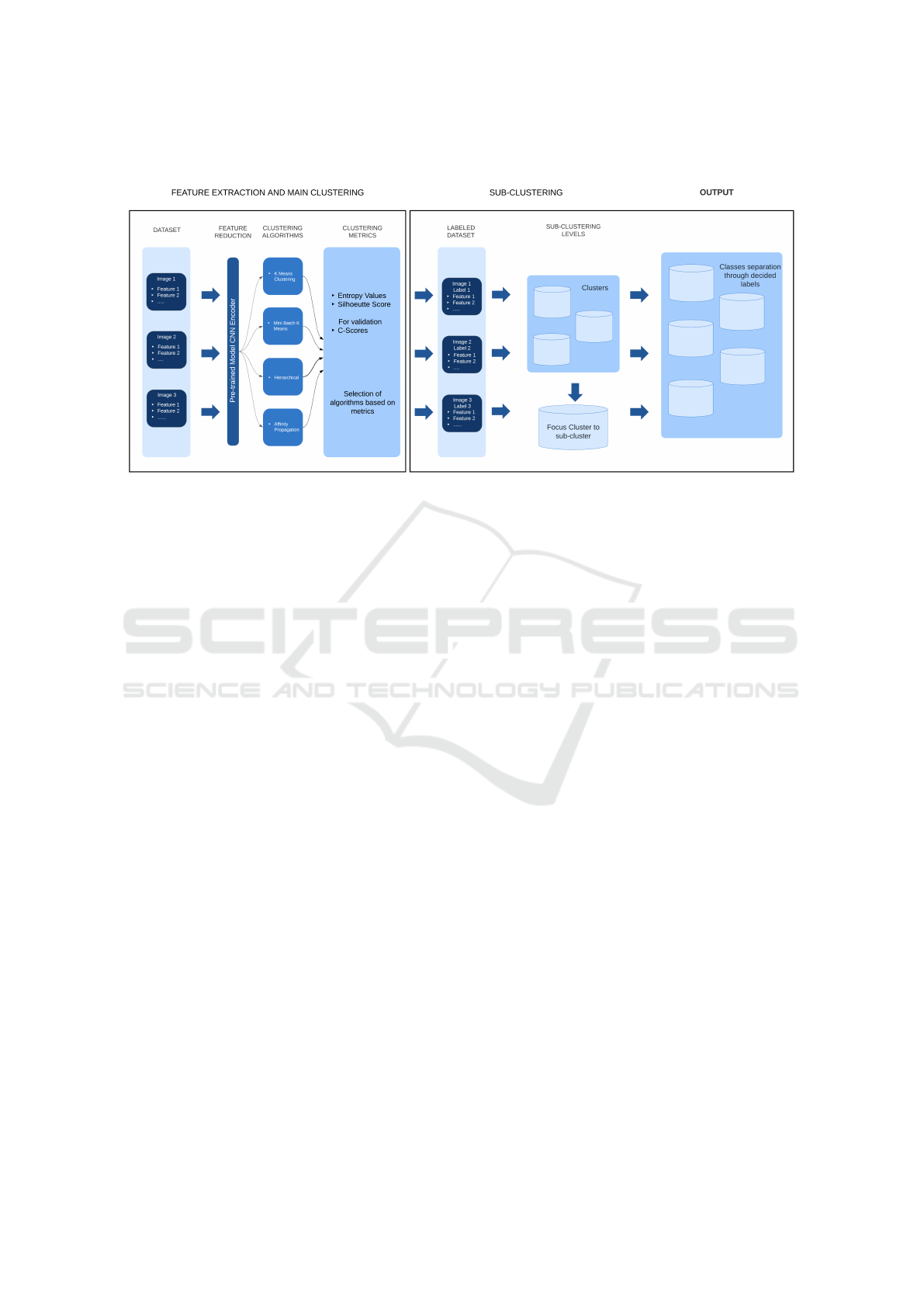
Figure 1: A Workﬂow Representation of the Proposed Methodology for Industrial Image Grouping.

reﬁne the classiﬁcation of object parts or tools for

improved precision in automated assembly lines (Fu

et al., 2024).

Similar to our work, the authors in (Biswas and Ja-

cobs, 2014) introduced a two-pronged strategy to en-

hance clustering effectiveness: Sub-clustering, where

the proposed algorithm focuses on clustering a subset

of images which aims to generate smaller but purer

clusters that provide representative examples from

each class and Active Sub-clustering, where to fur-

ther reﬁne the clustering results, the authors incor-

porate human input through an active sub-clustering

algorithm. This interaction allows for more accurate

adjustments based on user feedback, leading to im-

proved clustering outcomes. Key differences are the

use of public datasets such as face image and leaf

image datasets, along with involvement of additional

cost functions that are implemented to improve clus-

ter purities that is absent from our study. A major dif-

ference is the evaluation metric, which similar to our

work, is based on Jaccard’s co-efﬁcient. However, in

this case, the metric calculation is very different from

the one proposed later in Section 3.3.1.

2.4 Research Gap and Novel

Contributions

Despite the success of clustering techniques in indus-

trial image data analysis, several challenges remain.

One major gap in the literature is the limited use of

real-time clustering in industrial settings, particularly

for streaming image data collected from production

lines. Industrial environments often require continu-

ous monitoring and analysis of images, but traditional

clustering approaches are batch-oriented and lack the

ability to update cluster memberships dynamically as

new data arrives. Research into streaming clustering

algorithms for image data, which can handle continu-

ous data ﬂow while maintaining performance, is still

in its infancy (Wang et al., 2023).

Additionally, current methods of clustering indus-

trial images tend to rely heavily on pre-deﬁned fea-

tures or manual tuning of hyperparameters. For in-

stance, the performance of k-means or GMMs can be

sensitive to initialization and the selection of cluster

numbers. While CNN-based feature extraction has

alleviated some of these issues, the automatic deter-

mination of optimal cluster numbers for large-scale

image datasets remains an open problem. Further re-

search is needed into adaptive clustering techniques

that can dynamically adjust cluster numbers based on

data complexity, which would be particularly useful

in scenarios where the characteristics of image data

evolve over time.

Lastly, while sub-clustering approaches have

proven useful, there is a lack of standardization in

deﬁning when and how sub-clustering should be ap-

plied. Current sub-clustering techniques are often

domain-speciﬁc, and there is little research into gen-

eralizable frameworks that can be applied across dif-

ferent industrial image datasets. The development of

new metrics, such as the C-Score, which aggregates

similarities between true labels and predicted clusters,

offers a promising direction for evaluating clustering

performance, particularly when sub-clusters are in-

volved. A focus on more robust evaluation metrics

and automated sub-clustering frameworks could ﬁll

an important gap in the literature.

ICAART 2025 - 17th International Conference on Agents and Artiﬁcial Intelligence

498

3 METHODOLOGY

Given the increasing volume of image data from in-

dustrial environments, a widely-used unsupervised

approach that minimizes the reliance on expert knowl-

edge for image differentiation has not been thor-

oughly explored. Therefore, the methodology pre-

sented here utilizes available tools from the AI do-

main to introduce a degree of distinction when pro-

cessing acquired images (see Figure 1). However,

to draw a sense of rationality in introducing sub-

clustering, there must be some intermediate labeling

or distinction among images before clustering. This

can not only improve the separation process, but also

evaluate clustering at every level so as not to pursue

irrelevant or redundant approaches. We term this in-

termediate labeling as near-labels so as to provide a

baseline for separation. This is broadly explained in

Section 3.3.1.

3.1 Feature Reduction Through

Pre-Trained CNN Encoders

Using pre-trained CNN encoders for feature extrac-

tion involves repurposing convolutional layers from

models like ResNet, VGG, or EfﬁcientNet, which

were trained on large datasets such as ImageNet.

These CNNs learn a hierarchical representation of

features, where early layers capture basic patterns like

edges and textures, and deeper layers represent more

abstract patterns such as object parts. To extract fea-

tures, the output from the penultimate layer of the

CNN is commonly used. This layer, typically just

before the ﬁnal classiﬁcation layer, provides a con-

densed high-dimensional representation of the input

image. In many architectures, this corresponds to the

”global average pooling” (GAP) layer, which pools

spatial information to form a feature vector. These

feature vectors are then used as inputs to other mod-

els or classiﬁers for further processing. The following

models are used here for feature extraction:

• EfﬁcientNet-B7. A highly efﬁcient model that

uses compound scaling to optimize depth, width,

and resolution for improved performance on im-

age classiﬁcation tasks.

• InceptionV3. An advanced CNN architecture

that employs inception modules to capture multi-

scale features through parallel convolutional ﬁl-

ters, enhancing classiﬁcation accuracy.

• ResNet50. A deep residual network that intro-

duces skip connections to mitigate the vanishing

gradient problem, allowing for the training of very

deep networks with improved accuracy.

• VGG16. A straightforward and deep architecture

characterized by its use of small (3x3) convolu-

tional ﬁlters and a uniform architecture, which

signiﬁcantly impacted image classiﬁcation tasks.

The features extracted from these are fed to the

next step in the pipeline, namely the conventional

clustering algorithms. The selection of these mod-

els as backbone feature extractors is driven by their

high performance on ImageNet and diverse architec-

tural designs, leading to varied feature sets. VGG16

provides hierarchical feature maps through sequen-

tial convolutional layers, making it a robust general-

purpose extractor (Simonyan and Zisserman, 2015).

ResNet50, with its residual connections, allows for

deeper networks and improved feature discrimination,

addressing the vanishing gradient problem (He et al.,

2016). EfﬁcientNetB7 achieves superior accuracy

and efﬁciency through compound scaling of depth,

width, and resolution (Tan and Le, 2019). Incep-

tionV3 enhances multi-scale feature extraction via in-

ception modules, enabling versatility in capturing de-

tails at various resolutions, suitable for sub-clustering

tasks (Szegedy et al., 2016). Additionally, other mod-

els replicating or extending these architectures, such

as deeper variants of ResNet or scaled versions of

EfﬁcientNet, can also be considered for similar pur-

poses, given their alignment with the structural prin-

ciples and performance metrics of the selected back-

bones.

3.2 Conventional Clustering Approach

The authors implemented part of the methodology as

used in (Mathias et al., 2019), speciﬁcally different

clustering algorithms evaluated by entropy minimiza-

tion and silhouette score maximization across a range

of clusters, to determine the best algorithm and num-

ber of clusters for sub-clustering.

3.2.1 Algorithms

The following common clustering techniques were

used for a comparative analysis:

• K-Means

• Agglomerative (Hierarchical)

• Mini Batch K-Means

• Spectral Clustering

• Gaussian Mixture Model

The in-depth working of these algorithms is dis-

cussed in (Xu and Tian, 2015). These algorithms re-

quire the number of clusters to be fed as an input.

Each algorithm is fed the reduced data that is obtained

Industrial Image Grouping Through Pre-Trained CNN Encoder-Based Feature Extraction and Sub-Clustering

499

from the last layer of a CNN encoder, without any

scaling or augmentation. The results are based on the

metrics discussed in the next subsection.

3.2.2 Metrics for Selection of Clustering

Entropy Minimization. To address how many

clusters can be expected in a group of samples, the en-

tropy metric is computed for a cluster number (Math-

ias et al., 2019). It measures disorder in a vector and

is calculated as follows:

H(X) = −

n−1

∑

i=0

P(x

)log

(P(x

)) (1)

where X = x

is a label vector containing n unique

labels. P(x

) is a probability measure for every x

oc-

curring in X, calculated by

P(x

) =

no. of occurrences of x

length of X

A higher entropy value indicates more disorder in

the vector and hence, minimization is seen as a good

measure to determine the number of clusters for anal-

ysis. Once an ideal range is identiﬁed, the clustering

techniques are applied to the data for each number in

the range.

Silhouette Score. This score evaluates the similar-

ity of an object to its own cluster or group (Mathias

et al., 2019). It is calculated as follows:

S(x

) =

b(x

) − a(x

)

max{a(x

), b(x

)}

(2)

where b(x

) represents the smallest mean distance

of x

to all points in any other cluster except its own

and a(x

) is the mean distance between x

and all other

points in its own cluster. Silhouette Score is the av-

erage of all such S(x

) showing how tightly points are

clustered. It lies between −1 and 1, 1 denoting the

best case.

The performance of the algorithms is evaluated

using Silhouette scores with the maximum score be-

ing the best across all the algorithms and the range of

clusters.

3.3 Sub-Clustering Scenario

Once main clusters are formed in the given dataset

through appropriately selected algorithms, sub-

clustering is based on the cluster that needs more sep-

aration. Visually, this can be seen when the clus-

ters are well separated corresponding to higher sil-

houette scores and lower entropy values. However,

sub-clustering becomes necessary when the target en-

tities are contained in a particular cluster or group. To

proceed, we implement the same pipeline as in Sec-

tion 3.2. In addition to that, we also calculate an addi-

tional metric that serves the purpose of near-labeling.

This is explained in the following subsection.

3.3.1 C-Score

This is a novel metric used to evaluate the perfor-

mance of clustering algorithms by measuring the

overlap between true labels and predicted clusters. It

is deﬁned as the sum of Jaccard similarities for all

pairs of true labels C

and predicted clusters C

C-Score =

∑

i=1

∑

j=1

J(C

p j

) =

∑

i=1

∑

j=1

∩C

p j

∪C

p j

where k represents the total number of unique true

labels and m represents the total number of predicted

clusters.

The summation calculates the amount of common

points to the total number of points in the two sets

and runs over all classes available, in the true classes

as well as clusters formed, and does not the count

the equality of the number of clusters to the actual

classes. Thus, a clustering algorithm might have de-

tected more patterns than the actual known classes if

more clusters are formed during clustering. Simply

speaking, this metric measures the amount of inter-

sections among the clusters from two different clus-

terings or groupings. It does not necessarily represent

similarity or closeness of clusters, since the computa-

tion can exceed to higher numbers depending on the

intersections. Higher C-Score implies good amount

of intersections, for example, a defect class contained

in a cluster. The ’convergence’ alludes to the possibil-

ity that as more clusters are formed, a targeted class

may coincide with one of the clusters.

In the case of converged clustering, where each

predicted cluster contains exactly one true label and

no points from other labels, the points of each true

label C

are distributed across multiple disjoint clus-

ters C

p j

, .. . , with each cluster containing only

points from C

. For each pair where C

p j

contains

points from C

, we have:

∩C

p j

∪C

p j

∩C

p j

(3)

Since the clusters are disjoint and cover all points

in C

, the sum of these ratios for a true label C

be-

comes:

∑

∩C

p j

= 1 (4)

ICAART 2025 - 17th International Conference on Agents and Artiﬁcial Intelligence

500

Repeating this for all true labels C

, the total C-Score

is:

C-Score =

∑

i=1

1 = k (5)

Thus, under converged clustering, the C-Score

converges to k, the total number of true labels. The

equation for C-Score is symmetric with respect to k

and m, so in effect, the C-Score converges to the min-

imum of the two numbers in case of converged clus-

tering, i.e. we can say that generally,

0 < C-Score ≤ min{k, m} (6)

To provide a balanced and interpretable evaluation

of clustering performance, the C-Score is normalized

by the product of k and m:

Normalized C-Score =

C-Score

k × m

This normalization yields a metric that ranges

from 0 to 1, where a score of 1 indicates perfect

clustering alignment between the true labels and pre-

dicted clusters. By dividing the C-Score by k ×m, the

normalized C-Score accounts for both the number of

true labels and clusters, facilitating meaningful com-

parisons across different datasets and clustering solu-

tions. This approach ensures that the evaluation met-

ric is sensitive to both the richness of the true label

space and the granularity of the clustering outcome.

Hence, after normalization, the limits for converged

clustering would be

0 < Normalized C-Score ≤ min





(7)

Since for every execution, the number of clusters

are varying, it is impractical to consider only the max-

imum C-Score. Hence, after obtaining the normalized

C-Score, it is subtracted from its upper limit to cal-

culate the Convergence Difference. This difference,

referred to as the C-Score Convergence Difference,

is minimized to determine the optimal algorithm and

number of clusters going forward.

3.4 Post-Clustering Layer Alternatives

Incorporating a post-clustering layer into the method-

ology introduces an additional stage of analysis that

can reﬁne the results obtained from the initial cluster-

ing process. This layer can utilize classiﬁcation algo-

rithms, such as support vector machines (SVM), deci-

sion trees, or neural networks, to assign speciﬁc labels

or categories to the clusters formed in the preceding

step. Alternatively, other algorithms like anomaly de-

tection, regression models, or rule-based systems can

be applied, depending on the objective of the analysis.

The purpose of this post-clustering stage is to lever-

age the inherent structure identiﬁed by the clustering

to perform a more granular classiﬁcation or to extract

further insights by combining cluster properties with

supervised learning methods. Such a hybrid approach

enhances the interpretability of clusters by associat-

ing them with known classes or patterns, enabling a

more comprehensive understanding of the data.

4 IMPLEMENTATION

4.1 Dataset Overview

The data used in this study consists of images from

the Severstal Steel images (SS) dataset (Grishin et al.,

2019). It consists of images of steel produced at the

end of a production line obtained from the popular

data science website Kaggle. Although this dataset

comprises of multiple defect classes, the authors have

combined all defect class labels as a single near-label

to evaluate the methodology outlined in this study.

For practical application to avoid high time com-

plexity, the authors chose to take 1000 images for

training. These contain almost an equal amount of

two classes, namely near-label 0 corresponding to

non-defect images and near-label 1 corresponding to

defect images. Each image consists of dimensions

256 × 1600 × 3 grey-scaled for identifying different

pixels in the images that may or may not correspond

to a fault. An example image is shown in Figure 3

where the grey-scaled image shows a visible impact

region.

4.2 Model Training

The framework is only dependent on CNN encoders

for feature extraction, whereas the training is only un-

dertaken during the clustering process. This leads to a

reduction of the run-time of the outlined framework,

thereby making it efﬁcient for inclusion in a larger

pipeline.

Post feature extraction, the clustering algorithms

are run for a ﬁxed range of clusters from 2 to 50.

For each algorithm and number of clusters, the cor-

responding metrics from Section 3.2.2 are calculated

leading to a criteria for selection. Principal Compo-

nent Analysis (PCA) is applied to the input data to

improve time complexity of applying multiple clus-

tering algorithms in a sequence. However, the PCA

is only kept to minimum of the size of the input, i.e.

either the number of samples or features.

Industrial Image Grouping Through Pre-Trained CNN Encoder-Based Feature Extraction and Sub-Clustering

501

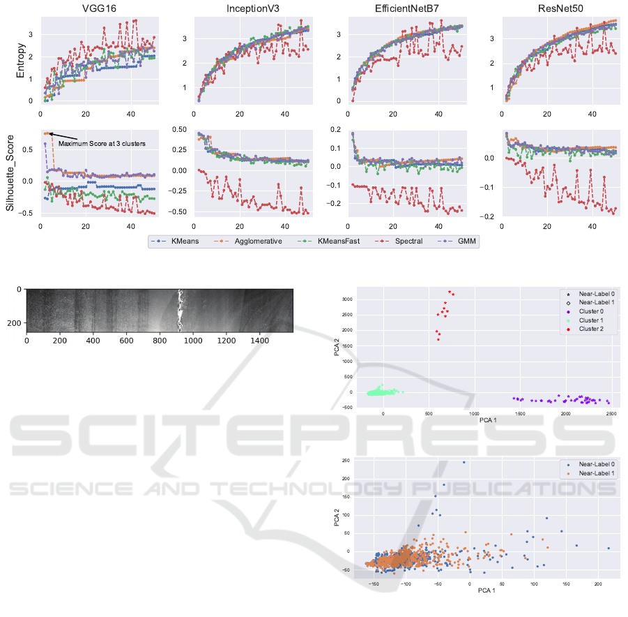
Figure 2: Entropy and Silhouette Scores for the Main Clustering on CNN Encoder-Based Data.

Figure 3: Grey-scaled Pre-processed Image from SS

Dataset.

We follow the ’Min-Max’ criteria established in

(Mathias et al., 2019) to exclude those algorithms that

exude larger entropy and minimum silhouette scores.

This leads to a range of clusters that can be contended

with for further analysis. This process is repeated

for every level of sub-clustering, however, the use of

’Min-Max’ criteria or the C-Score is subject to the

user based on the observed clusters.

5 RESULTS

The extraction of features using the CNN models rea-

sonably is the primary time-consuming step in the

proposed approach. However, it eliminates the need

for computationally intensive clustering on raw inputs

directly. Additionally, this approach avoids the com-

plexity and resource burden of designing custom fea-

ture extraction methods tailored to speciﬁc datasets.

The trade-off lies in leveraging these optimized mod-

els, whose outputs can exceed expectations by deliv-

ering robust, transferable representations that enhance

the efﬁciency and reliability of subsequent clustering

tasks. This balance between computational efﬁciency

and effective feature extraction highlights the practi-

cality of using these available models.

(a) Agglomerative Clustering of Reduced Features with 3 Clusters.

(b) Cluster 1 which contains all Near-Labels 1.

Figure 4: Main Clustering Best Performance.

5.1 Main Clustering Evaluation

The performance of the CNN encoders, evaluated

using Min-Max approach of Entropy and Silhouette

Score is presented in Figure 2 with entropy shown in

the top row and silhouette scores in the bottom row.

Entropy. For all architectures, entropy consistently

increases as the number of clusters grew, indicating

higher disorder in cluster assignments as more clus-

ters were formed. This trend was observed across

all models, reﬂecting a general increase in complexity

with additional clusters.

ICAART 2025 - 17th International Conference on Agents and Artiﬁcial Intelligence

502

Silhouette Score. The silhouette scores follow a

different pattern, peaking early and progressively de-

creasing as the number of clusters increased. For

VGG16, the maximum silhouette score is observed at

3 clusters, as indicated by the labeled point in the ﬁg-

ure. This suggests that the optimal number of clusters

for VGG16 is 3, offering the best separation and co-

hesion among clusters. Beyond 3 clusters, silhouette

scores declined for all networks, and in several cases,

the scores dropped to negative values, particularly for

the red cluster, indicating poor clustering quality.

Across all models, the initial silhouette scores in-

dicated strong clustering quality, but the drop in per-

formance as the number of clusters increased suggests

that over-clustering likely occurred, leading to less

meaningful groupings. The results show that VGG16

was the most effective at maintaining cluster quality,

with 3 clusters yielding the most optimal outcome in

terms of the silhouette score.

For the purpose of visualization, the extracted data

from VGG16 was further reduced to two components

based through PCA. Figure 4 presents the best per-

forming clustering algorithm, i.e Agglomerative on

this data. Figure 4a) shows the distinctly clustered

group of points into 3 well-distanced groups while

Figure 4b) shows the focus cluster 1 which contains

all the near-labels 1 of the original data.

5.2 Sub-Clustering Evaluation

Once the main clustering is done, the necessity of sub-

clustering is dependent on the user. In this case, we

applied the same methodology as in the main cluster-

ing. However, the evaluation at later levels is done ei-

ther using Min-Max criteria or through C-Score Con-

vergence Difference to identify which algorithm and

what number of clusters are effective in discerning the

near-labels in smaller groups. For example, after main

clustering, level 1 clustering yields the results shown

in Figure 5.

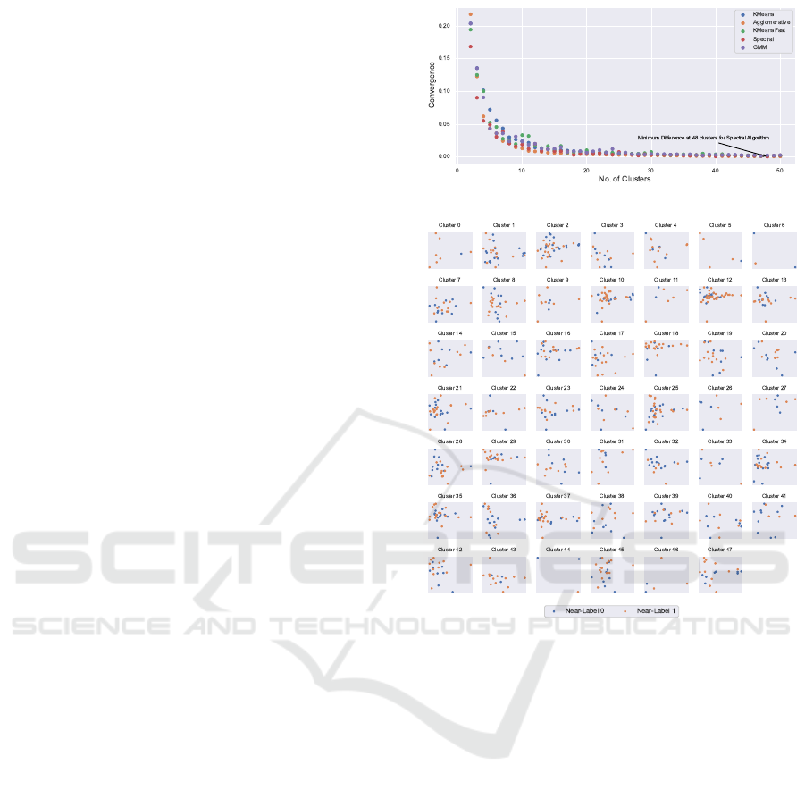
The C-Score Convergence Difference yields the

minimum value for the Spectral algorithm with 48

clusters of main cluster 1 in the previous step (see

Figure 5a)). The 48 clusters are shown in Figure 5b)

which shows some dominant groupings with respect

to near-labels. For example, clusters 0, 5, 8, 11, 22,

29, 43, and 46 mainly consist of near-label 1. Many

clusters are still visibly indistinguishable with respect

to the initial labels like clusters 2, 12, 21, 25, and

42. Since elements are grouped into small sizes, it

becomes easier to work with smaller clusters to make

a certain distinction through near-labels. For this rea-

son, cluster 25 was chosen for the next sub-clustering.

As more clusters are formed, the C-Score Con-

(a) C-Score Convergence Difference at Level 2 Clustering.

(b) Best Performing Spectral Algorithm with 48 Clusters.

Figure 5: Level 1 Clustering of Cluster 1 from Main Clus-

tering.

vergence Difference will eventually lead to the mini-

mum score of 0 as the number of clusters matches the

number of samples. In level 2 clustering, since clus-

ter 25 only had 33 points, the authors chose to only

work with 2 clusters, same as the number of near-

labels. The corresponding clusters for each algorithm

are shown in Figure 6. At this stage, the decision

to select the appropriate clusters is dependent on the

user. For example, GMM clustering for two clusters

shows that cluster 1 must be inspected deeply, since

cluster 1 mainly contains near-labels 1. However,

GMM also exihibits the best clustering since most of

near-labels 1 are entirely contained in cluster 1 while

cluster 0 has a majority of near-labels 0. Observably,

cluster 0 can be well separated further into 2 clusters

with sub-clustering imminent for cluster 1. The au-

thors have, however, chosen to halt the sub-clustering

process at this level to avoid redundancy.

Industrial Image Grouping Through Pre-Trained CNN Encoder-Based Feature Extraction and Sub-Clustering

503

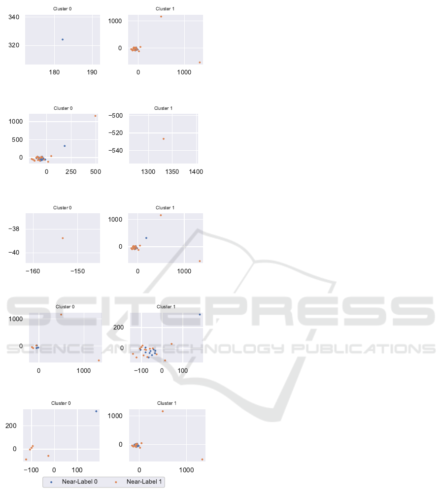
(a) KMeans Clustering.

(b) Agglomerative Clustering.

(d) Spectral Clustering.

(e) GMM Clustering.

Figure 6: Level 2 Clustering of Cluster 25 from Level 1

Clustering.

5.3 Observations

We make some observations from the employed

scheme of sub-clustering:

• In main clustering, it is evident that using just

available CNN encoders for feature extraction is

sufﬁcient in some cases to mark a certain bound-

ary between images, as in Figure 4. However, this

does not guarantee that the extraction or clustering

gives optimal results.

• The C-Score is a set-related metric, hence it can

be used to decide the similarity between collec-

tions. However, in this scenario, it is only useful

when some initial distinction is available to judge

the quality of clustering.

• In the absence of near-labels, sub-clustering is

purely visual, with only distances between sam-

ples determining cluster structures and no other

information.

• For sub-clustering, since the number of samples

is reduced, this scheme can also incorporate other

feature reduction techniques on the same data

within sub-clustering levels. This can help in im-

proving clustering. However, this has not been

implemented in this study to avoid an overload of

framework execution.

6 AN END-TO-END LABELING

SCHEME IN PRODUCTION

ENVIRONMENTS

To augment the undertaken experiment, an end-to-end

labeling scheme can be constructed using only the ba-

sic tools of machine learning, as shown in Figure 7.

In any application building, the ﬁner front-end archi-

tecture is dependent on the end-user/client. However,

on the production ﬂoor, a simple working application

that comprises of database, clustering algorithms and

neural networks is beneﬁcial for the operator to im-

mediately inspect product quality without waiting for

deeper quality inspection. The operator also beneﬁts

through clustering in identifying varying processes

from the captured images. For example, as seen in

Figure 4a), three patterns are distinctly recognized by

the algorithms with one cluster completely contain-

ing the defect labels. The other groups of points can

be further investigated for mechanical properties or

process related parameters issues.

To complete such a predictive application, an ap-

plication workﬂow that begins with capture of image,

then ﬂows through a storage such as database, passed

through a pre-trained model prediction followed by a

custom classiﬁcation to obtain groups is a fairly easy

task as long as the architecture remain in one location

such as a local PC. The complexity however increases

when the distribution of layers is across different plat-

forms such as cloud storage for data, followed by re-

mote location of analysing PC and output transmis-

sion to correct users/clients. This falls in the domain

ICAART 2025 - 17th International Conference on Agents and Artiﬁcial Intelligence

504

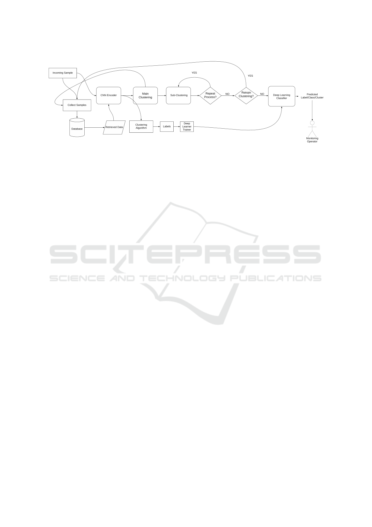
Figure 7: An End-to-End Labeling Scheme with Sub-Clustering.

of Internet-of-Things which can be investigated in fu-

ture research.

7 CONCLUSION

A labeling scheme involving a transfer learning ap-

proach utilizing available CNN encoders for feature

extraction of industrial images and transferring them

to clustering algorithms for cluster labels is presented.

The layers of the architecture can be varied accord-

ing to the user requirements, for example, replacing

CNN networks with custom nets which is an addi-

tional advantage. Similarly, the clustering algorithms

used can also be varied depending on the problem re-

quirement. The results that are presented show that

such a scheme if developed for production ﬂoors, it

can assist the monitoring operators in detecting vary-

ing patterns which are critical in avoiding defects or

anomalies. Because pre-trained models are used, it

is clear that analysis becomes more efﬁcient and ro-

bust as no customized feature extraction or advanced

knowledge of process or product is required to la-

bel/group the incoming samples. The applicability of

this approach can also be considered to be very broad

since images are fed directly into the feature extrac-

tion steps without any pre-requisite condition of their

origin. An outlook on the development of a working

application on the production ﬂoor is also discussed.

The focus in this study is not improvement of pro-

posed methodology, rather the practical application in

real-time scenarios. Improvement of clustering algo-

rithms can be further undertaken in a deeper studies

involving multiple datasets, varied CNN models and

comparisons with established baselines. Some topics

related to cluster convergence through C-Score and

cluster proﬁling of image-based data can be investi-

gated in future works.

REFERENCES

Biswas, A. and Jacobs, D. (2014). Active subclustering.

Computer Vision and Image Understanding, 125:72–

84.

Cardoso, D. and Ferreira, L. (2021). Application of predic-

tive maintenance concepts using artiﬁcial intelligence

tools. Applied Sciences, 11(1).

Chang, J., Wang, L., Meng, G., Xiang, S., and Pan, C.

(2017). Deep adaptive image clustering. In 2017 IEEE

International Conference on Computer Vision (ICCV),

pages 5880–5888.

Dalal, N. and Triggs, B. (2005). Histograms of oriented gra-

dients for human detection. In 2005 IEEE Computer

Society Conference on Computer Vision and Pattern

Recognition (CVPR’05), volume 1, pages 886–893

vol. 1.

Daugman, J. G. (1985). Uncertainty relation for resolution

in space, spatial frequency, and orientation optimized

by two-dimensional visual cortical ﬁlters. J Opt Soc

Am A, 2(7):1160–1169.

Fan, C.-L. (2024). Multiscale feature extraction by using

convolutional neural network: Extraction of objects

from multiresolution images of urban areas. ISPRS

International Journal of Geo-Information, 13(1).

Fu, K., Dang, X., Zhang, Q., and Peng, J. (2024). Fast

uois: Unseen object instance segmentation with adap-

tive clustering for industrial robotic grasping. Actua-

tors, 13(8).

Grishin, A., V, B., iBardintsev, inversion, and Oleg (2019).

Severstal: Steel defect detection.

Hartner, R., Komar, J., and Mezhuyev, V. (2022). An ap-

proach for increasing the throughput of a cnn-based

industrial quality inspections system with constrained

devices. In Proceedings of the 2022 11th International

Conference on Software and Computer Applications,

ICSCA ’22, page 179–184, New York, NY, USA. As-

sociation for Computing Machinery.

He, K., Zhang, X., Ren, S., and Sun, J. (2016). Deep resid-

ual learning for image recognition. In 2016 IEEE Con-

ference on Computer Vision and Pattern Recognition

(CVPR), pages 770–778.

Industrial Image Grouping Through Pre-Trained CNN Encoder-Based Feature Extraction and Sub-Clustering

505

Li, W., Hannig, J., and Mukherjee, S. (2021). Subspace

clustering through sub-clusters. Journal of Machine

Learning Research, 22(53):1–37.

Lowe, D. G. (2004). Distinctive image features from scale-

invariant keypoints. International Journal of Com-

puter Vision, 60(2):91–110.

Mathias, S. G., Großmann, D., and Sequeira, G. J. (2019). A

comparison of clustering measures on raw signals of

welding production data. In 2019 International Con-

ference on Deep Learning and Machine Learning in

Emerging Applications (Deep-ML), pages 55–60.

Oyelade, J., Isewon, I., Oladipupo, O., Emebo, O.,

Omogbadegun, Z., Aromolaran, O., Uwoghiren, E.,

Olaniyan, D., and Olawole, O. (2019). Data cluster-

ing: Algorithms and its applications. In 2019 19th

International Conference on Computational Science

and Its Applications (ICCSA), pages 71–81.

Saad, N., Sabri, N. M., Hasan, A., Ali, A., and Saleh, H. M.

(2015). Defect segmentation of semiconductor wafer

image using k-means clustering. In Design and Devel-

opment of Sustainable Manufacturing Systems, vol-

ume 815 of Applied Mechanics and Materials, pages

374–379. Trans Tech Publications Ltd.

Silva, W. and Capretz, M. (2019). Assets predictive main-

tenance using convolutional neural networks. In 2019

20th IEEE/ACIS International Conference on Soft-

ware Engineering, Artiﬁcial Intelligence, Networking

and Parallel/Distributed Computing (SNPD), pages

59–66.

Simonyan, K. and Zisserman, A. (2015). Very deep con-

volutional networks for large-scale image recognition.

In Bengio, Y. and LeCun, Y., editors, 3rd Interna-

tional Conference on Learning Representations, ICLR

2015, San Diego, CA, USA, May 7-9, 2015, Confer-

ence Track Proceedings.

Strang, G. and Nguyen, T. (1996). Wavelets and Filter

Banks. Wellesley-Cambridge Press, Philadelphia, PA.

Szegedy, C., Vanhoucke, V., Ioffe, S., Shlens, J., and Wojna,

Z. (2016). Rethinking the inception architecture for

computer vision. In 2016 IEEE Conference on Com-

puter Vision and Pattern Recognition (CVPR), pages

2818–2826.

Tan, M. and Le, Q. (2019). EfﬁcientNet: Rethinking model

scaling for convolutional neural networks. In Chaud-

huri, K. and Salakhutdinov, R., editors, Proceedings of

the 36th International Conference on Machine Learn-

ing, volume 97 of Proceedings of Machine Learning

Research, pages 6105–6114. PMLR.

van der Maaten, L. and Hinton, G. (2008). Visualizing data

using t-sne. Journal of Machine Learning Research,

9(86):2579–2605.

Wang, X., Wang, Z., Wu, Z., Zhang, S., Shi, X., and Lu, L.

(2023). Data stream clustering: An in-depth empirical

study. Proc. ACM Manag. Data, 1(2).

Xie, J., Girshick, R., and Farhadi, A. (2016). Unsuper-

vised deep embedding for clustering analysis. In Bal-

can, M. F. and Weinberger, K. Q., editors, Proceed-

ings of The 33rd International Conference on Ma-

chine Learning, volume 48 of Proceedings of Machine

Learning Research, pages 478–487, New York, New

York, USA. PMLR.

Xu, D. and Tian, Y. (2015). A comprehensive survey

of clustering algorithms. Annals of Data Science,

2(2):165–193.

Xu, R. and Wunsch, D. (2005). Survey of clustering al-

gorithms. IEEE Transactions on Neural Networks,

16(3):645–678.

Zhang, Q. and Chen, J. (2022). Distributed learning of ﬁ-

nite gaussian mixtures. Journal of Machine Learning

Research, 23(99):1–40.

ICAART 2025 - 17th International Conference on Agents and Artiﬁcial Intelligence

506