
Formation Analysis for a Fleet of Drones: A Mathematical Framework
Emiliano Traversi
1
, Michal Barcis
2
, Lorenzo Bellone
2
, Agata Barcis
2
, Dina Ahmim-Bonaldi
2
,
Eliseo Ferrante
3
and Enrico Natalizio
2
1
IDO Department, ESSEC Business School, Cergy-Pontoise, France
2
Technology Innovation Institute, Abu Dhabi, U.A.E.
3
New York University Abu Dhabi, Abu Dhabi, U.A.E.
Keywords:
Robot and Multi-Robot Systems, Task Planning and Execution, Formation Study.
Abstract:
We consider a dynamic coverage scenario, where a group of agents (e.g., Unmanned Aerial Vehicles (UAVs))
is exploring an environment in search of a moving target (e.g., survivors on a lifeboat). We assume UAVs are
capable to achieve, maintain, and move in formation (e.g., to maintain connectivity). This paper addresses
the question “Which formation maximizes the chance of finding the target?”. We propose a mathematical
framework to answer this question. The proposed framework is generic and can be easily applied to various
formations and missions. We show how the framework can identify which formation will result in better
performance in the type of missions we consider. We analyze how different factors, namely the target speed
relative to the group, affect the performance of the formations. We validate the framework against simulations
of the considered scenarios. The supplementary video material including the real-world implementation is
available at https://youtu.be/ mYmTnAJi-I?si=dSmVVNZOjj5NbSG1.
1 INTRODUCTION
Groups of agents or robots can be advantageous over
single agents in several applications. Search missions
(looking for survivors or faults or oil spills, etc.) con-
stitute important applications and are also the sub-
ject of active research (Ivi
´
c et al., 2020). Deploy-
ing groups of searching agents can increase the ef-
ficacy and efficiency in such missions. An important
decision is how to divide the search among agents.
A possible choice is to divide the area into partitions
and assign agents to independently explore them (Liu
et al., 2023; Mazdin et al., 2020; Kovacina et al.,
2002). In other situations, it may be advantageous to
deploy search parties consisting of multiple agents to
explore a common large area. For example, searching
in groups can be advantageous when diverse capabil-
ities are available within each search party (Dorigo
et al., 2013). For autonomous (unmanned) search-
ing agents, the need to travel in search parties is mo-
tivated by limited access to long-range communica-
tion devices: For instance, only some robots may
be equipped with satellite modems allowing commu-
nication with the mission control station, while all
robots are equipped with shorter range transceivers.
Agents employed in group search must travel in
close proximity, but the exact relative positions of the
agents vary. The specific choice of the set of relative
positions of the agents can be referred to as a forma-
tion. Agents operating in formations present advan-
tages: For instance, birds fly in specific formations
to save energy (Bajec and Heppner, 2009), which in-
spired the development of systems that can reduce
fuel consumption in aircrafts (Afonso et al., 2023;
Antczak et al., 2022; Hartjes et al., 2019). Formation
flights can also be used in the decentralized handling
of control tasks for surveillance to optimize a system
with respect to cost and weight constraints (Anderson
et al., 2008). Formation control – the study on how to
achieve and maintain a formation – is an active field of
research (Justh and Krishnaprasad, 2002; Wang et al.,
2007; Paul et al., 2008; Chao et al., 2012). The focus
of our work is not on formation control. We instead
assume a reliable method for formation control is al-
ready available.
The main hypothesis in this work is that some for-
mations are better than others in group search mis-
sions, depending on the mission profile. We propose
a mathematical model that can analyze how differ-
ent choices of formation influence the target detec-
tion chance. We consider the dynamic coverage (Pa-
patheodorou and Tzes, 2018; Atınc¸ et al., 2020), or
sweeping coverage (Cheng and Savkin, 2009; Zhai
and Hong, 2012; Zhai and Hong, 2013; Saska et al.,
2013) problem. To the best of our knowledge, we fo-
cus on the first time the effect of specific formation
Traversi, E., Barcis, M., Bellone, L., Barcis, A., Ahmim-Bonaldi, D., Ferrante, E. and Natalizio, E.
Formation Analysis for a Fleet of Drones: A Mathematical Framework.
DOI: 10.5220/0013189400003890
In Proceedings of the 17th International Conference on Agents and Artificial Intelligence (ICAART 2025) - Volume 1, pages 471-480
ISBN: 978-989-758-737-5; ISSN: 2184-433X
Copyright © 2025 by Paper published under CC license (CC BY-NC-ND 4.0)
471
for intercepting a moving target.
The pursuer-evader task is related to the one con-
sidered in this paper (Hespanha et al., 1999). In (Yu
et al., 2019; de Souza et al., 2021), multiple pursuers
have been used to maximize their chances. In (Wei
and Yanq, 2018), pursuers are used to lure the evader
into their paths, while others simultaneously establish
an encirclement to capture the target. In the above
work, the pursuers’ remain close to the evader, rather
than finding it in an unknown environment.
In contrast to the above literature, this paper
presents a different approach to dynamic coverage,
focusing on the analysis of the use of different for-
mations to search for a moving target with an un-
known trajectory. The main contribution of this work
is a mathematical framework for this analysis (Sec-
tion 3). We validate the correctness of the framework
in a simulated mission with Unmanned Aerial Vehi-
cles (UAVs), and show a proof of concept with real
UAVs (Section 4) where the framework can be use-
ful. We conclude the paper in (Section 5).
2 PROBLEM STATEMENT
We consider a search mission in which a group of
robots in formation has to find a moving target. We
introduce a mathematical framework that models the
effect of the formation on the search task. To sim-
plify the mathematical treatment, we consider arbi-
trary linear search trajectories followed by the group
of agents. We assume these are planned in a way to
cover the parts of the environment where the target
may appear. Each sweeping trajectory is modeled as
a straight corridor depicted vertically: the agents tra-
verse it from bottom to top. Let n
d
be the number
of agents. Each agent is modeled as a rectangular
area with size ℓ
h
× ℓ
v
that represents the agent field
of view. If agents correspond to UAVs, the rectan-
gular area represents the field of view of the camera
equipped on the drone. The agents move within the
corridor without changing their relative positions and
at a constant speed of v
d
. We assume a reference sys-
tem that is fixed and centered on the group (in other
words, the group does not move with respect to the
considered reference frame). Figure 1 shows an illus-
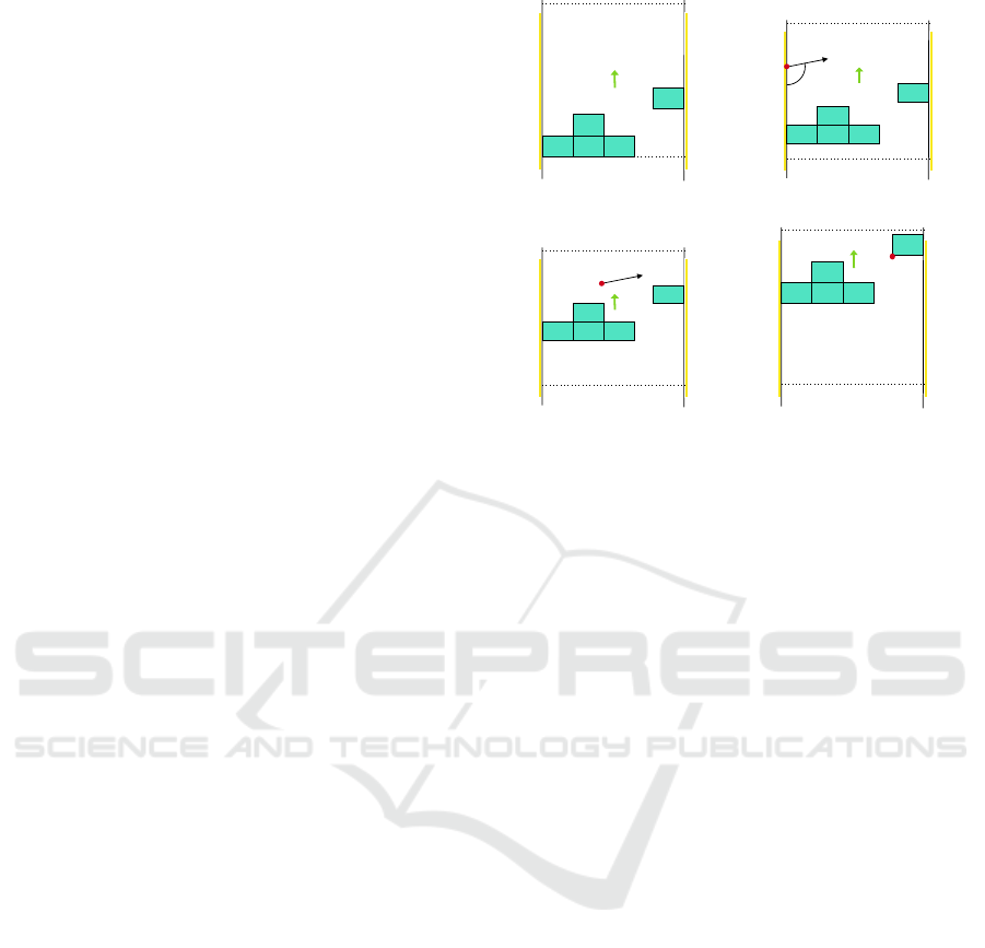
trative example.
We introduce: The maximum and minimum entry
points of the target, x
min
t
and x
max
t
; The starting and
ending points of agent exploration, x
min
d
and x
max
d
.
The agent group has to detect the presence of a
moving target within the corridor. The mission be-
gins with the agents group positioned at the point x
min
d
(lower dotted horizontal lines in Figure 1), and it tra-
x
min
d
x
max
d
x
max
t
x
min
t
v
d
(a) Start of the exploration.
x
min
d
x
max
d
x
max
t
x
min
t
v
d
v
t
θ
(b) Target’s appearance.
x
min
d
x
max
d
x
max
t
x
min
t
v
d
v
t
(c) Target follows trajectory.
x
min
d
x
max
d
x
max
t
x
min
t
v
d
(d) Target is intercepted.
Figure 1: Example of a successful exploration.
verses the corridor at a constant speed v
d
up to the
point x
max
d
(upper dotted horizontal lines in Figure 1).
We assume that at any moment during the exploration,
a target (represented as a red dot in Figure 1) enters
the corridor from one of its edges at a randomly gen-
erated point within the interval [x
min
t
,x
max
t
] (see the
yellow left border in Figure 1) and with a random
orientation (distributed in the range [0,π]), constant
speed v
t
, and following a straight trajectory. We indi-
cate with P
T
(x) the probability that the target shows
up at a given position x ∈ [x
min
t
,x
max
t
].
During the exploration, if the target enters any of
the agent’s rectangular area, it is considered inter-
cepted. If instead the target exits the other side of the
corridor without entering any rectangle, it is consid-
ered missed. Furthermore, exploration stops when all
agents have crossed the maximum exploration point,
x
max
d
. If the target has not been intercepted by that
time, it is considered missed.
3 MODEL DEFINITION
In this section, we present the framework enables to
compute the probability for a given group formation
to intercept a target (hereby referred to as the inter-
ception probability) in a mission with a customizable
profile.
ICAART 2025 - 17th International Conference on Agents and Artificial Intelligence
472
3.1 Framework Overview
Let x represent the distance between the target’s entry
point and the group of agents
1
. Define S as the set of
all subsegments of [0,π], and S as the set of all sub-
sets of S (i.e., S is the power set of S). Key to our
analysis is representing the set of interceptable direc-
tions S
x
⊆ S , that is the set of maximal (with respect
to inclusion) segments that correspond to values of θ
that lead to interception.
S
x
x
Figure 2: Example of S
x
for a specific formation.
Figure 2 provides an example of S
x
for a specific
formation and distance x between the formation and
the target entry point (in red). Here, S
x
contains the
two segments in purple.
Let P
x
(θ) be the probability that, for an entry point
x, the direction of the target is equal to θ and let P
x
be
the probability that the target is intercepted if it enters
at a distance x from the formation of agents. We can
compute P
x
as:
P
x
=
∑
[θ
1
,θ
2
]∈S
x
Z
θ
2
θ
1
P
x
(θ)dθ (1)
In this equation, only entrance angles that belong to
S
x
and that yield to interceptions are integrated. Con-
sider the case where all entry angles are equally prob-
able (P
x
(θ) =
1
π
, ∀θ ∈ [0,π]). In this case, P
x
(denoted
as P
x
) is:
P
x
=
∑
[θ
1
,θ
2
]∈S
x
Z
θ
2
θ
1
1
π
· dθ =
1
π
∑
[θ
1
,θ
2
]∈S
x
(θ
2
− θ
1
) .
(2)
In the rest of the paper we will focus only on this case.
3.2 Modeling Formations
The type of formation selected impacts significantly
the complexity of the description of the set S
x
. In this
1
In this paper we will denote by x a position on the ver-
tical axis. Depending on the context, it may indicate the
target entry point or the position of the formation.
work, we focus on formations that allow the set S
x
to
have the following properties:
• Symmetry. S
x
is symmetric if its value does not
depend on the entry side of the target but only on
the distance x. This property allows us to assume,
without loss of generality, that the target enters
from only one of the two sides.
• Scalar-representability. S
x
is scalar-representable
if it consists of one single segment of the form
[0,θ
x
]. Loosely speaking, this holds when forma-
tions do not have “holes” in the range of angles
θ that lead to interception. This property allows
us to see S
x
as a function S
x
: R → [0, π] that for
each entry point x returns the maximal entry angle
θ
x
that leads to an interception. The entry point x
is to be understood as an absolute value, so the
above holds regardless of whether the target en-
ters in front or behind the formation.
Working with a set of interceptable directions that
is symmetric and scalar-representable allows us to
have a more tractable mathematical model. Having
said this, the framework is general enough to be ex-
tendable also to the cases where “holes” are present.
Figure 3: Formations considered.
Among the formations that meet the above proper-
ties, we study the three of them: line, arrow, and vee
formations (see Fig. 3). We conclude by noting that
the choice of the formation is not the only factor that
can affect whether the set S
x
is scalar representable or
not, as it will become clear in the next section. Thus,
conditions on the formation are necessary but not suf-
ficient for having a scalar-representable set of inter-
ceptable directions.
3.3 Calculating P
x
Except when explicitly stated, in the rest of this doc-
ument we assume a set of interceptable directions S
x
that is symmetric and scalar-representable. To make
the analysis easier to tackle, we represent S
x
as a com-
position of two functions, f
D
(θ) and f
S
(x):
S
x
= [0, f
D
( f
S
(x))] (3)
The function f
S
(x) : R → [0,π] (where the “S”
stands for static) calculates the maximal entry angle at
which we have an intersection between the target and
the group of agents in a given formation, for a given
snapshot of the mission whereby the agents do not
Formation Analysis for a Fleet of Drones: A Mathematical Framework
473
move (i.e., v
d
= 0). This function takes into account
the contribution of the specific formation but does not
consider the magnitude of the speed of the target v
t
since agents are considered static (v
d
= 0). The func-
tion f
D
(x) : [0, π] → [0,π] (where the “D” stands for
dynamic) models how the speed of the target v
t
and
the speed of the agents v
d
modify the maximal entry
angle calculated with f
S
(x).
Eq. (3) allows to simplify the computation of P
x
(see Eq. (2)):
P
x
=
1
π
∑
[θ
1
,θ
2
]∈S
x
(θ
2
− θ
1
) =
f
D
( f
S
(x))
π
. (4)
Eq. (4) shows that, if all target entry angles are equally
probable, it is sufficient to determine the maximum
entry angle for the given entry point and divide it by
π to obtain the probability of interception.
In the following, we detail how to calculate f
D
(θ)
and f
S
(x) for specific scenarios, as a guideline for ap-
plying the framework to any scenario with symmetric
and scalar-representable S
x
.
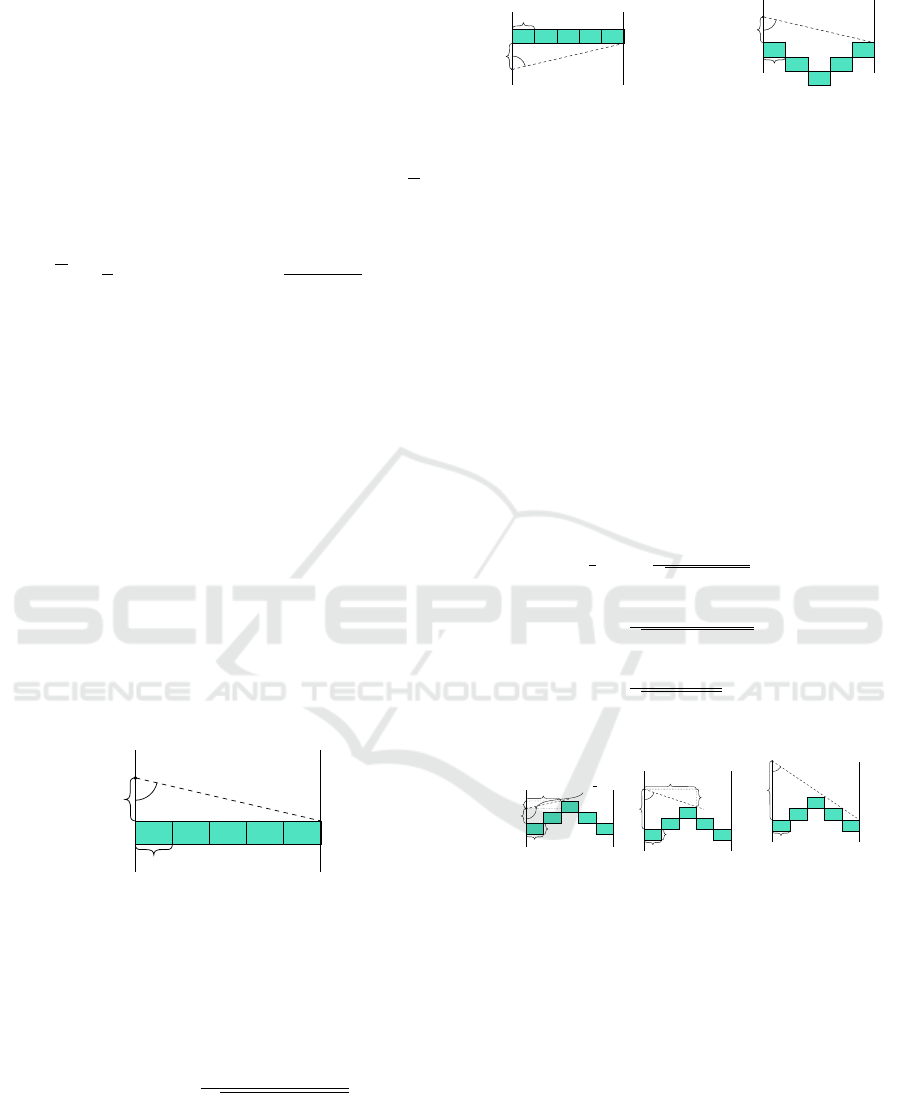
3.3.1 Calculation of f
S
(x)
We formalize the value of f
S
(x) as a function of the
entry point of the target. According to the formation
used, the definition will differ and incorporate the pa-
rameters ℓ
h
, ℓ
v
, and the size of the group n
d
. For sim-
plicity, we assume that we only consider an odd num-
ber of agents n
d
and we introduce k that identifies the
“‘depth” of the formation k = (n
d
− 1)/2.
θ
x
ℓ
h
Figure 4: How to compute f
L
S
(x) for a line formation.
Line-Formation. The function f
S
(x) applied to a
line formation is denoted as f
L
S
(x). Figure 4 shows
how to calculate f
L
S
(x) by applying the definition of
sine to the right triangle with vertices in the target en-
try point and in two extreme points of the formation:
f
L
S
(x) = arcsin
(2k + 1)ℓ
h
q
(2k + 1)
2
ℓ
2
h
+ x
2
(5)
If the reference system is defined appropriately,
Eq. (5) can also be used for computing f
S
(x) when
the target enters from the back of a line formation, in
front of a vee-formation or from the back of an arrow-
formation (see Fig. 5 for some examples).
θ
x
ℓ
h
(a) Target enter-
ing in the back of
a line formation.
θ
x
ℓ
h
(b) Target enter-
ing in the front of
a vee formation.
Figure 5: When to apply f
L
S
(x) to other configurations.
Vee and Arrow Formations. In this paragraph, we
describe f
S
for a target entering in the front of an ar-
row formation and in the back of a vee formation, us-
ing the same equation thanks to symmetry. We denote
it as f
AV
S
in both cases.
The more complex nature of the arrow and vee for-
mations makes it necessary to split the analysis into
three cases, depending on where the target hits the
formation when it has a direction corresponding to its
maximal entry angle: (1) The nearest side of the ar-
row (if 0 ≤ x ≤ kℓ
v
, see Figure 6a); (2) The “head” of
the arrow (if kℓ
v
≤ x ≤ (2k + 1)ℓ
v
, see Figure 6b); (3)
The farthest side of the arrow (if x ≥ (2k + 1)ℓ
v
, see
Figure 6c):
f
AV
S
(x) =
π
2
+ arcsin
kℓ
v
− x
q
(kℓ
v
− x)
2
+ k
2
ℓ
2
h
0 ≤ x ≤ kℓ
v
arcsin
(k + 1)ℓ
h
q
(k + 1)
2
ℓ
2
h
+ (x − kℓ
v
)
2
kℓ
v
≤ x ≤ (2k + 1)ℓ
v
arcsin
(2k + 1)ℓ
h
q
(2k + 1)
2
ℓ
2
h
+ x
2
(2k + 1)ℓ
v
≤ x
(6)
θ
x
ℓ
h
θ −
π
2
ℓ
v
kℓ
v
− x
kℓ
h
(a) Target touching the
nearest side of the arrow.
θ
x
ℓ
h
ℓ
v
x − kℓ
v
(k + 1)ℓ
h
(b) Target touching
the head of the arrow.
θ
x
ℓ
h
(c) Target touching
the farthest side of the
arrow.
Figure 6: f
AV
S
(x) for different target entry points.
3.3.2 Calculation of f
D
(x)
f
D
does not depend on the formation because it mod-
els how the maximum entry angle obtained in the
static case is altered when the agents have a veloc-
ity greater than zero. Instead, f
D
depends on the entry
point of the target. In the following, we indicate with
f
F
D
(θ) and f
B
D
(θ) the values of f
D
when the target en-
ters from the front or from the back.
If the agents are in motion, it becomes necessary
to employ a formula that indicates how the speed of
the target is perceived by the moving agents (recall
ICAART 2025 - 17th International Conference on Agents and Artificial Intelligence
474
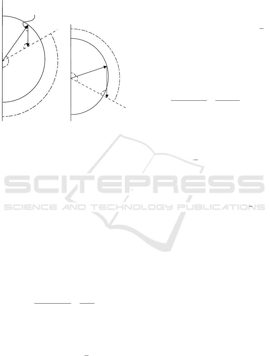
v
d
v
t
= 1
θ
f
F
D
(θ)
π − f
F
D
(θ)
θ
(a) Computation of f
F
D
(θ)
if the target enters in front
of the agents.
v
d
v
t
= 1
θ
f
B
D
(θ)
θ − f
B
D
(θ)
π − f
B
D
(θ)
(b) Computation of f
B
D
(θ)
if the target enters behind
the agents
Figure 7: Computation of f
F
D
(θ) and f
B
D
(θ).
the reference system is fixed with the agent group).
We observe that, when the target enters in front of the
agents, moving agents increase the chances of inter-
cepting the target, which corresponds to an increased
maximum entry angle in the dynamic case. Similarly,
when the target enters from the rear of the forma-
tion, the maximum entry angle also increases in the
dynamic case.
The formulas for f
D
(θ) do not depend on the ex-
act values of the two velocities v
t
and v
d
but only on
their ratio. For this reason, we suppose to have v
t
= 1
w.l.o.g.
Target Entering in Front of the Agents. Figure 7a
shows the quantities used to compute f
F
D
(θ). We re-
mind that the input of the function is the maximal en-
try angle in the static case (defined as θ in the figure)
and that v
d
and v
t
are given as input. We can therefore
use the law of sines to obtain the following relation:
v
d
sin
f
F
D
(θ) − θ
=
1
sin(θ)
(7)
and therefore f
F
D
(θ) = θ+arcsin(v
d
sin(θ)). The func-
tion arcsin is defined only in the interval [−1, 1],
therefore we have the following constraint on the val-
ues of θ: −1 ≤ v
d
sin(θ) ≤ 1. If v
d
≤ 1 then the in-
equalities are always satisfied. On the other hand, if
v
d
> 1 we have that θ ≤ arcsin
1
v
d
, that has also
a practical explanation: if the value of v
d
is high
enough, regardless of the direction of the target and
of the value of θ, it will always be intercepted. We
obtain:
f
F
D
(θ) =
θ + arcsin(v
d
sin(θ)) if v
d
≤ 1
or θ ≤ arcsin
1
v
d
π otherwise
(8)
that takes into account the values of v
d
.
Target Entering Behind the Agents. In Fig. 7b we
show how to compute f
B
D
(θ). The law of sines leads
to the following relation:
v
d
sin(θ − f
B
D
(θ))
=
1
sin(π − θ)
(9)
and therefore f
B
D
(θ) = θ − arcsin(v
d
sin(π − θ)). The
function arcsin is defined only in the interval [−1,1],
therefore we have that the only valid values for θ are
the ones satisfying the following constraints: −1 ≤
v
d
sin(π − θ) ≤ 1. If v
d
≤ 1 then the inequalities are
always satisfied. On the other hand, if v
d
> 1 we have
that θ ≥ π − arcsin
1
v
d
. Similarly to the previous
case, this requirement implies that if the value of v
d
is
too high, regardless of the direction of the target and
on the value of θ, it will never be intercepted. We
obtain:
f
B
D
(θ) =
θ − arcsin(v
d
sin(π − θ)) if v
d
≤ 1
or θ ≥ π − arcsin
1
v
d
0 otherwise
(10)
that takes into account the values of v
d
.
3.4 Modeling Missions
Once the formation and speeds of the agent fleet have
been determined, the next step is to include the spe-
cific context of the mission within the model. This in-
volves specifying the following parameters: the max-
imum and minimum entry points of the target (x
min
t
and x
max
t
), the starting and ending points of agent ex-
ploration (x
min
d
and x
max
d
), the probability (P
x
(θ)) that
the angle associated with the direction of the target is
equal to θ, the speed of the target (v
t
) and the prob-
ability P
T
(x) that the target enters the corridor when
the fleet is at a given point x.
The choice of mission can significantly impact the
complexity of calculating the corresponding intercep-
tion probability. Therefore, in this paper we con-
sider missions that are meaningful from an applica-
tion standpoint and are also easily manageable from a
formal perspective. Specifically, this involves search-
ing for missions that possess the following property:
Formation Analysis for a Fleet of Drones: A Mathematical Framework
475

• Scalar Representability. Mission choice can
change the way the set S
x
is calculated. A mis-
sion is considered scalar-representable if it leads
to a set of interceptable directions that is scalar-
representable.
This is an example of another type of condition that
is necessary to have a scalar-representable set S
x
, on
top of those associated with the formation and pre-
sented in Section 3.2. In this work we consider scalar-
representable missions, that is cases where x
max
d
=
+∞, in other words where the fleet of agents can ex-
plore infinitely the corridor until either the target is
intercepted or reaches the other side of the corridor.
This assumptions allows to consider a target as missed
only if its trajectory does not intercept an agent, re-
gardless of where such an agent is intercepted.
To utilize the framework for comparing the ad-
vantages of one formation over another in a specific
mission, an additional mathematical step is required.
Specifically, we must calculate the integral of the tar-
get interception probabilities between the maximum
and minimum entry points of the target (and possibly
also between the starting and ending points of agent
exploration). This calculation will subsequently yield
the final interception probability for the given forma-
tion within the given mission context.
In Section 4, we will elaborate on these steps for
validation purposes.
4 APPLICATION OF THE
FRAMEWORK
In this section we first introduce I
F
(resp. I
B
), the
quantity that represents the integral of the punctual
probability of intercepting the target entering in front
(resp. in the back) of the drones up to a maximum
distance that will be used in the mission considered.
Intuitively, this value takes into account the fact that,
while the drones are exploring, the distance where the
target might appear in front (back) changes. By inte-
grating various distances, I
F
allows us to argue about
the general performance of the mission.
Let I
F,L
(x
max
t
) represent the integral of the proba-
bility of intercepting the target entering up to a maxi-
mum distance of x
max
t
, in front of the drones flying in
the line formation:
I
F,L
(x
max
t
) =
1
π
Z
x
max
t
0
f
F
D
f
L
S
(x)
dx . (11)
Similarly, we can define the quantities I
B,L
(x
max
t
),
I
F,AV
(x
max
t
) and I
B,AV
(x
max
t
) where F stands for front
and B stands for back of the formation, while L stands
for line formation and AV stands for either arrow or
vee formation.
4.1 Mission Description
We select two scalar-representable missions, called
entry-time aware and entry-time agnostic. They differ
on the assumptions on the probability P
T
(x) that the
target enters the corridor when the fleet is at a given
point x.
Entry-Time Aware Missions. The basic idea of
this mission is that the fleet is alerted to the entry
of a target and consequently already begins to move.
This assumption translates in practice to the assump-
tion that the target enters the corridor at instant t = 0
at a uniformly distributed random distance within the
range [0,x
C
], where x
C
is the length of the corridor.
The main variable is the position of the fleet when
the target arrives. We therefore define as P
awe
(x)
the probability of intercepting the target in an entry-
time aware environment when the fleet is at position
x ∈ [0,x
C
]. When the formation is at a distance x from
the beginning of the corridor, the probability of inter-
cepting the target for a line formation P
awe
L
(x) is equal
to:
P
awe
L
(x) =
1
x
C
I
F,L
(x
C
− ℓ
v
− x) + 1 · ℓ
v
+ I
B,L
(x)
.
(12)
The computation of P
awe
L
(x) consists of three com-
ponents, the first computes the contribution associated
to the case where the target enters in front of the for-
mation, the middle one takes into account the fact that
the target can enter “touching” the formation and the
third component takes into account the contribution
due to the target entering in the back of the formation.
Similarly, for the arrow and vee formations we
have:
P
awe
A
(x) =
1
x
C
I
F,AV
(x
C
− ℓ
v
− x) + 1 · ℓ
v
+ I
B,L
(x)
(13)
P
awe
V
(x) =
1
x
C
I
F,L
(x
C
− ℓ
v
− x) + 1 · ℓ
v
+ I
B,AV
(x)
.
(14)
Entry-Time Agnostic Missions. For these mis-
sions we assume that we do not know the exact time
of entrance of the target, we only assume that it will
enter while the fleet of drones is moving. We assume
that the drones start flying at t = 0 at the bottom of the
corridor and fly through the corridor up to its end. The
target can enter at any time during the movement. Let
ICAART 2025 - 17th International Conference on Agents and Artificial Intelligence
476

P
agn
L
be the probability of interception for an entry-
time agnostic mission of a line formation. The for-
mula for computing P
agn
L
reduces to the integral over
the whole corridor of the quantity P
awe
L
, where P
T
(x)
is the probability that the target enters at distance x.
For this mission, we assume that P
T
(x) is uniform and
therefore it can be considered constant, leading to the
following calculation:
P
agn
L
=
Z
x
C
−ℓ
v
0
P
awe
L
(x)dx =
1
x
2
C
Z
x
C
−ℓ
v
0
(I
F,L
(x
C
− ℓ
v
− x) + 1 · ℓ
v
+ I
B,L
(x))dx
and for the other two formations we have:
P
agn
A
=
Z
x
C
−ℓ
v
0
P
awe
A
(x)dx =
1
x
2
C
Z
x
C
−ℓ
v
0
(I
F,AV
(x
C
− ℓ
v
− x) + 1 · ℓ
v
+ I
B,L
(x))dx
P
agn
V
=
Z
x
C
−ℓ
v
0
P
awe
V
(x)dx =
1
x
2
C
Z
x
C
−ℓ
v
0
(I
F,L
(x
C
− ℓ
v
− x) + 1 · ℓ
v
+ I
B,AV
(x))dx .
4.2 Simulation-Based Validation
To assess the validity of the mathematical framework
presented in Section 3, we implemented a lightweight
simulator using Python. It allows us to define mul-
tiple moving entities and control them through ve-
locity and yaw rate input. We used it to simulate a
fleet of aerial agents and the moving target that are
present in the two missions presented in Section 4.1.
Each aerial agent is equipped with a detection sensor,
which provides the capability of detecting a target if
it falls within a certain rectangular area simulating the
sensor’s field of view. This area corresponds to the vi-
sual range of a real-world camera-equipped drone.
With the agents in formation, the fleet starts to
move in a direction within a fixed space interval. Dur-
ing the mission, the target can appear at different mo-
ments, according to the analyzed mission. A target
will be considered detected if it falls within the visual
range of at least one aerial agent during the mission.
In order to carry out a fair comparison between
simulation and mathematical framework, we ran sev-
eral missions in different conditions. In detail, each
experiment is parametrized with the following vari-
ables: i) fleet velocity, ii) target’s starting point,
iii) target’s heading, and iv) target’s appearance time.
While the model considers these parameters as con-
tinuous variables, in simulation we uniformly sam-
ple each of them in 150 instances for the entry-time
aware, and 24 instances for the entry-time agnostic
mission. The introduction of an additional variable
in the entry-time agnostic scenario significantly in-
creases the computation time. Hence, the choice to
reduce the sampling rate for this case allowed us to fix
the simulation time to a given maximum (i.e., around
4 hours).
The validation of the mathematical framework is
carried out by analyzing the same scenario both in
simulation and using the framework. For each of
them, we compute the probability of successful target
detection at different ratios between target and fleet
velocity. Eventually, we expect to get similar results
using both simulation and the mathematical frame-
work. The parameters of the missions considered are
reported in Table 1. The simulations were run on a
workstation with an Intel(R) Core(TM) i9-10980XE
processor running at 3.00GHz.
Table 1: Parameters of the considered scenarios used in both
mathematical framework and simulation.
Parameter Value
Corridor length 1km
Detection range 90m × 67.5m
Formation width 450m
Arrow/Vee formation height 202.5m
Maximum fleet velocity 10
m
/s
Target velocity 5
m
/s
The results from the validation are presented in
Fig. 8. Each subfigure displays the probability of
successful target detection as a function of the ra-
tio between target and fleet velocities. Qualitatively,
the same trend in performance for both mathematical
framework and simulation stands out. The discrep-
ancy between the plot obtained with the mathematical
framework and the simulation performance never ex-
ceeds 1.2ppt for the entry-time aware and 2.3 ppt for
the entry-time agnostic missions, which is expected
due to a slight discrepancy between the theoretical as-
sumptions and the simulator. Such similar results be-
tween our framework and the simulation demonstrate
that the mathematical model is able to properly assess
the performance of different formations in both of the
presented scenarios. At the same time, it allows for
almost immediate computation of results, in contrast
to the simulation used for validation, which takes sig-
nificant time to complete.
4.3 Extended Results with the
Framework
We used the framework to obtain additional insights
into the proposed scenarios. To do so, we use the
Formation Analysis for a Fleet of Drones: A Mathematical Framework
477
(a) Mathematical framework results, entry-time aware
mission
(b) Simulation results, entry-time aware mission
(c) Mathematical framework results, entry-time agnostic
mission
(d) Simulation results, entry-time agnostic mission
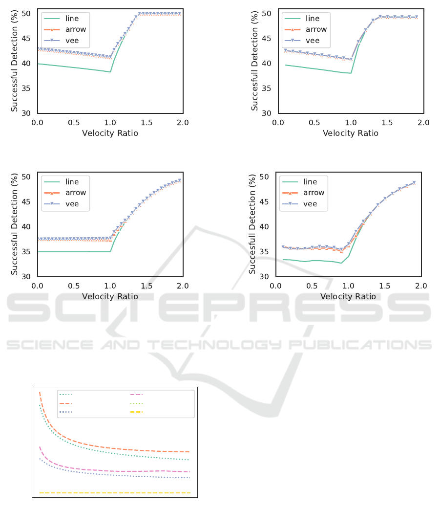
Figure 8: Comparisons of mathematical framework vs simulation results for entry-time aware and agnostic missions.
mathematical framework to calculate the aforemen-
tioned probabilities in various scenarios.
2 4 6 8 10 12 14 16 18 20
Corridor Length (km)
0
2
4
6
Improvement (%)
arrow, v
d
= 1
vee, v
d
= 1
arrow, v
d
= 1.1
vee, v
d
= 1.1
arrow, v
d
= 1.25
vee, v
d
= 1.25
Figure 9: Results of the experiment showing how the per-
formance depends on the length of the corridor. The vertical
axis shows the relative improvement of detection chance wrt
to the line formation.
To support the reproducibility of our research, we
publish the source code of the mathematical frame-
work and of this study in [redacted in initial submis-
sion to maintain anonymity]. We start by analyzing
the results presented in Fig. 8. First of all, for both
scenarios, the vee formation results in the best per-
formance, being slightly better than the arrow for-
mation. The line formation performing significantly
worse. Furthermore, in both cases, the formations
achieve the same performance starting from a velocity
ratio of around 1.25, which confirms the intuition that
for fast-moving search parties, the formation choice
is less important. For the velocity ratio above 1.5,
they converge to the 50 % of successful detections.
This observation matches the intuition that, with high
speed, the 50% of the targets that appear in front of
the formation will all be detected before they can es-
cape from the fleet detection range. Furthermore, the
results of the entry-time aware mission present a per-
haps counter-intuitive finding: if the searching drones
cannot move as fast as the target, it might be better to
slow them down even further. This can be explained
by the fact that moving slower gives more chances for
the targets appearing behind the formation to catch
up with the formation and the formation will not be
able to catch up to many targets appearing in front of
ICAART 2025 - 17th International Conference on Agents and Artificial Intelligence
478

it. This behavior does not appear in the entry-time
agnostic mission, where a target entrance time is in-
cluded.
In Fig. 9 we show how the performance in the
entry-time agnostic mission changes depending on
the corridor length. We present it as a relative im-
provement wrt to the line formation to emphasize the
benefits of choosing the correct formation. We show
the plots for multiple values of v
d
to show how this
plot changes in relation to the findings previously pre-
sented in Fig. 8. The obtained results are very intu-
itive: the longer the corridor, the lower the benefit of
choosing the better formation.
0.0 0.2 0.4 0.6 0.8 1.0 1.2 1.4
v
d
0
100
200
300
400
500
600
700
800
900
Group position when target appears (m)
Arrow
Vee
Figure 10: Results of the experiment showing which for-
mation outperforms the other according to different velocity
ratios and positions of the group when the target appears.
Finally, to explicitly address the question pre-
sented as the motivation of this research, we present
Fig. 10. It presents the difference in performance be-
tween the vee and arrow formation and could serve as
an easy way to choose which one to prefer, depend-
ing on the scenario at hand. The line formation is
not presented, as it is never performing better than the
aforementioned two.
4.4 Robotic Proof of Concept
Our proof of concept involves deploying a fleet of
six UAVs (specifically, Holybro PX4 Vision) in each
of the formations introduced above. The UAVs are
equipped with Arducam 12 MP, IMX477 camera with
an 80
◦
horizontal field of view, flying at an altitude of
50 meters with an exploration depth (corridor length)
of 1 kilometer. This setup was successfully tested
over a maritime environment to detect a target in the
sea and in a deserted area to detect a car using a
YOLO algorithm (Redmon et al., 2016), demonstrat-
ing that our model is applicable in realistic scenarios.
5 CONCLUSIONS
The mathematical framework presented in this paper
offers a convenient and efficient means of analyzing
the formation flights of a fleet of drones. It allows
for the estimation of the probability of target detec-
tion during a search mission. Specifically, it serves
as a valuable tool for selecting the most effective
formation in a given context. The proposed scenar-
ios demonstrate the practical value of this framework
in real-world applications such as search and rescue,
border surveillance, and environmental monitoring.
Although our initial experiments yielded promising
results, we are planning further in-field experiments
to gain insights and quantitatively validate the math-
ematical framework under realistic conditions and
across various scenarios.
REFERENCES
Afonso, F., Sohst, M., Diogo, C. M. A., Rodrigues, S. S.,
Ferreira, A., Ribeiro, I., Marques, R., Rego, F.
F. C., Sohouli, A., Portugal-Pereira, J., Policarpo, H.,
Soares, B., Ferreira, B., Fernandes, E. C., Lau, F., and
Suleman, A. (2023). Strategies towards a more sus-
tainable aviation: A systematic review. Progress in
Aerospace Sciences, 137:100878.
Anderson, B. D., Fidan, B., Yu, C., and Van der Walle, D.
(2008). UAV Formation Control: Theory and Appli-
cation. In Recent advances in learning and control,
volume 371 of Lecture Notes in Control and Informa-
tion Sciences, pages 15–33. Springer edition.
Antczak, A., Lasek, M., and Sibilski, K. (2022). Efficient
Positioning of Two Long-Range Passenger Aircraft
in Formation Flight. Transactions on Aerospace Re-
search, Nr 3 (268).
Atınc¸, G. M., Stipanovi
´
c, D. M., and Voulgaris, P. G.
(2020). A swarm-based approach to dynamic cov-
erage control of multi-agent systems. Automatica,
112:108637.
Bajec, I. L. and Heppner, F. H. (2009). Organized flight in
birds. Animal Behaviour, 78(4):777–789.
Chao, Z., Zhou, S.-L., Ming, L., and Zhang, W.-G. (2012).
UAV Formation Flight Based on Nonlinear Model
Predictive Control. Mathematical Problems in Engi-
neering, 2012:e261367. Publisher: Hindawi.
Cheng, T. M. and Savkin, A. V. (2009). Decentralized co-
ordinated control of a vehicle network for deployment
in sweep coverage. In 2009 IEEE International Con-
ference on Control and Automation, pages 275–279.
ISSN: 1948-3457.
de Souza, C., Newbury, R., Cosgun, A., Castillo, P., Vi-
dolov, B., and Kuli
´
c, D. (2021). Decentralized Multi-
Agent Pursuit Using Deep Reinforcement Learning.
IEEE Robotics and Automation Letters, 6(3):4552–
4559. Conference Name: IEEE Robotics and Au-
tomation Letters.
Formation Analysis for a Fleet of Drones: A Mathematical Framework
479

Dorigo, M., Floreano, D., Gambardella, L. M., Mondada,
F., Nolfi, S., Baaboura, T., Birattari, M., Bonani, M.,
Brambilla, M., Brutschy, A., Burnier, D., Campo,
A., Christensen, A. L., Decugniere, A., Di Caro,
G., Ducatelle, F., Ferrante, E., Forster, A., Gonzales,
J. M., Guzzi, J., Longchamp, V., Magnenat, S., Math-
ews, N., Montes de Oca, M., O’Grady, R., Pinciroli,
C., Pini, G., Retornaz, P., Roberts, J., Sperati, V., Stir-
ling, T., Stranieri, A., Stutzle, T., Trianni, V., Tuci,
E., Turgut, A. E., and Vaussard, F. (2013). Swar-
manoid: A Novel Concept for the Study of Hetero-
geneous Robotic Swarms. IEEE Robotics & Automa-
tion Magazine, 20(4):60–71. Conference Name: IEEE
Robotics & Automation Magazine.
Hartjes, S., Visser, H. G., and van Hellenberg Hubar,
M. E. G. (2019). Trajectory Optimization of Ex-
tended Formation Flights for Commercial Aviation.
Aerospace, 6(9):100. Number: 9 Publisher: Multi-
disciplinary Digital Publishing Institute.
Hespanha, J., Kim, H. J., and Sastry, S. (1999). Multiple-
agent probabilistic pursuit-evasion games. In Pro-
ceedings of the 38th IEEE Conference on Decision
and Control (Cat. No.99CH36304), volume 3, pages
2432–2437 vol.3. ISSN: 0191-2216.
Ivi
´
c, S., Crnkovi
´
c, B., Arbabi, H., Loire, S., Clary, P., and
Mezi
´
c, I. (2020). Search strategy in a complex and
dynamic environment: the MH370 case. Scientific Re-
ports, 10:19640.
Justh, E. W. and Krishnaprasad, P. S. (2002). A Simple
Control Law for UAV Formation Flying.
Kovacina, M., Palmer, D., Yang, G., and Vaidyanathan, R.
(2002). Multi-agent control algorithms for chemical
cloud detection and mapping using unmanned air ve-
hicles. In IEEE/RSJ International Conference on In-
telligent Robots and Systems, volume 3, pages 2782–
2788 vol.3.
Liu, H. Y., Chen, J., Huang, K. H., Cheng, G. Q., and Wang,
R. (2023). UAV swarm collaborative coverage con-
trol using GV division and planning algorithm. The
Aeronautical Journal, 127(1309):446–465. Publisher:
Cambridge University Press.
Mazdin, P., Barci
´
s, M., Hellwagner, H., and Rinner, B.
(2020). Distributed Task Assignment in Multi-Robot
Systems based on Information Utility. In 2020 IEEE
16th International Conference on Automation Science
and Engineering (CASE), pages 734–740. ISSN:
2161-8089.
Papatheodorou, S. and Tzes, A. (2018). Theoretical and
Experimental Collaborative Area Coverage Schemes
Using Mobile Agents.
Paul, T., Krogstad, T. R., and Gravdahl, J. T. (2008). Mod-
elling of UAV formation flight using 3D potential
field. Simulation Modelling Practice and Theory,
16(9):1453–1462.
Redmon, J., Divvala, S., Girshick, R., and Farhadi, A.
(2016). You Only Look Once: Unified, Real-Time
Object Detection. arXiv:1506.02640 [cs].
Saska, M., Von
´
asek, V., and P
ˇ
reu
ˇ
cil, L. (2013). Trajectory
Planning and Control for Airport Snow Sweeping by
Autonomous Formations of Ploughs. Journal of Intel-
ligent & Robotic Systems, 72(2):239–261.
Wang, X., Yadav, V., and Balakrishnan, S. N. (2007).
Cooperative UAV Formation Flying With Obsta-
cle/Collision Avoidance. IEEE Transactions on Con-
trol Systems Technology, 15(4):672–679. Conference
Name: IEEE Transactions on Control Systems Tech-
nology.
Wei, X. and Yanq, J. (2018). Optimal Strategies for Mul-
tiple Unmanned Aerial Vehicles in a Pursuit/Evasion
Differential Game. Journal Guidance, Control and
Dynamics, 41.
Yu, Y., Li, Z., Wang, X., and Shen, L. (2019). Bearing-
only circumnavigation control of the multi-agent sys-
tem around a moving target. IET Control Theory &
Applications, 13(17):2747–2757.
Zhai, C. and Hong, Y. (2012). Decentralized sweep cover-
age algorithm for uncertain region of multi-agent sys-
tems. In 2012 American Control Conference (ACC),
pages 4522–4527. ISSN: 2378-5861.
Zhai, C. and Hong, Y. (2013). Decentralized sweep cover-
age algorithm for multi-agent systems with workload
uncertainties. Automatica, 49(7):2154–2159.
ICAART 2025 - 17th International Conference on Agents and Artificial Intelligence
480
