Hierarchically Gated Experts for Efﬁcient Online Continual Learning

Kevin Luong

and Michael Thielscher

The University of New South Wales, Sydney, Australia

{kevin.luong, mit}@unsw.edu.au

Keywords:

Neural Networks, Machine Learning, Continual Learning, Mixture-of-Experts.

Abstract:

Continual Learning models aim to learn a set of tasks under the constraint that the tasks arrive sequentially

with no way to access data from previous tasks. The Online Continual Learning framework poses a further

challenge where the tasks are unknown and instead the data arrives as a single stream. Building on existing

work, we propose a method for identifying these underlying tasks: the Gated Experts (GE) algorithm, where a

dynamically growing set of experts allows for new knowledge to be acquired without catastrophic forgetting.

Furthermore, we extend GE to Hierarchically Gated Experts (HGE), a method which is able to efﬁciently

select the best expert for each data sample by organising the experts into a hierarchical structure. On standard

Continual Learning benchmarks, GE and HGE are able to achieve results comparable with current methods,

with HGE doing so more efﬁciently.

1 INTRODUCTION

Continual Learning, also known as Lifelong Learn-

ing, addresses the challenge of creating AI able to

continually learn and apply knowledge over long time

spans (Parisi et al., 2018). The biggest barrier to

achieving such an AI is catastrophic forgetting, where

previously learnt knowledge is lost due to interference

when acquiring new knowledge. In practice, this is

observed as a reduction in performance on existing

tasks when learning a new task.

In Continual Learning an agent is restricted from

seeing past data samples yet must correctly model

both past and present data. Whilst past data samples

are always forbidden, in many continual learning set-

tings the data is assumed to come from a series of sep-

arate distributions (tasks) with each sample labelled

according to its distribution (Kirkpatrick et al., 2017;

Lopez-Paz and Ranzato, 2017). This task identity

data is not available in the Online Continual Learning

setting, which is currently gaining attention as a more

useful extension to Continual Learning (Kirichenko

et al., 2021; Hihn and Braun, 2023).

Many Continual Learning techniques in both on-

line and ofﬂine settings aim to mitigate interference

between tasks, and thus catastrophic forgetting, by

employing a set of experts such that each expert is as-

sociated with a single task (Aljundi et al., 2017; Zhu

https://orcid.org/0009-0007-3362-9082

https://orcid.org/0000-0003-0885-2702

et al., 2022). The challenge, in online settings, is then

in selecting the correct expert during both training and

testing. We build on existing work in this area to pro-

pose our own method, which we name Gated Experts

(GE). More speciﬁcally, our algorithm can be seen as

an extension of Expert Gate (Aljundi et al., 2017) to

the online setting by detecting task switches as statis-

tically signiﬁcant deviations in the training loss. We

credit Zhu et al. (2022) for the idea to use the train-

ing loss as a task switch signal. However, we track

the loss and detect task switches in a different man-

ner to address shortcomings in the existing approach,

discussed in section 3.3.

The GE algorithm belongs to the class of

expansion-based methods, where the number of pa-

rameters dynamically grows as needed to learn new

tasks. In this area, the efﬁciency of an algorithm is

often optimised by reducing the number of parame-

ters, by pruning (Zhu et al., 2022) or other methods

(Yoon et al., 2018; Xu and Zhu, 2018). We instead

propose to organise the experts in a hierarchical man-

ner, so that only a subset of experts are required for

any given data sample. Thus, the inference time can

be improved. We name this extension Hierarchically

Gated Experts (HGE).

We evaluate GE on standard Continual Learning

benchmarks and show that it is competitive with the

state-of-the-art in Online Continual Learning. Then,

we create new Continual Learning scenarios involv-

ing a mixture of datasets to which we apply both GE

Luong, K. and Thielscher, M.

Hierarchically Gated Experts for Efﬁcient Online Continual Learning.

DOI: 10.5220/0013190000003890

Paper published under CC license (CC BY-NC-ND 4.0)

In Proceedings of the 17th International Conference on Agents and Artiﬁcial Intelligence (ICAART 2025) - Volume 2, pages 507-518

ISBN: 978-989-758-737-5; ISSN: 2184-433X

507

and HGE. We show that HGE is able to organise ex-

perts hierarchically, thus increasing efﬁciency, with

little loss in accuracy.

In summary, our contributions are:

• We present a novel method for task switch de-

tection to address shortcomings in an existing ap-

proach.

• We apply this method on existing work to pro-

pose the GE algorithm and empirically show it to

be competitive with the state-of-the-art in Online

Continual Learning.

• We propose hierarchical organisation, unexplored

in the literature thus far, as a means of improv-

ing the efﬁciency of expansion-based Continual

Learning methods. Our HGE extension improves

upon the efﬁciency of GE. We demonstrate the ex-

tension on bigger Continual Learning scenarios as

a proof-of-concept.

The rest of the paper is structured as follows. We

provide an overview of Continual Learning and cur-

rent methods in Section 2. Then, we present our ap-

proach to task switch detection and the GE algorithm

in section 3, and describe the HGE extension in sec-

tion 4. Our experimental setup and results are given

in Section 5, and we conclude with a summary and

discussion of future work in Section 6.

2 BACKGROUND

2.1 Continual Learning

There has been a wide array of approaches proposed

for continual learning. We provide a broad overview

of the continual learning landscape, but refer to sur-

veys for a taxonomy as well as a more comprehen-

sive coverage of these approaches (Parisi et al., 2018;

Wang et al., 2024). There exists three major cate-

gories of continual learning methods: architectural,

regularisation, and replay-based.

Architectural Approaches: aim to assign speciﬁc

model parameters to speciﬁc tasks, thus mitigating

catastrophic forgetting as each parameter is only ﬁt-

ted to one task. Often, there is a separate model, re-

ferred to as an expert, that is assigned to each task

to be learnt (Zhu et al., 2022; Lee et al., 2020). The

Expert gate (Aljundi et al., 2017) algorithm creates

a new expert for each task during training, as well

as an autoencoder to learn a representation for the

task. During test time, each sample is forwarded to

the expert corresponding to the autoencoder that best

recreates the sample. Alternatively, there exist ap-

proaches where the network is ﬁxed but binary masks

are learned to restrict each task to a subset of param-

eters (Kang et al., 2022; Wortsman et al., 2020). In

some cases, the task-speciﬁc parameters may not be

stored and instead generated by a meta-model known

as a hypernetwork (HN) (Hemati et al., 2023).

Regularisation Techniques: constrain updates to

previous parameters to preserve learnt knowledge. In

many popular approaches, including Elastic Weight

Consolidation (Kirkpatrick et al., 2017), Gradient

Episodic Memory (Lopez-Paz and Ranzato, 2017)

and Synaptic Intelligence (Zenke et al., 2017), this is

achieved by applying a loss to penalise changes to pa-

rameters considered to be important. Learning with-

out Forgetting (Li and Hoiem, 2017) is another pop-

ular regularisation technique which records a model’s

output on new data and uses this as a pseudo-label to

preserve the model’s capabilities.

Replay-Based Approaches: involve saving and re-

training on previously seen data. Generally, it is as-

sumed that only a small subset of training samples

can be stored, in which case the main challenge is in

selecting the best samples to store (Chaudhry et al.,

2019; Lopez-Paz and Ranzato, 2017). Other works

in this area do not explicitly store the samples, but

instead train a network to recreate them (Shin et al.,

2017). Replay is commonly incorporated into contin-

ual learning algorithms, even if the works themselves

are focused on other aspects (Zhu et al., 2022; Hihn

and Braun, 2023; Kirichenko et al., 2021).

Continual learning scenarios are often categorised

as either domain incremental or class incremental

(Wang et al., 2024), although other categories exist.

In the domain incremental setting, the inputs for each

task come from a different distribution and the output

space is shared. In the class incremental setting, the

inputs come from the same distribution and the output

space is disjoint.

2.2 Online Continual Learning Methods

In Online Continual Learning, also known as Task-

Free or Task-Agnostic Continual Learning, task iden-

tities are not provided during training nor testing.

provide an overview of some of the main approaches

proposed in this area, which we will also use to com-

pare with our method.

Bayesian Gradient Descent (BGD) is an early

work in the Online Continual Learning setting (Zeno

et al., 2018). The authors build on previous work

in online variational Bayesian learning to propose a

Online Continual Learning may also refer to scenar-

ios where each training sample is only shown once, i.e. one

epoch per task (Wang et al., 2024). We do not consider this

case and only focus on learning without task identities.

ICAART 2025 - 17th International Conference on Agents and Artiﬁcial Intelligence

508

closed-form update rule for the mean and variance of

each parameter. Catastrophic forgetting is naturally

mitigated as the posterior distribution of parameters,

which captures all currently learnt knowledge, is used

as the prior in the next training step.

Lee et al. (2020) formulate the Continual Learn-

ing problem as a stream of data from a mixture dis-

tribution and propose the Continual Neural Dirichlet

Process Mixture (CN-DPM) algorithm where a set of

experts, each containing a discriminative and a gen-

erative component, models the overall mixture distri-

bution. In CN-DPM, new experts are added in a prin-

cipled manner using Sequential Variational Approxi-

mation (Lin, 2013).

The Hybrid generative-discriminative approach

to Continual Learning for classiﬁcation (HCL)

(Kirichenko et al., 2021) jointly models the distribu-

tion of the input data and labels for each task using a

normalising ﬂow. Three model statistics are tracked

for each existing task and a task switch is detected if

all three statistics lie outside the normal range. To

prevent catastrophic forgetting, the authors propose

using generative replay as well as a novel functional

regularisation loss to enforce similar mappings to a

snapshot taken on task switch.

In Task-Agnostic continual learning using Multi-

ple Experts (TAME) (Zhu et al., 2022), a set of ex-

perts is maintained where each is associated with a

training task. Task switches are detected using a sta-

tistically signiﬁcant deviation in the training loss, at

which point a new expert is created. Each expert also

maintains a small buffer of training samples, which

are used to prune experts as well as train a selector

network to choose the correct expert during test time.

Hierarchical Variational Continual Learning

(HVCL) (Hihn and Braun, 2023) extends VCL

(Nguyen et al., 2018) to the task-agnostic setting

using the Sparsely Gated Mixture-of-Experts layer

(Shazeer et al., 2017). Dynamic path selection

through the HVCL model effectively produces

distinct experts to solve different tasks. The authors

introduce novel diversity objectives to better allo-

cate experts to tasks, thus mitigating catastrophic

forgetting.

Sparse neural Networks for Continual Learning

(SNCL) (Yan et al., 2022) is a method that com-

bines sparse networks, where unused parameters are

reserved for future tasks, with a novel experience re-

play approach where the intermediate network activa-

tions are stored in addition to the sample. The sparsity

is enforced by a variational Bayesian prior applied to

the activation of each neuron. The proposed experi-

ence replay approach, named Full Experience Replay,

allows for the priors to be more effectively optimised.

Finally, in Dynamically Expandable Representa-

tion (DER) (Yan et al., 2021), a super-feature extrac-

tor is repeatedly expanded to accommodate new data.

Catastrophic forgetting is mitigated as the older pa-

rameters are frozen, whilst pruning reduces redun-

dancy in the added parameters. As the super-feature

extractor is expanded, the classiﬁer is continually

ﬁnetuned using experience replay.

3 ONLINE CONTINUAL

LEARNING

In the Online Continual Learning paradigm, training

data D

train

= {(x

)}

i=1

in the form of input-output

pairs arrives sequentially such that when (x

) is

seen, {(x

)}

i−1

j=1

cannot be accessed. The goal is

to learn a model f of inputs to outputs with no infor-

mation given about the data generating process. Fol-

lowing training, the model is judged on testing data

test

= {(x

)}

i=1

by comparing the expected (y

)

and model ( f (x

)) outputs.

We follow the common assumption (Hihn and

Braun, 2023; Kirichenko et al., 2021) that there exists

a set of distributions (tasks) from which the data is

generated and that they arrive in a sequence (possibly

with repetitions) with a hard boundary between each

task. Formally, there exists a constant C such that if

) belongs to task m and (x

i+1

) belongs to

task m+1, then {(x

)}

i+C

j=i+1

belongs to task m+1.

At a hard task boundary a large and sustained in-

crease in the training loss can be expected. Task-

Agnostic continual learning using Multiple Experts

(TAME) (Zhu et al., 2022) (cf. Section 2.2) is a

method for detecting these boundaries by tracking the

loss of a single active expert on incoming samples.

A threshold for acceptable losses is calculated using

the mean and standard deviation of the loss over a

moving window. When the incoming loss, which is

smoothed using an exponentially weighted moving av-

erage (EWMA), exceeds this threshold, a task switch

is detected. The active expert is then switched to the

correct expert or to a new expert if the incoming task

is unseen.

In this section, we propose a method for On-

line Continual Learning that, like TAME, leverages

statistically signiﬁcant increases in the training loss

to detect task switches. First we describe our ap-

proach to task switch detection (Section 3.1). Then

we show how this can be applied to extend the Expert

Gate algorithm (Aljundi et al., 2017) to produce our

Gated Experts (GE) algorithm (Section 3.2). We also

provide a comparison between TAME and GE (Sec-

tion 3.3).

Hierarchically Gated Experts for Efﬁcient Online Continual Learning

509

3.1 Detecting Task Switches in Online

Continual Learning

Given an expert and an input sample, we must deter-

mine if the sample belongs to the same task on which

the expert was trained. To do so, for each expert we

maintain an EWMA of the value and deviation of the

training loss. Given n training losses L, the mean µ

and standard deviation σ are deﬁned as follows:

← L

← α µ

n−1

+ (1 −α)L

,n > 1

← 0

← L

−L

← α σ

n−1

+ (1 −α)(L

−µ

n−1

),n > 2

α is the smoothing factor for the EWMA and should

be set relatively high (we use α = 0.9) to reduce the

impact of noise in the training loss. The mean and

standard deviation of the training loss are combined

with a threshold hyperparameter ε to produce an up-

per bound on the training loss:

µ + εσ

If the loss of the given input sample is above this up-

per bound, we assume one of three possibilities:

1. The sample belongs to the same task as the expert

but is an outlier.

2. The sample belongs to another task.

3. The sample belongs to the same task as the ex-

pert but instability in the training process has tem-

porarily increased the loss.

To determine which of these is correct, we set aside

the input sample in a buffer (the high-loss buffer) and

await further samples. If the training loss immediately

returns below the threshold, the ﬁrst scenario has oc-

curred as the other two can be ruled out.

It is clear that the second scenario will result in a

consistently high training loss, and we also expect to

see this trend in the third scenario; if training insta-

bility has left the expert in a state where it produces

high training losses, setting aside the input samples

prevents the expert from exiting such a state. Thus, if

a consistently high training loss is observed, we must

determine if the second or third scenario has occurred.

The second and third scenarios can be differenti-

ated with the aid of a small buffer of samples on which

the expert was trained. Samples from this buffer are

compared to the high-loss samples in a statistical test

to determine if they belong to the same distribution.

First, the training loss is calculated for all samples.

We hypothesise that the loss is normally distributed

because in practice, each loss is the mean over a batch

of training examples and as a result the Central Limit

Theorem can be applied. Thus, we apply a simple Z-

test: Let µ

and σ be the mean and standard deviation

of the n losses from the samples in the expert buffer,

and µ

be the mean of the losses from the high-loss

buffer, then the standard error SE and Z-score ZS are

calculated as:

SE = σ/

√

ZS = |µ

−µ

|/SE

If ZS is above a threshold hyperparameter ε

review

, then

we assume scenario 2 has occurred, and scenario 3

otherwise.

3.2 Gated Experts

Detecting switches in the input task allows for the Ex-

pert Gate algorithm (Aljundi et al., 2017) to be ex-

tended to the Online Continual Learning setting. We

name this extension Gated Experts (GE) and provide

the pseudocode in Algorithm 1. In GE, a set of ex-

perts (initially one) is maintained with each expert

corresponding to a single task out of all tasks seen

so far. Associated with each expert is an autoencoder

that is trained on the same data. As each training sam-

ple arrives, it is forwarded to the most relevant expert

deﬁned by the lowest autoencoding loss. Thus, task

switches between existing tasks are handled. When

a task switch is detected, we can assume that the in-

coming task is new and thus create a new expert.

When a new expert is created, it is likely that fu-

ture samples from the same task will not be correctly

forwarded to said expert until the associated autoen-

coder is adequately trained. GE addresses this prob-

lem by maintaining a separate set of newly created

experts. When a sample is forwarded to an expert and

found to not belong to said expert, we check if it be-

longs to a newly created expert before setting it aside.

Thus, the following events will occur when samples

from a new task arrive:

1. The samples are forwarded to one or more exist-

ing experts, found to have a high loss and thus set

aside in the high-loss buffer.

2. A task switch is detected due to a consistently

high loss, and a new expert is created and trained

on the samples in the high-loss buffer.

3. Further samples from the new task arrive and are

forwarded to the same experts as in Step 1.

4. The samples are redirected to the new expert

rather than sent to the high-loss buffer.

During the ﬁnal step, we also track whether the

loss of the sample on the new expert was greater or

lower than on the existing expert. When the loss on

ICAART 2025 - 17th International Conference on Agents and Artiﬁcial Intelligence

510

Data: (x

) = the incoming training sample

E = the set of existing experts

new

= the set of newly created experts

R = a buffer to store recent samples

append (x

) to R

best

← GE forward(E, (x

)) // returns the

expert with lowest autoencoding loss

if Loss(e

best

, (x

)) > e

best

.threshold then

if there exists e

new

in E

new

such that

Loss(e

new

, (x

)) ≤ e

new

.threshold then

train e

new

on (x

)

promote e

new

if the conditions are met

else

mark (x

) as a high-loss sample

end

else

train e

best

on (x

)

end

// Process outliers

if R is not full then

return

end

last

) ← the oldest sample in R

if (x

last

) is marked as high-loss then

last

← the expert that was trained on the

previous sample to (x

last

)

train e

last

on (x

last

)

end

remove (x

last

) from R

last

) ← the new oldest sample in R

// Detect task switches

if every remaining entry in R is a high-loss sample

then

last

← the expert with the lowest

autoencoding loss on (x

last

)

test the loss of e

last

on the samples in R and

the samples in e

last

.replay buffer

if the losses are statistically different then

create a new expert e

new

train e

new

on the samples in R

else

train e

last

on the samples in R

end

remove all samples from r

end

Algorithm 1: Pseudocode for the GE algorithm.

the new expert is consistently lower, then the new

expert can be promoted: the expert is removed

from the set of newly created experts and treated

as a regular expert. The promotion condition is

met when the proportion of lower losses in the last

promotion window samples exceeds ε

promotion

. In

GE, we set promotion window = 50 and ε

promotion

0.5.

A relatively low value of ε

promotion

is possible

as GE does not require perfect accuracy when for-

warding samples. Under the assumption of hard task

boundaries, adjacent samples are highly likely to be-

Data: (x

) = the incoming sample

E = the tree of existing experts

Result: e

best

= the expert with the lowest

autoencoding loss on (x

)

n ← the root node of E

while True do

if n has no children then

return

end

c ← the node in n.children with the lowest

AE Loss(c.expert, (x

))

if e

best

does not yet exist or AE Loss(c.expert,

)) < AE Loss(e

best

, (x

)) then

best

← c.expert

else

return

end

Algorithm 2: HGE forward - In HGE, the most relevant

expert for a given sample is found by starting at the root

and repeatedly choosing the best child.

long to the same task. When a sample is forwarded to

the wrong expert, a temporary high-loss is observed

similar to an outlier. In both cases, the sample will be

assigned to the same expert as the previous sample.

3.3 Comparison to TAME

The main advantage of GE over TAME is in the

high-loss buffer. Performing a statistical test be-

fore detecting a task switch greatly reduces the false-

positive rate, as we show experimentally in Sec-

tion 5.1. In addition, in TAME one or more samples

may be wrongly trained on the active expert before the

EWMA of the loss exceeds the acceptable threshold.

This is prevented in GE as samples over the threshold

are immediately set aside.

Another difference is in the lack of an active ex-

pert in GE. By assigning each sample to the expert

with the lowest autoencoding loss, the algorithm is

simpliﬁed as task switches between existing tasks are

a non-factor. In practice, the last-used expert could

be tracked to improve the efﬁciency of GE. If an in-

coming sample has a loss within the threshold of the

last-used expert, then we can assign it to said expert

without calculating all of the autoencoding losses.

4 HIERARCHICALLY GATED

EXPERTS

In GE the autoencoding losses are used as a measure

of the suitability of an expert to a given sample. We

hypothesise the existence of relationships between ex-

perts such that the suitability of an expert can be esti-

Hierarchically Gated Experts for Efﬁcient Online Continual Learning

511

mated from the autoencoding losses of its peers. For

example, if experts A and B are both trained on tasks

in the same domain then we can expect that they will

produce a low autoencoding loss for any sample from

said domain. Thus, if expert A produces a high au-

toencoding loss then we can assume that the sample

originates from a different domain, and that expert B

will likewise be unsuitable.

We propose the idea of organising experts hierar-

chically to exploit these relationships and improve the

speed with which an expert can be selected for a given

sample. Our algorithm, named Hierarchically Gated

Experts (HGE), is an extension to GE where the set

of existing experts is instead a tree with each node

(except the root) corresponding to a speciﬁc expert.

Given a sample, we traverse the tree by following the

child with the lowest autoencoding loss at each step.

We stop when a leaf node is reached or when the cur-

rent node has a lower autoencoding loss than each of

its children. The ﬁnal node is then considered to cor-

respond to the expert with the overall lowest autoen-

coding loss. Thus, an expert can be selected with-

out calculating the autoencoding loss for all experts.

The pseudocode for the traversal is provided in Algo-

rithm 2.

The tree of experts is built iteratively. As each

expert is promoted, it is added to the tree such that

samples from the corresponding task will be correctly

assigned to the expert. This can be trivially accom-

plished by adding the expert as a child of the root, so

that its autoencoding loss will always be calculated.

However, such a strategy will produce a completely

ﬂat tree and be equivalent to the GE algorithm. Thus,

we instead aim to insert the expert as deeply as pos-

sible while maintaining assignment accuracy. As a

newly created expert is trained, we track the traversal

paths taken by every sample the expert is given. When

the expert is promoted, it is inserted as a child of the

lowest common ancestor (LCA) of all traversal paths.

Outlier paths, which are only taken a few times, are

excluded according to the promotion path threshold

hyperparameter. The pseudocode for expert promo-

tion is provided in Algorithm 3.

When a new expert is added to the tree, it is pos-

sible that it will mask some of the existing experts,

causing catastrophic forgetting. With reference to

Figure 1, expert 0 will mask expert 3 if, on samples

from task 3, expert 0 has a lower autoencoding loss

than expert 1. When an expert is inserted, all descen-

dants of siblings can potentially be masked. To miti-

gate this, the replay buffer of each potentially masked

expert is used to estimate if masking will occur. If any

replay samples are incorrectly assigned to the new ex-

pert, then a new node corresponding to the masked ex-

root

0 1

2 3 4

Figure 1: An example tree generated by HGE. Each node

corresponds to a different expert.

Data: E = the tree of existing experts

new

= the expert to be promoted

paths = a list of the unique paths taken by the

samples on which e

new

was trained. Each path also

contains a count of the number of times it was

taken.

new

node ← a new node with e

new

node.expert =

new

and no children

if there is only one expert in E then

add e

new

node as a child of the root node of E

return

end

// Insert expert into tree

sort paths by count in decreasing order

for p in paths do

sum ← the cumulative sum of counts up to

and including p

total ← the sum of all counts in paths

if sum > promotion path threshold * total

then

remove all remaining members of paths

end

parent ← the LCA of all remaining p in paths

add e

new

node as a child of parent

// Add backward connections

possible overwrites ← {}

for each descendant n of parent excluding

new

node do

add n.expert to possible overwrites

end

for e

overwr ite

in possible overwrites do

if there exists (x

) in e

overwr ite

.replay buffer

where HGE forward(E, (x

)) = e

new

then

add a node n as a child of e

new

node with

n.expert = e

overwr ite

end

Algorithm 3: Expert Promotion in HGE.

pert is added as a child of the new expert. We choose

to create a new node rather than add a connection to

the existing node so that we do not unnecessarily add

the descendants of the masked expert.

The hierarchical organisation of experts compli-

cates the promotion process. In GE, there is a wide

ICAART 2025 - 17th International Conference on Agents and Artiﬁcial Intelligence

512

range of possible promotion times as the algorithm is

able to handle samples being forwarded to the wrong

expert. In HGE, however, it is much easier for the pro-

motion of an expert to be performed too early. When

an expert is promoted in HGE, it is added to the tree

in a way that exploits the relationship between the au-

toencoders. As the expert continues to train, these

relationships may change and the expert may begin

to mask others, causing catastrophic forgetting. Thus,

a higher ε

promotion

is preferred. On the other hand,

a promotion threshold that is too high may never be

met.

In our experiments, we set a separate ε

promotion

for

each scenario roughly equal to the accuracy achieved

at the end of training. This approach works reason-

ably well, but it does break the Online Continual

Learning paradigm as we are using task-speciﬁc in-

formation. The promotion time is part of a larger

problem of dealing with changing relationships be-

tween experts, which we leave as a problem for future

research.

5 EXPERIMENTS

In this section, we experimentally evaluate our ap-

proach to task switch detection in the Online Con-

tinual Learning setting. We also perform controlled

experiments with GE and HGE to determine the im-

pact of hierarchical expert organisation on the gating

accuracy. Finally, we validate GE and HGE on Online

Continual Learning benchmarks.

We use widely known and commonly adopted

Continual Learning scenarios in our experiments:

Permuted MNIST (PMNIST). The MNIST dataset

(Lecun et al., 1998) is used as the ﬁrst task in this sce-

nario. Each subsequent task reuses MNIST, but with

the pixels in each image randomly permuted. The per-

mutations are kept consistent within each task. There

are 20 tasks in total.

Split MNIST (SMNIST). The MNIST dataset is split

into 5 tasks, each containing 2 classes.

Split CIFAR-10 (CIF10). The CIFAR-10 dataset

(Krizhevsky, 2012) is split into 5 tasks, each contain-

ing 2 classes.

Split CIFAR-100 (CIF100). The CIFAR-100 dataset

is split into either 10 or 20 tasks, each with the same

number of classes.

Split Tiny Imagenet (ImgNet). The Tiny Imagenet

dataset is a subset of Imagenet (Russakovsky et al.,

2015) containing images from 200 classes. We ran-

domly select 100 classes which are then evenly split

into either 10 or 20 tasks.

We also use scenarios that are both class-incre-

mental and domain-incremental. Each scenario in-

volves two datasets where the classes are split evenly

into tasks. The tasks are presented in an alternating

fashion; the ﬁrst task from the ﬁrst dataset, then the

ﬁrst task from the second dataset, then the second task

from the ﬁrst dataset, and so on. The scenarios are:

MNIST and Kuzushiji-MNIST (MNIST-

KMNIST). We split the MNIST dataset and

Kuzushiji-MNIST (KMNIST) dataset (Clanuwat

et al., 2018) into 5 tasks each, for a total of 10 tasks.

MNIST and CIFAR-10 (MNIST-CIF10). Similar

to the previous scenario, we split each dataset into 5

tasks each.

CIFAR-10 and Inverse CIFAR-10 (CIF10-INV).

We split each dataset into 5 tasks. To produce the In-

verse CIFAR-10 dataset, we invert the colour of every

pixel. The dataset is otherwise identical to CIFAR-10.

CIFAR-100 and Tiny Imagenet (CIF-ImgNet).

Each dataset is split into 10 tasks. Only 100 ran-

domly selected classes are used from the Tiny Ima-

genet dataset.

We use two variants of experts in our experiments.

In the PMNIST, SMNIST and MNIST-KMNIST sce-

narios, both the base model and the autoencoder are

multi-layer perceptrons (MLP). Otherwise, we use

Resnet-18 (He et al., 2015) as the base model and a

convolutional autoencoder. We provide the full details

of the dataset preprocessing, models used and hyper-

parameters in the Appendix.

5.1 Task Switch Detection

Table 1: The number of task switch detection errors per

task, categorised as false positives (FP) or false negatives

(FN). Cases with runaway expert creation are marked DNF

(Did Not Finish). CIFAR (all) and Imagenet (all) refer to all

scenarios tested purely on these datasets.

GE GE w/o review TAME

Scenario FP FN FP FN FP FN

PMNIST 0 0 0 0 0 0

SMNIST 0 0 0 0 0.04 0.04

CIFAR (all) 0 0 DNF DNF DNF DNF

Imagenet (all) 0 0 DNF DNF DNF DNF

MNIST-KMIST 0 0.04 0 0 0 0

MNIST-CIF10 0 0 DNF DNF DNF DNF

CIF10-INV 0 0 DNF DNF DNF DNF

CIF-ImgNet 0 0 DNF DNF DNF DNF

We ﬁrst test the effectiveness of our approach to task

switch detection. In each scenario, we observe the

creation of new experts and record cases where an

abnormal number of experts is created for a task.

Each additional expert is recorded as a false posi-

tive, whereas the case where no expert is created is

recorded as a false negative. When runaway expert

creation is observed (more than ﬁve per task), we ter-

Hierarchically Gated Experts for Efﬁcient Online Continual Learning

513

Table 2: The accuracy and efﬁciency of different approaches to organising the expert tree. Acc refers to the percentage of

batches which were assigned to the correct expert, whilst Exp is the average number of experts queried.

GE HGE Upper

Scenario Acc Exp Acc Exp Acc Exp

PMNIST 100.0 ±0.0 20 99.76 ±0.11 11.25 ±1.02 99.7 ±0.19 8.05 ±0.13

SMNIST 100.0 ±0.0 5 98.26 ±1.4 3.83 ±0.21 99.75 ±0.56 3.56 ±0.09

CIF10 95.25 ±5.11 5 95.0 ±5.66 4.17 ±0.55 95.0 ±5.66 3.85 ±0.38

CIF100(10) 77.25 ±2.05 10 76.75 ±1.9 9.49 ±0.85 75.0 ±4.59 8.02 ±0.33

CIF100(20) 83.25 ±8.08 20 82.75 ±7.52 17.55 ±1.43 84.0 ±8.59 12.84 ±0.74

ImgNet(10) 61.0±13.3 10 61.0 ±13.3 9.7 ±0.42 59.0 ±12.57 8.47 ±0.5

ImgNet(20) 73.5±5.76 20 73.5 ±5.76 19.02 ±0.93 73.5 ±2.85 15.03 ±0.6

MNIST-KMIST 95.25 ±5.94 10 95.25 ±5.94 6.42 ±0.57 95.01 ±5.72 5.13 ±0.09

MNIST-CIF10 98.88 ±0.52 10 98.75 ±0.77 5.29 ±0.1 98.4 ±1.01 4.92 ±0.16

CIF10-INV 98.25 ±0.93 10 97.88 ±0.71 6.62 ±0.99 98.0 ±0.93 5.31 ±0.19

CIF-ImgNet 68.88 ±1.49 20 68.88 ±1.49 19.06 ±0.81 68.38 ±1.44 15.6 ±0.65

minate the experiment early. We compare the GE al-

gorithm with TAME and also perform an ablation test

(GE w/o review) where we apply GE but do not per-

form a statistical test before creating a new expert.

Our results are summarised in Table 1. The low

error rate of GE across all scenarios demonstrates the

efﬁcacy of our approach to task switch detection. The

TAME and ablation test results reﬂect the nature of

the base models used in our experiments. The 3-

layer MLP is relatively stable during training, and as

a result we see very few errors in the pure MNIST

scenarios. On the other hand, our Resnet-18 model

has high instability, which causes runaway expert cre-

ation. These results show the importance of the statis-

tical test in differentiating between spikes in the loss

due to training instability and spikes due to data from

a new task.

We observed a small number of false negatives for

GE in the MNIST-KMNIST scenario. Upon analysis,

we found that the algorithm was able to re-use an ex-

isting expert with no loss in accuracy.

In our experiments, we observed much higher

z-scores than expected; over 20,000 during task

switches and up to 10 during some spikes in the train-

ing loss. Thus, our assumption that the training loss

is normally distributed does not hold well in prac-

tice. However, we still saw a clear separation between

the z-scores in both situations, and tuning the z-score

threshold hyperparameter ε

review

was not necessary.

We set ε

review

to a relatively high value and found this

worked for all scenarios.

5.2 Hierarchical Organisation

We aim to determine the impact of hierarchical or-

ganisation on the accuracy and efﬁciency of the ex-

pert selection process. We control for other factors

in Online Continual Learning, such as training sam-

ples being assigned to the wrong expert, by instead

training a separate expert on each task. We only mea-

sure the accuracy with which a sample is assigned to

the correct expert and do not consider the classiﬁca-

tion accuracy. We measure the cost of a tree as the

number of experts queried for a given sample. After

all experts are trained, we apply three approaches to

expert organisation:

GE. The experts are organised in a fully ﬂat tree.

HGE. In the same manner as the HGE algorithm, a

tree of experts is built by incrementally adding experts

according to task order. As each expert is trained sep-

arately, we do not have any traversal paths to track.

Instead, when an expert is added to the tree the traver-

sal paths are calculated for all training samples in the

corresponding task.

Upper. The HGE algorithm is run a large number of

times (1000) with a randomised task order, and the

accuracy and cost of each generated tree is recorded.

We then select the tree with the lowest cost and an

accuracy at least as high (approximately) as the GE

tree. This approach estimates the best possible tree

given the trained experts.

Our results are shown in Table 2. Both the HGE

and Upper approaches are able to produce trees with

close to optimal accuracies. In general, the cost re-

duction with HGE is dependent on the expert selec-

tion accuracy, with a markedly lower cost in scenar-

ios where the accuracy is high. This trend is also ob-

served with the Upper strategy, but to a lesser extent

as there is a decent cost reduction even when the se-

lection accuracy is low.

We also provide a statistical analysis of the accu-

racies and costs of the trees generated during the Up-

per strategy. We analyse the spread of the accuracy

and cost as well as the correlation between the two.

The results are provided in Table 3. We observe a low

but positive level of correlation across the board. We

believe that deeper trees are able to have a lower cost,

but may also suffer a lower accuracy as deeper nodes

have a higher chance of being masked.

We observe a very low level of spread in the accu-

ICAART 2025 - 17th International Conference on Agents and Artiﬁcial Intelligence

514

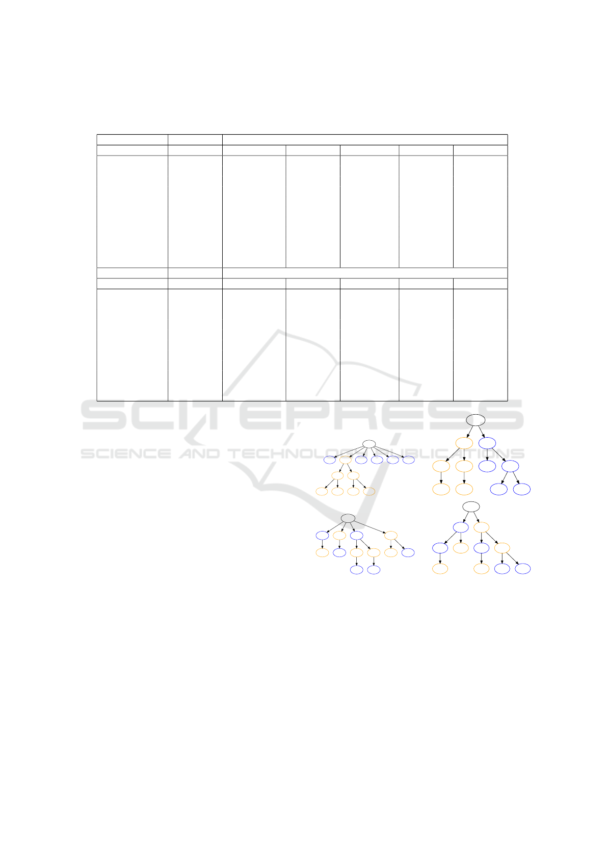
Table 3: A statistical analysis of the accuracy and query costs of all trees generated while ﬁnding an upper bound. PCC and

SCC are respectively the Pearson and Spearman correlation coefﬁcients, whilst MAD is the median absolute deviation. Each

metric is computed over all trees generated for a set of experts, then averaged across every set.

Acc

Scenario PCC Mean STD Median IQR MAD

PMNIST 0.13 ±0.06 99.57 ±0.04 0.45 ±0.08 99.71 ±0.03 0.39 ±0.07 0.19 ±0.0

SMNIST 0.3 ±0.19 99.55 ±0.48 0.7 ±0.6 100.0 ±0.0 0.72 ±1.06 0.0 ±0.0

CIF10 0.02 ±0.03 95.08 ±5.46 0.28 ±0.41 95.12 ±5.38 0.25 ±0.56 0.12 ±0.28

CIF100(10) 0.55 ±0.19 77.03 ±1.98 0.53 ±0.13 77.25 ±2.05 0.25 ±0.56 0.0 ±0.0

CIF100(20) 0.13 ±0.18 83.07 ±7.93 0.86 ±0.09 83.25 ±8.08 0.25 ±0.56 0.0 ±0.0

ImgNet 10) 0.11 ±0.29 60.97 ±13.28 0.39 ±0.2 61.0 ±13.3 0.0 ±0.0 0.0 ±0.0

ImgNet(20) 0.18 ±0.22 73.42 ±5.6 1.06 ±0.24 73.5 ±5.76 0.0 ±0.0 0.0 ±0.0

MNIST-KMIST 0.09 ±0.12 95.13 ±5.91 0.36 ±0.1 95.25 ±5.94 0.12 ±0.28 0.0 ±0.0

MNIST-CIF10 0.01 ±0.08 98.78 ±0.57 0.21 ±0.26 98.88 ±0.52 0.12 ±0.28 0.0 ±0.0

CIF10-INV 0.14 ±0.12 98.03 ±0.84 0.52 ±0.17 98.25 ±0.93 0.12 ±0.28 0.12 ±0.28

CIF-ImgNet 0.31 ±0.12 68.77 ±1.47 0.44 ±0.14 68.88 ±1.49 0.0 ±0.0 0.0 ±0.0

Exp

Scenario SCC Mean STD Median IQR MAD

PMNIST 0.17 ±0.08 11.32 ±0.32 1.45 ±0.14 11.16 ±0.34 1.97 ±0.22 0.97 ±0.1

SMNIST 0.36 ±0.21 4.08 ±0.09 0.32 ±0.03 4.07 ±0.15 0.41 ±0.02 0.26 ±0.07

CIF10 0.03 ±0.07 4.29 ±0.36 0.31 ±0.05 4.25 ±0.33 0.55 ±0.17 0.22 ±0.12

CIF100(10) 0.54 ±0.21 9.72 ±0.14 0.39 ±0.09 9.87 ±0.29 0.45 ±0.3 0.1 ±0.23

CIF100(20) 0.12±0.2 17.56 ±0.89 1.37 ±0.11 17.65 ±0.97 1.78 ±0.18 0.88 ±0.12

ImgNet 10) 0.05 ±0.31 9.86 ±0.1 0.26 ±0.12 10.0 ±0.0 0.13 ±0.29 0.0 ±0.0

ImgNet(20) 0.15 ±0.21 19.07 ±0.33 0.91 ±0.18 19.19 ±0.31 1.25 ±0.35 0.64 ±0.12

MNIST-KMIST 0.1 ±0.12 6.51 ±0.18 0.64 ±0.09 6.46 ±0.2 0.87 ±0.19 0.45 ±0.07

MNIST-CIF10 0.02 ±0.1 5.91 ±0.13 0.72 ±0.04 5.62 ±0.13 0.94 ±0.12 0.34 ±0.05

CIF10-INV 0.14 ±0.13 7.25 ±0.28 0.85 ±0.13 7.22 ±0.32 1.18 ±0.18 0.57 ±0.08

CIF-ImgNet 0.27 ±0.13 19.37 ±0.14 0.73 ±0.09 19.62 ±0.35 1.02 ±0.27 0.38 ±0.35

racies of the trees. The spread of the costs is higher

but still relatively low. Thus, we conclude that HGE is

not overly affected by the task order and is generally

able to organise the experts with close to the optimal

possible efﬁciency and cost.

A manual examination of the trees conﬁrms these

ﬁndings, as the HGE trees share many similarities

with the Upper trees. Figure 2 showcases this; both

HGE and Upper organise the experts according to do-

main in CIF10-INV, and in MNIST-KMNIST we see

identical connections such as between experts 7 and 3

or 2 and 5.

5.3 Continual Learning Benchmarks

We evaluate the overall efﬁcacy of GE and HGE by

providing a benchmark of the accuracies achieved by

these algorithms in an Online Continual Learning set-

ting. We also provide an estimate of the accuracy that

can be achieved given the base models used. The Sep-

arate method creates a separate model for each task

and uses task information to assign the samples, thus

serving as an upper bound.

Our results are presented in Table 4 and 5. We

measure accuracy as the average accuracy achieved

over all tasks at the end of training. We also report

the accuracy with which batches were assigned to the

correct expert (Gate Acc). During training, we track

root

0 1 2 4 6 8

3 9

5 7 5 7

root

7 8

1 5

9 3

0 4

2 6

root

0 1 2 7

9 4 3 5

6 8

3 6

root

0 7

4 9

2 3

5 6 8

Figure 2: Examples of trees generated by HGE and Upper.

Clockwise starting from the top-left: HGE on CIF10-INV,

Upper on CIF10-INV, Upper on MNIST-KMNIST, HGE on

MNIST-KMNIST. The nodes are coloured according to the

domain.

the samples assigned to each expert and record an as-

sociation between an expert and a task if the expert

was trained on at least 10% of the samples in the

task. During testing, we then measure the percent-

age of samples assigned to the correct expert. Finally,

we also report the average number of experts queried

during testing.

For comparison, we also provide the accuracy

Hierarchically Gated Experts for Efﬁcient Online Continual Learning

515

Table 4: Accuracy on continual learning benchmarks (%).

Method PMNIST SMNIST CIF10 CIF100(10) CIF100(20) ImgNet(10) ImgNet(20)

Separate 97.9 ±0.0 99.44 ±0.15 93.1 ±2.03 70.96 ±0.32 80.1 ±0.89 53.76 ±1.04 67.3 ±0.62

GE 97.9 ±0.07 99.54±0.09 89.06 ±4.05 51.96 ±6.31 65.62±5.76 31.02 ±5.3 49.26 ±3.17

Gate Acc 100.0 ±0.0 100.0 ±0.0 96.78 ±3.36 73.02 ±8.41 81.04 ±7.09 59.0 ±9.45 71.5 ±5.76

Exp 20 5 5 10 20 10 20

HGE 82.3 ±7.01 99.48 ±0.04 87.08 ±9.1 47.42 ±4.62 67.76 ±7.92 30.68 ±2.07 42.48 ±6.28

Gate Acc 82.18 ±8.03 100.0 ±0.0 92.25 ±10.21 68.28 ±5.75 83.54 ±10.41 57.5 ±3.95 61.5 ±9.78

Exp 8.75 ±0.97 4.37 ±0.49 4.26 ±0.61 10.0 ±0.0 17.79 ±1.23 9.91 ±0.19 18.91 ±0.54

BGD 79.15 19.00 N/A N/A 3.77 N/A N/A

HCL N/A 90.89 89.44 59.66 N/A N/A N/A

TAME 87.32 98.63 91.32 61.06 62.39 N/A N/A

HVCL 97.47 98.60 81.00 37.20 N/A N/A N/A

CN-DPM N/A 93.23 46.98 N/A 20.10 N/A N/A

SNCL 92.93 N/A 90.41 N/A N/A N/A 39.83

DER 91.66 N/A 83.81 74.64 73.98 N/A 36.73

HN N/A N/A N/A N/A 73.6 N/A 39.9

Table 5: Accuracy on hybrid scenarios (%).

Method MNIST-KNIST MNIST-CIF10 CIF10-INV CIF-ImgNet

Separate 99.54 ±0.05 96.56 ±0.62 93.4 ±1.26 63.5 ±0.71

GE 99.38 ±0.16 95.26 ±1.42 90.3 ±1.86 41.68 ±4.65

Gate Acc 100.0±0.0 98.52 ±1.22 96.88 ±1.16 66.16 ±8.2

Exp 10 10 10 20

HGE 94.18 ±8.33 88.62 ±7.65 85.84 ±8.09 37.6 ±3.74

Gate Acc 93.16 ±8.45 91.76 ±7.51 91.9 ±8.01 59.9 ±7.23

Exp 6.66 ±1.22 5.08 ±0.31 7.47 ±1.56 19.22 ±0.65

achieved by all the other existing continual learning

methods described in Section 2.2. The BGD results

are taken from Zhu et al. (2022) and part of the DER

results from Yan et al. (2022). All other results are as

reported in their corresponding papers cited in Sec-

tion 2.2.

Overall, GE is able to match or exceed the state-

of-the-art in most benchmarks. Although the com-

parison with other techniques is not entirely fair due

to some differences in experimental setup, the results

still show that our algorithm is competitive with the

compared techniques in Online Continual Learning.

One exception is the 10-task split CIFAR-100 and

Tiny Imagenet scenarios, where there is a low gat-

ing accuracy. We hypothesise that the higher number

of classes per task leads each autoencoder to learn a

more general representation of the data rather than ﬁt-

ting speciﬁcally to the task. To test this, we exploit

the additional labels in CIFAR-100, where each class

is part of 1 of 20 superclasses. If we split by pairs

of superclasses rather than randomly, the gating accu-

racy increases to 87.5%, however the overall accuracy

increases only to 52.65% due to a lower classiﬁcation

accuracy between classes within a superclass.

In HGE, we observed a decreased accuracy across

the board compared with GE. Whilst this is to be

expected, we found larger drops in scenarios where

the number of experts queried also distinctly dropped.

Thus, we hypothesise that the main cause of the de-

creased accuracy is the changing relationships be-

tween experts as described in Section 4.

6 CONCLUSION

In this paper, we proposed an alternative to TAME for

task switch detection in the Online Continual Learn-

ing setting. We showed that our approach is better

equipped to handle models with unstable training, and

applied this approach to extend Expert Gate (Aljundi

et al., 2017) to our online Gated Experts (GE) al-

gorithm. Then, we proposed the novel HGE exten-

sion, where experts are organised hierarchically, as

a method to improve the efﬁciency of GE and pos-

sibly other expert-based algorithms. We performed

controlled experiments to determine that HGE is able

to organise a set of experts in a manner that is close

to optimal. Finally, we benchmarked GE and HGE on

standard Continual Learning datasets and found GE

to be competitive with the state-of-the-art.

The major problem of HGE is in the changing re-

lationships between experts as they are trained, which

causes samples to be assigned incorrectly. As a re-

sult, we observed a lower HGE accuracy in the On-

line Continual Learning setting. The changing rela-

tionships also make it difﬁcult to determine the opti-

mal time to promote a newly created expert. Future

research could be conducted into methods for peri-

ICAART 2025 - 17th International Conference on Agents and Artiﬁcial Intelligence

516

odically updating the expert tree to accommodate the

changing relationships.

HGE also suffers from poor efﬁciency when

adding a new expert to the tree, as all descendants

of siblings have to be checked for masking. More ef-

ﬁcient approaches to building the expert tree may be

possible. The use of autoencoders is also not strictly

necessary and other methods for measuring expert

suitability could be considered.

REFERENCES

Aljundi, R., Chakravarty, P., and Tuytelaars, T. (2017). Ex-

pert gate: Lifelong learning with a network of experts.

In 2017 IEEE Conference on Computer Vision and

Pattern Recognition (CVPR), pages 7120–7129.

Chaudhry, A., Rohrbach, M., Elhoseiny, M., Ajanthan, T.,

Dokania, P. K., Torr, P. H. S., and Ranzato, M. (2019).

On tiny episodic memories in continual learning.

Clanuwat, T., Bober-Irizar, M., Kitamoto, A., Lamb, A.,

Yamamoto, K., and Ha, D. (2018). Deep learning for

classical japanese literature. CoRR, abs/1812.01718.

He, K., Zhang, X., Ren, S., and Sun, J. (2015). Deep resid-

ual learning for image recognition.

Hemati, H., Lomonaco, V., Bacciu, D., and Borth, D.

(2023). Partial hypernetworks for continual learning.

Hihn, H. and Braun, D. A. (2023). Hierarchically structured

task-agnostic continual learning. Machine Learning,

112(2):655–686.

Kang, H., Mina, R. J. L., et al. (2022). Forget-free continual

learning with winning subnetworks. In Proceedings of

the 39th International Conference on Machine Learn-

ing, pages 10734–10750. PMLR.

Kirichenko, P., Farajtabar, M., Rao, D., Lakshminarayanan,

B., Levine, N., Li, A., Hu, H., Wilson, A. G., and Pas-

canu, R. (2021). Task-agnostic continual learning with

hybrid probabilistic models. CoRR, abs/2106.12772.

Kirkpatrick, J., Pascanu, R., et al. (2017). Over-

coming catastrophic forgetting in neural networks.

Proceedings of the National Academy of Sciences,

114(13):3521–3526.

Krizhevsky, A. (2012). Learning multiple layers of features

from tiny images. University of Toronto.

Lecun, Y., Bottou, L., Bengio, Y., and Haffner, P. (1998).

Gradient-based learning applied to document recogni-

tion. Proceedings of the IEEE, 86(11):2278–2324.

Lee, S., Ha, J., Zhang, D., and Kim, G. (2020). A neural

dirichlet process mixture model for task-free continual

learning. CoRR, abs/2001.00689.

Li, Z. and Hoiem, D. (2017). Learning without forgetting.

Lin, D. (2013). Online learning of nonparametric mixture

models via sequential variational approximation. In

Advances in Neural Information Processing Systems,

volume 26. Curran Associates, Inc.

Lopez-Paz, D. and Ranzato, M. (2017). Gradient

episodic memory for continuum learning. CoRR,

abs/1706.08840.

Nguyen, C. V., Li, Y., Bui, T. D., and Turner, R. E. (2018).

Variational continual learning.

Parisi, G. I., Kemker, R., Part, J. L., Kanan, C., and

Wermter, S. (2018). Continual lifelong learning with

neural networks: A review. CoRR, abs/1802.07569.

Russakovsky, O., Deng, J., Su, H., Krause, J., Satheesh, S.,

Ma, S., Huang, Z., Karpathy, A., Khosla, A., Bern-

stein, M., Berg, A. C., and Fei-Fei, L. (2015). Ima-

genet large scale visual recognition challenge.

Shazeer, N., Mirhoseini, A., Maziarz, K., Davis, A., Le,

Q., Hinton, G., and Dean, J. (2017). Outrageously

large neural networks: The sparsely-gated mixture-of-

experts layer.

Shin, H., Lee, J. K., Kim, J., and Kim, J. (2017). Continual

learning with deep generative replay.

Wang, L., Zhang, X., Su, H., and Zhu, J. (2024). A compre-

hensive survey of continual learning: Theory, method

and application.

Wortsman, M., Ramanujan, V., Liu, R., Kembhavi, A.,

Rastegari, M., Yosinski, J., and Farhadi, A. (2020).

Supermasks in superposition.

Xu, J. and Zhu, Z. (2018). Reinforced continual learning.

Yan, Q., Gong, D., Liu, Y., van den Hengel, A., and Shi,

J. Q. (2022). Learning bayesian sparse networks with

full experience replay for continual learning. In 2022

IEEE/CVF Conference on Computer Vision and Pat-

tern Recognition (CVPR), pages 109–118.

Yan, S., Xie, J., and He, X. (2021). DER: Dynamically Ex-

pandable Representation for Class Incremental Learn-

ing . In 2021 IEEE/CVF Conference on Computer

Vision and Pattern Recognition (CVPR), pages 3013–

3022, Los Alamitos, CA, USA. IEEE Computer Soci-

ety.

Yoon, J., Yang, E., Lee, J., and Hwang, S. J. (2018). Life-

long learning with dynamically expandable networks.

In 6th International Conference on Learning Repre-

sentations, ICLR 2018.

Zenke, F., Poole, B., and Ganguli, S. (2017). Continual

learning through synaptic intelligence. In Proceed-

ings of the 34th International Conference on Machine

Learning - Volume 70, ICML’17, page 3987–3995.

JMLR.org.

Zeno, C., Golan, I., Hoffer, E., and Soudry, D. (2018). Task

agnostic continual learning using online variational

bayes. arXiv preprint arXiv:1803.10123.

Zhu, H., Majzoubi, M., Jain, A., and Choromanska, A.

(2022). Tame: Task agnostic continual learning us-

ing multiple experts.

APPENDIX

In this section we provide hyperparameters and other

details crucial to recreating our results.

Datasets. In the PMNIST, SMNIST and MNIST-

KMNIST scenarios, the 28x28 images are ﬂattened

into 784-dimensional vectors. In all other scenarios,

all images are ﬁrst resized to 32x32 before further

Hierarchically Gated Experts for Efﬁcient Online Continual Learning

517

preprocessing is applied. In the MNIST-CIF10 sce-

nario, the MNIST dataset is converted from grayscale

to RGB to ensure compatibility with the Resnet-18

model. In the CIF10-INV scenario, the colour of

each pixel is inverted to produce the Inverse CIFAR-

10 dataset. The ﬁnal step of preprocessing re-scales

the pixel values to [0,1].

Following the preprocessing, the images are then

split by class into separate tasks. Each experiment run

has its own random split. The exception to this is the

experiments in section 5.2. Here, we performed the

split, trained the experts, then ﬁnally applied all three

methods. Thus, the generated trees can be directly

compared as the splits (and experts) are identical.

Base Models. All models were implemented us-

ing PyTorch. In the PNIST, SMNIST and MNIST-

KMNIST scenarios, each expert was a 3-layer MLP

with a 4-layer MLP as the autoencoder. The MLP

base model consists of 3 Linear() layers followed by

a ReLU() each. The hidden activations were 100-

dimensional. We treat the ﬁnal outputs as logits and

train them using CrossEntropyLoss(). During test

time, the prediction is simply the index with the high-

est logit. We used a batch size of 128 in all cases.

The MLP autoencoder is a variational autoen-

coder with a 32-dimensional latent space. The en-

coder layers, in order, are Linear(784,512), ReLU(),

then a separate Linear(512,32) for the mean and log-

variance. The latent distribution is sampled using the

reparametrisation trick. Let ε be the 32-dimensional

vector sampled from a Gaussian distribution with 0

mean and 1 variance. The latent sample is then

µ + e

(σ∗0.5)

∗ε where µ and σ are the mean and log-

variance vectors outputted by the encoder. At this

point, we also compute the KL divergence loss of the

output mean and log-variance as −0.5∗(1 + σ −µ

−

). To obtain a scalar for the KL loss, we sum across

the 32 dimensions.

The decoder layers are Linear(32,512), ReLU(),

Linear(512, 784), Sigmoid(). To train the autoen-

coder, we combined the computed KL loss with the

MSELoss() between the decoder output and the input

image Tensor.

In all other scenarios, we use Resnet-18 as the

base model and a convolutional variational autoen-

coder with 64-dimensional latent space. For ref-

erence, the arguments to Conv2d, in order, are in-

put channels, output channels, kernel size, stride and

padding. The encoder layers are Conv2d(3,32,3,1,1),

BatchNorm2d(32), ReLU(), Conv2d(32, 64, 3, 1, 1),

BatchNorm2d(64), ReLU(), Flatten(), Linear(65536,

128), followed by a separate Linear(128, 64) for the

mean and log-variance.

The decoder layers are Linear(64, 128),

ReLU(), Linear(128, 65536), ReLU(), Unﬂat-

ten(64Cx32Hx32W), ConvTranspose2d(64, 32,

3, 1, 1), BatchNorm2d(32), ReLU(), ConvTrans-

pose2d(32, 3, 3, 1, 1). As with the fully connected

autoencoder, we use MSELoss() for the recon-

struction error and the same calculation for the KL

loss.

We tested regular autoencoders in place of varia-

tional autoencoders by simply using the encoder mean

with no sampling, but found the results to be worse in

all cases. We also experimented between SGD and

Adam as the optimiser. In the CIF100, ImgNet and

CIF-ImgNet scenarios, we used Adam with lr=0.001

and weight decay=0.0001. In all other cases, we used

SGD with lr=0.01, momentum=0.9 and weight de-

cay=0.0001

Hyperparameters. Each experiment was repeated

5 times. The following hyperparameter values were

used in all scenarios:

• High-Loss Threshold ε = 4

• Z-score threshold ε

review

= 20

• Promotion path threshold = 0.98

• High-Loss buffer capacity = 20

• Expert replay buffer capacity = 10

The following hyperparameters were used per sce-

nario:

• PMNIST ε

promotion

= 0.98, epochs = 40

• SMNIST ε

promotion

= 0.98, epochs = 40

• CIF10 ε

promotion

= 0.95, epochs = 200

• CIF100(10) ε

promotion

= 0.75, epochs = 400

• CIF100(20) ε

promotion

= 0.80, epochs = 400

• ImgNet(10) ε

promotion

= 0.5, epochs = 400

• ImgNet(20) ε

promotion

= 0.65, epochs = 400

• MNIST-KMNIST ε

promotion

= 0.98, epochs = 100

• MNIST-CIF10 ε

promotion

= 0.98, epochs = 200

• CIF10-INV ε

promotion

= 0.95, epochs = 200

• CIF-ImgNet ε

promotion

= 0.5, epochs = 400

ICAART 2025 - 17th International Conference on Agents and Artiﬁcial Intelligence

518