Second Order Differential Properties of Tensor Product Fractal Surfaces
Clement Poull
a
, Christian Gentil
b
, Celine Roudet
c
, Lucie Druoton
d
and Micha
¨
el Roy
e
Laboratoire d’Informatique de Bourgogne (LIB), University of Burgundy, 9 Av. Alain Savary, 21000 Dijon, France
Keywords:
Surface, Fractal Geometry, Iterated Function System (IFS), Nowhere Differentiability, Tangent, Curvature.
Abstract:
Many domains require non-smooth surface geometries: industry with quality control or CAD, computer graph-
ics with geometric texture generation or terrain synthesis... Fractal models like the Iterated Function Systems
(IFS) model are capable of generating self-similar multiscale objects, allowing the generation of a large va-
riety of surfaces with non-standard geometries. Preceding works on IFS have demonstrated how to compute
and control pseudo-tangents (defined by two different directions for the right and left tangents at each point)
everywhere on these nowhere differentiable geometries. The second-order differential form, that provides
even more control possibilities, was only proposed for fractal curves via the introduction of the Differential
Characteristic Function (DCF). In this paper, we introduce the Surface Differential Characteristic Function
(SDCF), an analytical form that helps characterising and analysing the differential properties (tangents and
curvatures) of tensor product non-differentiable surfaces. We use the SDCF to compute the pseudo-curvatures
for surfaces generated by tensor products of IFS.
1 INTRODUCTION
For polynomial or rational models like B
´
ezier, subdi-
vision, or NURBS curves and surfaces, the computa-
tion of their derivatives is straightforward and known
for a long time. When an application requires non-
standard geometry, such as terrain generation or ge-
ometric texture synthesis, the need for more com-
plex models arises. Such methods include procedu-
ral noises, geomorphologic simulations, or fractal-
based methods. For the latter, the generated sur-
faces often present two characteristics: irregularity
(non-differentiability) and self-similarity (similar ge-
ometry at all scales). Bolzano and Takagi (Bolzano,
1950; Takagi, 1901) recursively defined functions
were likely designed with these two properties in
mind. Analysing the differential properties of such
surfaces is a novel approach as such surfaces were ini-
tially presented as non-differentiable, but differential
properties still exist.
From a mathematical point of view, the irregu-
larity of a function was also studied by introducing
”fractional continuity” like the H
¨
older coefficient or
a
https://orcid.org/0000-0002-4402-2928
b
https://orcid.org/0000-0002-0343-3456
c
https://orcid.org/0000-0002-0704-081X
d
https://orcid.org/0000-0002-6409-8516
e
https://orcid.org/0009-0002-4727-0334
Kolwankar local fractional derivative. Bensoudane
(Bensoudane et al., 2009) applies these methods to
analyze rough curves generated by the FIF model. He
proves that even if such fractal curves are nowhere
differentiable, it is possible to define a right and a
left tangent. The angle between the right and left tan-
gent gives information on the roughness. Podkorytov
(Podkorytov et al., 2014; Podkorytov et al., 2013) ex-
tends these results to P-IFS free-form curves and sur-
faces by proposing a definition of a pseudo-tangent
hyperplane by an eigenanalysis of subdivision matri-
ces. He applies this definition to create a connection
between curves and rough surfaces.
All these studies deal with the first-order deriva-
tive for the deterministic procedural generation pro-
cess. Some works focus on the second-order deriva-
tive to estimate the surface curvature. For data com-
ing from an acquisition process or produced from a
procedural stochastic process, the primary approach
consists of computing a function approximating the
data at a given scale level and computing the curva-
ture from the function (Bigerelle et al., 2013). Then,
many questions arise: How do we fit data? What is
the appropriated scale level? What is the sensibility
to the noise or random process?
Our work aims at providing a framework to
analyse the differential properties of nowhere-
differentiable surfaces, specifically fractal surfaces.
284
Poull, C., Gentil, C., Roudet, C., Druoton, L. and Roy, M.
Second Order Differential Properties of Tensor Product Fractal Surfaces.
DOI: 10.5220/0013191700003912
Paper published under CC license (CC BY-NC-ND 4.0)
In Proceedings of the 20th International Joint Conference on Computer Vision, Imaging and Computer Graphics Theory and Applications (VISIGRAPP 2025) - Volume 1: GRAPP, HUCAPP
and IVAPP, pages 284-291
ISBN: 978-989-758-728-3; ISSN: 2184-4321
Proceedings Copyright © 2025 by SCITEPRESS – Science and Technology Publications, Lda.

Various fractal models exist, including L-Systems
by Lindenmayer (Lindenmayer, 1968) and Iterated
Function Systems (IFS) by Hutchinson (Hutchinson,
1981), popularized by Barnsley with Fractal Inter-
polation Functions (FIF) (Barnsley, 1988; Barnsley,
1986). We focus on an extension to IFS: Projected
IFS (P-IFS) defined by Za
¨
ır (Zair and Tosan, 1996)
due to their deterministic nature (thus allowing pre-
dictable reasoning about their differential properties),
the control possibilities they offer thanks to their free-
form deformations, and the large variety of forms they
can generate, from subdivision surfaces to chaotic
curves. We propose a theoretical study based on Jan-
bein et al’s Differential Characteristic Functions (Jan-
bein et al., 2024) to compute the pseudo-curvature of
tensor-product surfaces thanks to the Surface Differ-
ential Characteristic Function, that can be defined as
a tensor product of DCF.
We start by providing background on IFS, P-IFS,
tensor product surfaces, and the DCF needed for un-
derstanding the rest of this paper. Then we define the
SDCF, and explore the first and second-order differ-
ential properties brought by this construct. Finally,
we detail how to compute pseudo-curvature using this
function, before concluding with potential applica-
tions and perspectives.
2 BACKGROUND
We introduce necessary notions for the study of
pseudo-curvature of fractal models and their pseudo-
curvature. Hence we first present the common model
used for generating fractal shapes in a determinis-
tic way through affine transformations (called Iter-
ated Function System: IFS). We continue with the
model we considered here (called Projected Iterated
Function System: P-IFS) that also allows free form
deformations thanks to control points. Then, we re-
call notions on tensor products and barycentric coor-
dinate systems that we used to create fractal surfaces
from fractal curves. Finally, we showcase the Differ-
ential Characteristic Function (DCF) (Janbein et al.,
2024), a differential geometry approach used to ana-
lyze the IFS-generated curves. We conclude this sec-
tion by highlighting some important results its authors
obtained.
2.1 Iterated Function System
Introduced by Hutchinson in (Hutchinson, 1981) and
popularized by Barnsley in (Barnsley, 1988), an Iter-
ated Function System (IFS) is a finite set of contrac-
tive operators T =

T
i
: X 7→ X

I−1
i=0
where (X, d) is
a complete metric space, typically X is either R
2
or
R
3
and d is the euclidean distance. The Hutchin-
son operator T(K) consists in applying all the oper-
ators T
i
to K, an arbitrary non-empty subset of com-
pacts of X: T(K) =
S
I−1
i=0
T
i
K. As each operator is a
contraction, the Hutchinson operator duplicates K in
I smaller copies. Note that T is also a contractive op-
erator in (X, D
h
) where D
h
is the Hausdorff distance
associated to (X, d) (Barnsley, 1988). Banach fixed-
point theorem (Banach, 1922) states that there exists
a unique non empty compact A of X such that it sat-
isfies the self-similarity property: T(A) = A. In other
word, A is constructed as an infinite union of smaller
copies of itself. This fixed point A is called the attrac-
tor of T, as it is the limit of iteratively applying the
Hutchinson operator to K: A = lim
n7→∞
T
n
(K), while
being independent of K. Note that the geometry of
the attractor A does not depend on the choice of K,
but only on the operators of T. This approach allows
the modeling of a large family of self-similar objects.
We define a dyadic point as any point that can be
expressed as a finite sequence of transformations.
2.2 Projected Iterated Function System
An extension of the IFS model was presented by Zair
et al. (Zair and Tosan, 1996) as the Projected Iterated
Function System (P-IFS), in order to allow free-form
deformations of the attractor, akin to Bezier curves or
NURBS.
If the attractor (and the associated operators) is
defined in B
N
(called the barycentric space), a N-
dimensional vector of control points (P
i
∈ X)
N−1
i=0
can
be used to control the global geometry of the attrac-
tor. The same attractor defined in barycentric space
can be projected to a different geometry in the pro-
jection space depending on the control points consid-
ered. This process is similar to the subdivision pro-
cess used to construct Bezier curves in a barycentric
space, followed by a projection according to the con-
trol points.
Notation and Working Hypotheses: In this paper,
we only consider curve P-IFS with two operators that
are linear contractive operators represented by matri-
ces in a barycentric space. We use the same symbol to
represent the operator or its matrix. We designate by
λ
i
the eigenvalues of such a matrix and v
v
v
i
its associ-
ated eigenvector. We index the eigenvalues in strictly
decreasing order of modulus and require that they are
all of distinct modulus. Since the operators are con-
tractive, all the eigenvalues of the matrix are lesser
than one, except one that is exactly 1. For this latter,
its associated eigenvector is not a vector but a point
Second Order Differential Properties of Tensor Product Fractal Surfaces
285

(its coordinates sum to 1 instead of 0 for the other
eigenvectors) and corresponds to the fixed point of the
operator. Bezier curves are a specific case of P-IFS
where the attractor is the Bernstein polynomial basis
functions, and the operators are the De Casteljau ma-
trices, as shown by Zair (Zair and Tosan, 1996).
Each attractor discussed in the following is com-
posed of a set of points in B
N
, where each point
is interpreted as a set of weights w.r.t. the control
points. We note PA the projection of an attractor
A from the barycentric space to the modeling space:
PA = {Pω; ω ∈ A}. Pω represents the projection
of any set of weights ω w.r.t. the control points P:
Pω =
∑
N−1
i=0
P
i
ω
i
where ω
i
is the i
th
element of ω.
2.3 Tensor Product and IFS
In this study, we focus on fractal surfaces defined
from the tensor product of fractal curves, in the same
manner as Bezier surfaces can be constructed from
Bezier curves. In the case of P-IFS, this corre-
sponds to the pair-wise tensor product of the carte-
sian product of two P-IFS as shown by Zair (Zair,
1998). Given two P-IFS T = {T
i
: B
N
7→ B
N
}
I−1
i=0
and T
′
= {T
′
j
: B
M
7→ B
M
}
J−1
j=0
, their tensor product is:
T
⊗
= {T
i j
: B
NM
7→ B
NM
}
I−1,J−1
i=0, j=0
where T
i j
= T
i
⊗T
′
j
.
The attractor A of this new P-IFS T
⊗
is the tensor
product of the attractors of T and T
′
, resulting in a
surface once it is projected into the modeling space
by a set of NM control points. An example of such a
surface is illustrated by Figure 1 as the tensor product
of a Takagi curve and a Bezier curve.
Notation: In the following, we focus on the behav-
ior of the convergence of a single operator. Hence we
use T = T ⊗ T
′
with T : B
N
7→ B
N
, T
′
: B
M
7→ B
M
and
T : B
NM
7→ B
NM
. We designate by Λ
k
the eigenvalues
of T and V
V
V
k
its associated eigenvector. By construc-
tion, we have ∃!(i, j), Λ
k
= λ
i
λ
′
j
and V
V
V
k
= v
v
v
i
⊗v
v
v
′
j
. We
index the eigenvalues in decreasing order of modulus,
and if two are of equal modulus, we index them based
on λ
i
.
2.4 Differential Characteristic Function
An attractor is obtained by recursively applying the
operators of a P-IFS to a set of compacts. If we focus
on a single operator T , we get a sequence of points
that starts from a point q of B
N
and converges towards
the fixed point of the operator as we iteratively apply
T .
The Differential Characteristic Function (DCF),
defined by Janbein et al. (Janbein et al., 2024), is a
parametric function that interpolates the sequence of
points obtained by recursively applying T to a starting
point q. It was introduced to capture the differential
properties of this sequence of points, as illustrated in
Figure 2. For any operator T and starting point q, the
DCF is defined as:
DCF(T, q,t) =
N−1
∑
i=0
x
i
v
v
v
i
t
α
i
(1)
where the x
i
are the coordinates of q in the eigenbasis
of T and α
i
=
log(|λ
i
|)
log(|λ
1
|)
.
This parametric representation is used as a way
to compute the curvature of a fractal curve at an ex-
tremity (the fixed point of the operator T ). Due to
the fractal nature of the attractor, there is not only one
single DCF, but a family of DCF when all the points
of the attractor are considered as starting points. The
key point of this approach is that we can infer a range
of curvatures from this family of DCF (Janbein et al.,
2024). There are three cases depending on the value
of α
2
in Equation 1:
• if α
2
< 2, the curvatures of the range are infinite
at the fixed point, no matter their starting point,
• if α
2
= 2, the curvatures of the range are finite
and non-null, no matter their starting point, at the
fixed point,
• if α
2
> 2, the curvatures of the range vanish at the
fixed point, no matter their starting point.
These cases are illustrated in Figure 3.
For differentiable curves such as Bezier curves,
where only a single DCF is superimposed with the
attractor, we obtain only a single value for the pseudo-
curvature that corresponds to the curvature.
Any point of a given DCF D
1
taken as a new start-
ing point will generate a new DCF D
2
that is superim-
posed with D
1
, but with a different parametrisation.
Property 2.1. The graph of the DCF of any contrac-
tive operator T is invariant under the DCF
Proof. Let ˙q = DCF(T, q, r) =
∑
N−1
i=0
x
i
v
v
v
i
r
α
i
. The
coordinates of ˙q in the eigenbasis of T are: ˙x
i
=
x
i
r
α
i
. If we take the DCF of T from ˙q we have:
DCF(T, ˙q,t) =
∑
N−1
i=0
x
i
r
α
i
v
v
v
i
t
α
i
=
∑
N−1
i=0
x
i
v
v
v
i
(rt)
α
i
=
DCF(T, q, rt).
We can apply the DCF on an operator T = T ⊗
T
′
exactly as it was defined for non-tensor product
P-IFS.
DCF(T , Q , t) =
NM−1
∑
i=0
X
i
V
V
V
i
t
A
i
DCF(T , Q , t) =
N−1
∑
i=0
M−1
∑
j=0
x
i
x
′
j
v
v
v
i
⊗ v
v
v
′
j
t
α
i
α
′
j
GRAPP 2025 - 20th International Conference on Computer Graphics Theory and Applications
286

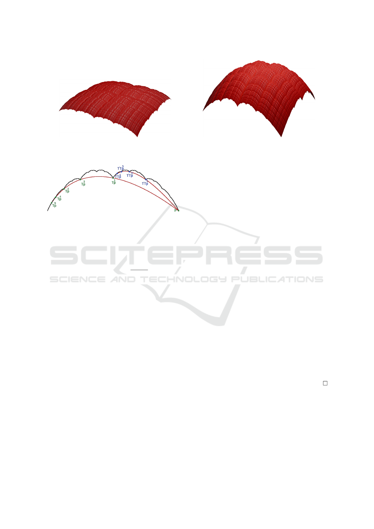
Figure 1: The attractors of two P-IFS that are the tensor product of two Takagi-like IFS. The operators of the IFS share their
second eigenvectors, but their tangent plane (defined by their first eigenvectors) changes, resulting in a similar geometry, but
a varied height amplitude.
Figure 2: A P-IFS composed of two operators (T and T
′
),
whose attractor (in black) is the Takagi curve. Two DCF in
red illustrated how the point p is transformed when applying
T
n
(in green) and T
′
T
n
(in blue). Note that the DCF with
the blue points is exactly the DCF with the green points
transformed by T
′
.
where X
i
is the coordinates of Q in the eigen basis
(V
V
V
0
,V
V
V
1
, . . . ,V
V
V
NM−1
) and A
i
=
log(|Λ
i
|)
log(|Λ
1
|)
. Note that
A
0
= 0 (thus t
A
0
= 1) and A
1
= 1; When an eigen-
value is negative, a point q will jump to a different
half-plane split by the eigenvectors. This is described
in more details in section 4.
3 SURFACE DCF
Our objective is to provide a tool to analyse the cur-
vatures of a fractal surface generated from the tensor
product of fractal curves.
Considering the results obtained on DCF (detailed
in the previous part) for a fractal surface would be
like analysing a directional derivative of the surface
(at the fixed point), which is insufficient. Moreover,
analysing all DCF that are in all directions would be
too complex and chaotic. Hence we need a parametric
representation that captures the limit behavior of the
surface locally at each fixed point.
We propose to construct a Surface Differential
Characteristic Function (SDCF) of an operator T =
T ⊗ T
′
as the tensor product of the DCF of T and T
′
.
We claim that it captures the differential properties of
the attractor at the fixed point of T and is infinitely
differentiable.
The SDCF is a bivariate function defined by :
SDCF(T , Q , s,t) = DCF(T, q, s) ⊗ DCF(T
′
, q
′
,t)
From the definition of the DCF (Janbein et al., 2024),
we obtain:
SDCF(T , Q , s,t) =
N−1
∑
i=0
N
′
−1
∑
j=0
x
i
x
′
j
v
v
v
i
⊗ v
v
v
′
j
s
α
i
t
α
′
j
An illustration of a SDCF is shown in Figure 4.
We introduce the notation D
D
D
i, j
= x
i
x
′
j
v
v
v
i
⊗ v
v
v
′
j
,
which corresponds to the variable-independent part of
the SDCF formula.
As for DCF, any point of a given SDCF SD
1
taken
as a new starting point will generate a new SDCF SD
2
that is superimposed with SD
1
, but with a different
parametrisation.
Property 3.1. The graph of the SDCF of an operator
T is invariant under the SDCF.
Proof. Let ˙q = SDCF(T , q, u, r) =
∑
N−1
i=0
∑
N
′
−1
j=0
D
D
D
i, j
u
α
i
r
α
′
j
. Given the coordinates
of ˙q in the eigenbasis: ˙x
i
= x
i
x
′
j
u
α
i
r
α
′
j
. If
we take the SDCF of T from ˙q we have:
SDCF(T , ˙q, s,t) =
∑
N−1
i=0
∑
N
′
−1
j=0
˙x
i
˙x
′
j
v
v
v
i
⊗ v
v
v
j
s
α
i
t
α
′
j
=
∑
N−1
i=0
∑
N
′
−1
j=0
x
i
x
′
j
u
α
i
r
α
′
j
v
v
v
i
⊗ v
v
v
j
s
α
i
t
α
′
j
=
∑
N−1
i=0
∑
N
′
−1
j=0
D
D
D
i, j
(us)
α
i
(rt)
α
′
j
=
SDCF(T , q, us, rt).
The following property justifies the definition of
SDCF. It states that the DCF defined from an operator
of the P-IFS of the surface (T = T ⊗ T
′
) is included
in the tensor product of the two DCF defined from T
and T
′
.
Property 3.2. The DCF of T from any point q in B
N
is an embedding of the DCF of T from q ⊗ v
v
v
′
0
, i.e.
DCF(T, q,t) ⊗ v
′
0
= DCF(T , q ⊗ v
′
0
,t).
Second Order Differential Properties of Tensor Product Fractal Surfaces
287

Figure 3: Three P-IFS (having two operators) with α
2
= 1.5 on the left, α
2
= 2 in the middle, and α
2
= 2.5 on the right. Here
only λ
2
and v
v
v
2
were changed for the left operator.
Figure 4: The attractor of a P-IFS that is the tensor product
of two P-IFS T = {T
0
, T
1
} and T
′
= {T
′
0
, T
′
1
} is represented
in wireframe (red). The DCF of T
0
and T
′
0
(having respec-
tively C
1,0
and C
0,1
as starting points) are in black. The
DCF of T
0,0
= T
0
⊗ T
′
0
having C
1,1
as starting point is rep-
resented in yellow. Finally, the SDCF of T
0,0
having C
1,1
as starting point is represented in light blue. Note that all 3
DCF are included in the SDCF.
Figure 5: A P-IFS whose attractor (in red wireframe) is the
tensor product of two Takagi curves. The minimum and
maximum SDCF are shown in light blue and green respec-
tively.
Proof. We take q a point of B
N
. q ⊗ v
′
0
refers to q
embedded in B
NM
according to v
′
0
.
DCF(T , q ⊗ v
v
v
′
0
,t) =
∑
N−1
i=0
∑
N
′
−1
j=0
x
i
x
′
j
v
v
v
i
⊗ v
v
v
′
j
t
α
i
α
′
j
.
x
′
j
is 0 except for x
′
0
= 1. Thus, we
have DCF(T , q ⊗ v
′
0
,t) =
∑
N−1
i=0
x
i
v
v
v
i
⊗ e
e
e
N
′
,0
t
α
i
≡
∑
N−1
i=0
x
i
v
v
v
i
t
α
i
= DCF(T, q,t).
The previous property is also true for v
0
⊗ q
′
.
Another strong property is that the DCF with a
starting point on a SDCF is included in the SDCF.
Property 3.3. The SDCF of T from any point q con-
tains the DCF of T from q.
Proof. SDCF(T , q,t, t) =
∑
N−1
i=0
∑
N
′
−1
j=0
D
D
D
i, j
t
α
i
t
α
′
j
=
∑
N−1
i=0
∑
N
′
−1
j=0
D
D
D
i, j
t
α
i
+α
′
j
= DCF(T , q,t)
4 TANGENT AT THE FIXED
POINT OF AN OPERATOR
Given a contractive operator T with strictly decreas-
ing eigenvalues, the eigenvector (v
v
v
1
) associated with
the second greatest eigenvalue is the pseudo-tangent
at the fixed point (Bensoudane, 2009). However, there
are special cases to consider:
• λ
1
< 0: the point q will jump from one half-plane
delimited by v
v
v
2
to the other, resulting in a range
of tangents that spans the sector delimited by v
v
v
1
to −v
v
v
1
.
• λ
2
< 0: the point q will jump from one half-plane
delimited by v
v
v
1
to the other, while still converging
along v
v
v
1
, see Figure 7.
Note that there might be a transformation with
both λ
1
< 0 and λ
2
< 0, but the attractor of an IFS
with such a transformation would be ill-suited to gen-
erate surfaces, so this case is ignored.
Figures 5 and 6 illustrate some situations that arise
for surfaces. Figure 5 showcases a minimum and
maximum SDCF while Figure 6 presents some re-
markable combination of DCF.
The pseudo-tangents at the fixed point are the
same as the pseudo-tangents defined by Bensoudane
et al. (Bensoudane, 2009) and Podkorytov et al. (Pod-
korytov, 2013).
In the case of SDCF, we have pseudo-tangent-
plane at the fixed point that contains the pseudo-
tangents of the two DCF and delimits half-spaces. If
some eigenvalues of T and T
′
are negative, the point
Q will jump from one half-space to the other.
5 CURVATURE AT FIXED
POINTS
Thanks to the SDCF, which is an analytically defined
surface, we can calculate curvatures which can then
be used to estimate pseudo-curvatures of the fractal
surface and characterise its differential behaviour at
fixed points.
For a surface F (s, t), the curvatures are computed
from the first and second fundamental forms (noted I
and II below):
GRAPP 2025 - 20th International Conference on Computer Graphics Theory and Applications
288

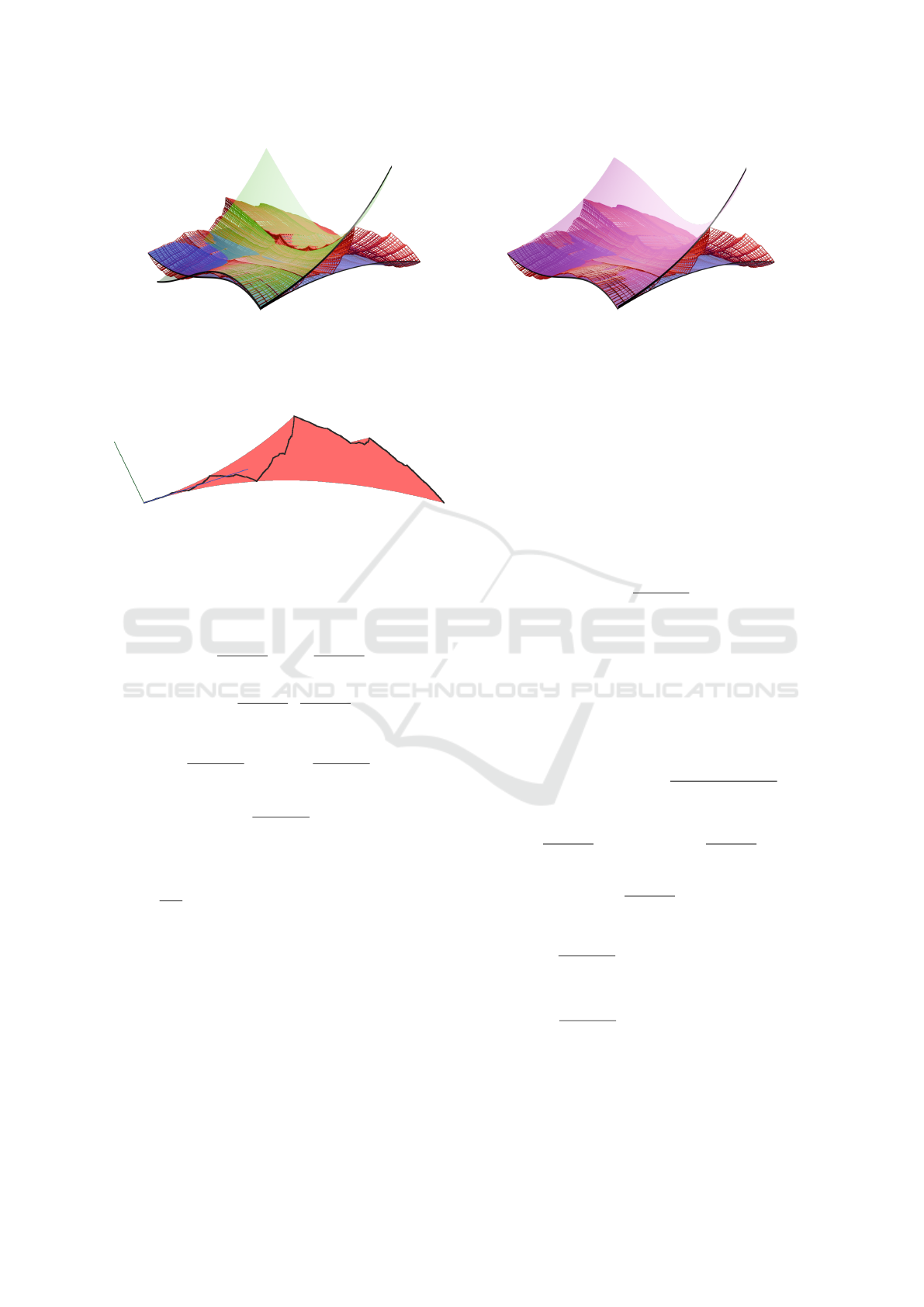
Figure 6: A P-IFS whose attractor (in red wireframe) is the tensor product of a Takagi curve and the curve in figure 7 (with a
negative λ
2
). The SDCF in blue is the tensor product of the minimum DCF of the Takagi curve and the DCF that capture the
behavior of T
n
q for even n. The SDCF in green is the tensor product of the maximum DCF of the Takagi curve and the DCF
that capture the behavior of T
n
q for odd n. The SDCF in pink is the tensor product of the minimum DCF of the Takagi curve
and the DCF that captures the behavior of T
n
q for odd n.
Figure 7: A P-IFS with λ
2
negative. Applying T
0
to a point
makes it jump from one side of v
v
v
1
(in blue) to the other.
I =

E F
F G

, II =

L M
M N

E =
∂F (s, t)
∂s
2
;G =
∂F (s, t)
∂t
2
F =
∂F (s, t)
∂s
·
∂F (s, t)
∂t
L =
∂
2
F (s, t)
∂s
2
· n
n
n
s,t
;N =
∂
2
F (s, t)
∂t
2
· n
n
n
s,t
M =
∂
2
F (s, t)
∂s∂t
· n
n
n
s,t
with n
n
n
s,t
the normal of the surface at (s,t).
For a given parametric curve f (t), we can asso-
ciate to each value of t a measure of the curvature:
κ(t) =
1
R (t)
, where R (t) is the radius of curvature at t.
For surfaces, we have the Gaussian curvature K , the
mean curvature H and the two principal curvatures
K
1
and K
2
. The Gaussian curvature K (s,t) describes
the local shape of the surface at (s,t).
• K < 0, the surface is said to have an hyperbolic
point at (s,t) and is saddle-shaped.
• K = 0, the surface is flat at (s,t) in at least a di-
rection (cylinder-like or a plane).
• K > 0, the surface is said to have an elliptic point
at (s,t) and is dome/bowl shaped.
As the SDCF approximates the fractal surface at
the fixed point, we can have an idea of the differential
behaviour of the surface by computing the curvatures
of the SDCF. The considered fixed point is the one
with s = 0 and t = 0, so it is necessary to study the
limit of the curvature of the SDCF when (s,t) goes to
(0, 0). K is defined using the first and second funda-
mental forms as:
K =
LN − M
2
EG − F
2
Since the attractor is built as an iterative process
of transformations, if we know a property at the fixed
point, we can compute it on any dyadic point of the
attractor. That’s why we first study and compute the
curvature at the fixed point: we compute the limit of
the curvature as we approach the fixed point. We ab-
breviate SDCF(T , Q , s,t) as F (s,t).
lim
(s,t)→(0,0)
n
n
n
s,t
= n
n
n
0,0
=
PD
D
D
1,0
× PD
D
D
0,1
||PD
D
D
1,0
× PD
D
D
0,1
||
lim
(s,t)→(0,0)
∂F (s, t)
∂s
= D
D
D
1,0
; lim
(s,t)→(0,0)
∂F (s, t)
∂t
= D
D
D
0,1
lim
(s,t)→(0,0)
∂F (s, t)
∂s∂t
= D
D
D
1,1
lim
(s,t)→(0,0)
∂
2
F (s, t)
∂s
2
= lim
s→0
α
2
(α
2
− 1)D
D
D
2,0
s
α
2
−2
lim
(s,t)→(0,0)
∂
2
F (s, t)
∂t
2
= lim
t→0
α
′
2
(α
′
2
− 1)D
D
D
0,2
t
α
′
2
−2
We introduce the following notations:
K
s
(s) = Pα
2
(α
2
− 1)D
D
D
2,0
s
α
2
−2
K
t
(t) = Pα
′
2
(α
′
2
− 1)D
D
D
0,2
t
α
′
2
−2
The computation
of the limit of the Gaussian curvature of the SDCF at
Second Order Differential Properties of Tensor Product Fractal Surfaces
289

the point (0, 0) is expressed as follows:
lim
(s,t)→(0,0)
K
s
(s) · n
n
n
s,t
K
t
(t) · n
n
n
s,t
− (PD
D
D
1,1
.n
n
n
s,t
)
2
(PD
D
D
1,0
)
2
· (PD
D
D
0,1
)
2
− (PD
D
D
1,0
· PD
D
D
0,1
)
2
Note that the denominator is a constant:
(PD
1,0
)
2
(PD
0,1
)
2
− (PD
1,0
· PD
0,1
)
2
. This constant
equals 0 if (PD
1,0
)
2
· (PD
0,1
)
2
= (PD
1,0
· PD
0,1
)
2
.
From the Cauchy-Schwarz inequality, we know
that this equality holds only if PD
0,1
and PD
1,0
are
linearly dependent.
We have 3 cases for the Gaussian curvature of
each operator:
• α
2
< 2: the first term α
2
(α
2
− 1)D
D
D
2,0
s
α
2
−2
·
n
n
n
0,0
is infinite and all other terms don’t matter
(lim
s→0
s
α
i
−2
= ∞)
• α
2
= 2: the first term α
2
(α
2
− 1)D
D
D
2,0
s
α
2
−2
is a
constant and all other terms are either constant or
null.
• α
2
> 2 all terms vanish (α
i
−2 will always be pos-
itive so lim
s→0
s
α
i
−2
= 0)
Assuming we do not have the degenerate case with
linearly dependent vectors, we have 9 possibilities
when we combine the cases of K
s
and K
t
for the
Gaussian curvature:
• α
2
> 2, α
′
2
> 2: the limit of K
s
and K
t
is infinite,
so the curvature is infinite,
• α
2
> 2, α
′
2
= 2: the limit of K
s
is infinite and the
limit of K
t
is finite and non-null, so the curvature
is infinite,
• α
2
> 2, α
′
2
< 2: the limit of K
s
is infinite and the
limit of K
t
is null, so the curvature does not exist,
• α
2
= 2, α
′
2
= 2: the limit of K
s
and K
t
is fi-
nite and non-null, so the curvature is finite and is
PD
2,0
·n
n
n
0,0
PD
0,2
·n
n
n
0,0
−(PD
D
D
1,1
.n
n
n
s,t
)
2
(PD
D
D
1,0
)
2
·(PD
D
D
0,1
)
2
−(PD
D
D
1,0
·PD
D
D
0,1
)
2
,
• α
2
= 2, α
′
2
< 2: the limit of K
s
is finite and
non-null K
t
null, so the curvature is finite and is
−(PD
D
D
1,1
.n
n
n
s,t
)
2
(PD
D
D
1,0
)
2
·(PD
D
D
0,1
)
2
−(PD
D
D
1,0
·PD
D
D
0,1
)
2
• α
2
< 2, α
′
2
< 2: the limit of K
s
and K
t
is null, so the curvature is finite and is
−(PD
D
D
1,1
.n
n
n
s,t
)
2
(PD
D
D
1,0
)
2
·(PD
D
D
0,1
)
2
−(PD
D
D
1,0
·PD
D
D
0,1
)
2
.
We summarize the preceding cases in the following
table:
lim
(s,t)7→(0,0)
K α
2
< 2 α
2
= 2 α
2
> 2
α
′
2
< 2 ±∞ ±∞
/
0
α
′
2
= 2 ±∞ K K
α
′
2
> 2
/
0 K K
For the mean and principal curvatures, the calcu-
lations are carried out in the same way.
6 CURVATURE OF AN
ATTRACTOR
The computation of the curvature on a differentiable
curve gives a unique value at each point of the curve.
For nowhere differentiable curves like fractals, Jan-
bein et al. (Janbein et al., 2024) have computed
pseudo-curvatures (in the form of curvature ranges) at
each side of every dyadic points. For surfaces, where
multiple curvature metrics exist (Gaussian, Mean and
principal curvatures), we find again a range for each
of these values. Depending on the starting point, the
SDCF changes, resulting in a family of SDCF whose
volume acts as a hull to the attractor. As for nowhere
differentiable curves, where pseudo-curvatures are
first computed (in the form of curvature ranges) at
the fixed point of each operator T and then deduced
at each side of every dyadic points, the same apply
for tensor product fractal surfaces. It hence gives us
the opportunity to characterize the nature of a tensor
product fractal surface (defined by four operators) at
any dyadic point, that can be: concave/convex ellip-
soid, cylindrical, hyperboloid . . .
7 CONCLUSION
In this paper, we have extended the definition of the
pseudo-curvature from P-IFS-generated curves to ten-
sor product fractal surfaces. This was done through
the definition of the SDCF, seen as the tensor product
of the two DCF associated to the curves from which
the attractor is formed.
Taking the first derivative of a SDCF results in a
pseudo-tangent that accurately represent the first or-
der differential behavior of the attractor. The second
derivative of a SDCF yields pseudo-curvatures that
correspond to the second order differential behavior
of the surface. Unlike for smooth surfaces that have
a single value of curvature per point, we have shown
that fractal surfaces have ranges of pseudo-curvatures,
due to the intricate complexity of their geometry. The
pseudo-curvature computation is based on the anal-
ysis of their eigenvalues and eigenvectors (for each
implied operator). As a future work, we would like to
explore how the control of the second order differen-
tial behavior of the surface (via the eigen values and
vectors) can have an influence on its perceived rough-
ness. It hence would give us the opportunity to control
roughness, as shown in Figure 8.
We are also interested in studying the DCF (resp.
SDCF) of P-IFS with more than two (resp. four)
transformations. This study must take particular at-
tention to the fixed points of the non-extrema transfor-
GRAPP 2025 - 20th International Conference on Computer Graphics Theory and Applications
290

Figure 8: The attractors of two P-IFS with a similar geometry, but with widely different range of pseudo-curvature, resulting
in a different roughness.
mations. Ensuring continuity at every junction points
is not enough to guarantee continuity at every dyadic
point on such curves and surfaces. Then, we are in-
terested in the differential properties of fractals that
can be constructed using Controlled Iterated Function
System C-IFS that extends the definition of the plain
IFS or P-IFS with an automaton that decides which
operator to apply, based on the current state and its
transition rules, allowing a larger variety of possible
surfaces. Finally we would like to generalize our re-
sults to non tensor-product fractal surfaces, which is
more complex than the case of tensor product surface,
both because of the freer transformations, and the po-
tentially non-grid subdivision scheme.
ACKNOWLEDGEMENTS
This work benefited from the support of the project
Fraclettes ANR-20-CE46-0003 of the French Na-
tional Research Agency (ANR).
REFERENCES
Banach, S. (1922). Sur les op
´
erations dans les ensembles
abstraits et leur application aux
´
equations int
´
egrales.
Fundamenta Mathematicae, 3:133–181.
Barnsley, M. F. (1986). Fractal functions and interpolation.
Constructive Approximation, 2(1):303–329.
Barnsley, M. F. (1988). Fractals Everywhere. Dover Publi-
cations, Inc.
Bensoudane, H. (2009). Etude diff
´
erentielle des formes
fractales. PhD thesis, Universit
´
e de Bourgogne.
Bensoudane, H., Gentil, C., and Neveu, M. (2009). Frac-
tional half-tangent of a curve described by iterated
function systems. Journal Of Applied Functional
Analysis, 4(2).
Bigerelle, M., Nianga, J.-M., Najjar, D., Iost, A., Hubert,
C., and Kubiak, K. (2013). Roughness signature of tri-
bological contact calculated by a new method of peaks
curvature radius estimation on fractal surfaces. Tribol-
ogy International, 65:235–247.
Bolzano, B. (1950). Paradoxes of the Infinite. Rare master-
pieces of philosophy and science. Routledge and Paul.
Hutchinson, J. E. (1981). Fractals and self similarity. Indi-
ana University Mathematics Journal, 30:713–747.
Janbein, M., Gentil, C., Roudet, C., and Poull, C. (2024).
Pseudo-curvature of fractal curves for geometric con-
trol of roughness. In 19th International Conference
on Computer Graphics Theory and Applications, vol-
ume 1 of GRAPP, HUCAPP and IVAPP, pages 177–
188, Rome, Italy.
Lindenmayer, A. (1968). Mathematical models for cellular
interactions in development ii. simple and branching
filaments with two-sided inputs. Journal of Theoreti-
cal Biology, 18(3):300–315.
Podkorytov, S. (2013). Espaces tangents pour les formes
auto-similaires. PhD thesis, Universit
´
e de Bourgogne.
Podkorytov, S., Gentil, C., Sokolov, D., and Lanquetin, S.
(2013). Geometry control of the junction between two
fractal curves. Computer-Aided Design, 45(2):424–
431.
Podkorytov, S., Gentil, C., Sokolov, D., and Lanquetin, S.
(2014). Joining primal/dual subdivision surfaces. In
Mathematical Methods for Curves and Surfaces: 8th
International Conference, MMCS 2012, Oslo, Nor-
way, June 28–July 3, 2012, Revised Selected Papers
8, pages 403–424. Springer.
Takagi, T. (1901). A simple example of the contin-
uous function without derivative. Tokyo Sugaku-
Butsurigakkwai Hokoku, 1:F176–F177.
Zair, C. E. (1998). Formes fractales
`
a p
ˆ
oles bas
´
ees sur une
g
´
en
´
eralisation des IFS. PhD thesis, PhD thesis, Uni-
versit
´
e Claude Bernard-LYON-1.
Zair, C. E. and Tosan, E. (1996). Fractal modeling using
free form techniques. In Computer Graphics Forum,
volume 15, pages 269–278. Wiley Online Library.
Second Order Differential Properties of Tensor Product Fractal Surfaces
291