Single-Exemplar Lighting Style Transfer via

Emissive Texture Synthesis and Optimization

Pierre Ecormier-Nocca

, Lukas Lipp

, Annalena Ulschmid

, David Hahn

and Michael Wimmer

Institute of Visual Computing and Human-Centered Technology, TU Wien, Vienna, Austria

Keywords:

Lighting Design, Lighting Style Ttransfer, Texture Synthesis, Lighting Optimization.

Abstract:

Lighting is a key component in how scenes are perceived. However, many interior lighting situations are

currently either handcrafted by expert designers, or simply consist of basic regular arrangements of luminaires,

such as to reach uniform lighting at a predeﬁned brightness. Our method aims to bring more interesting

lighting conﬁgurations to various scenes in a semi-automatic manner designed for fast prototyping by non-

expert users. Starting from a single photograph of a lighting conﬁguration, we allow users to quickly copy

and adapt a lighting style to any 3D scene. Combining image analysis, texture synthesis, and light parameter

optimization, we produce a lighting design for the target 3D scene matching the input image. We validate via

a user study that our results successfully transfer the desired lighting style more accurately and realistically

than state-of-the-art generic style transfer methods. Furthermore, we investigate the behaviour of our method

under potential alternative choices in an ablation study.

1 INTRODUCTION

Lighting design is often overlooked in the early phase

of architectural planning, or requires expert knowl-

edge for speciﬁc design tasks. While common con-

struction projects apply simple, well-known solutions

to achieve regulatory compliance, the available design

space is rarely explored further. Even then, manually

arranging complex lighting setups for interior design

is a laborious task. We instead envision a workﬂow

that allows non-expert users to create lighting designs

for a target scene using a copy-and-paste metaphor.

In this paper we establish a user-controllable,

semi-automatic pipeline, allowing the user to capture

lighting conditions of a single reference image, and

then transfer them to the target scene. Existing meth-

ods for image-based style transfer, however, are not

sufﬁcient to achieve this goal, as they ignore the geo-

metric structure of the 3D target scene and the physics

of light transport. We, instead, ﬁrst extract light-

ing information from the exemplar image in a user-

https://orcid.org/0000-0002-3975-4913

https://orcid.org/0000-0002-1110-0707

https://orcid.org/0000-0002-0539-9378

https://orcid.org/0000-0002-7617-5523

https://orcid.org/0000-0002-9370-2663

guided segmentation step, correct for distortion in the

input using perspective and vanishing point analysis,

and then synthesize an emissive texture for the target

scene. Finally, we optimize the colour cast and inten-

sity of the emissive texture to correct for indirect il-

lumination effects in the target scene using an inverse

rendering approach. In this way, we transfer the light-

ing style while keeping user interactions to a mini-

mum, but still enabling a controllable copy-and-paste

user experience. We show results of our system on

various indoor scenes and style exemplars. In a user

study we demonstrate clear advantages over state-of-

the-art image style transfer methods. Note that our re-

sults are not simply modiﬁed images, but physically-

based renderings of the modiﬁed 3D scenes taking

global illumination into account. Overall, our ap-

proach, illustrated in Fig. 1, opens the lighting design

space to non-expert users. Our results rely on the fol-

lowing scientiﬁc contributions:

• An efﬁcient data-augmented method for semi-

automatic segmentation (§4) and annotation of

photographs,

• an automatic texture unwarping and perspective

correction method for indoor images (§5),

• and an emissive texture synthesis and lighting op-

timization routine (§6).

Ecormier-Nocca, P., Lipp, L., Ulschmid, A., Hahn, D. and Wimmer, M.

Single-Exemplar Lighting Style Transfer via Emissive Texture Synthesis and Optimization.

DOI: 10.5220/0013193900003912

Paper published under CC license (CC BY-NC-ND 4.0)

In Proceedings of the 20th International Joint Conference on Computer Vision, Imaging and Computer Graphics Theory and Applications (VISIGRAPP 2025) - Volume 1: GRAPP, HUCAPP

and IVAPP, pages 113-126

ISBN: 978-989-758-728-3; ISSN: 2184-4321

113

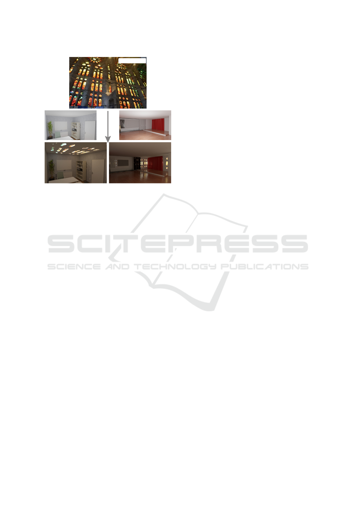
Style Exemplar

Style Transfer

Lighting

Figure 1: We transfer the lighting setup from a single input

image to any 3D scene by extracting a perspective-corrected

light mask via data-guided segmentation. We generate an

emissive texture from the extracted light mask and apply it

to the 3D scene. We then optimize its emissive parameters

to match the colour of the input image.

2 PREVIOUS WORK

Lighting design typically involves manually plac-

ing light ﬁxtures and verifying regulatory compli-

ance with industry-standard software tools (DIAL

GmbH, 2022; Relux Informatik AG, 2022), which

is a time-consuming process. Consequently, simple

arrays of lights are ubiquitous solutions. Computa-

tional lighting design has been explored based on user

hints (Schoeneman et al., 1993; Anrys et al., 2004;

Pellacini et al., 2007; Okabe et al., 2007; Lin et al.,

2013), procedural modeling and optimization (Kawai

et al., 1993; Schwarz and Wonka, 2014; Gkaravelis,

2016; Jin and Lee, 2019), or visualization and sugges-

tive design (Sorger et al., 2016; Walch et al., 2019).

While these methods provide more approachable so-

lutions to lighting design, they still require user exper-

tise to produce the expected results. As we target both

expert and novice users, we formulate our method

around a straightforward pipeline that requires no pre-

vious knowledge of lighting design. Recent methods

also propose data-driven neural scene lighting (Ren

et al., 2023), focusing on automatic generation of

lighting designs based on a sufﬁciently large training

data set. In contrast, we pursue a user-directed single-

input style transfer approach.

Texture synthesis has been widely explored in

Computer Graphics, producing a large variety of ap-

proaches. Starting from pixel-based methods (Efros

and Leung, 1999; Tong et al., 2002), the ﬁeld has

evolved to patch-based (Efros and Freeman, 2001;

Kwatra et al., 2003) and optimization-based (Kwa-

tra et al., 2005) methods, and recently to deep neural

networks and generative adversarial networks (Sendik

and Cohen-Or, 2017; Fr

uhst

uck et al., 2019; Zhou

et al., 2018b). These methods usually assume a con-

trolled input, meaning a high quality image of an

undistorted albedo texture, without lighting or noise,

although some can be adapted to different input con-

ditions. We use texture synthesis for lighting conﬁgu-

rations, which is an unusual application with speciﬁc

challenges. Neural methods in particular would need

to be explicitly trained on textures of lighting setups

to produce coherent results. We therefore opt for more

traditional techniques and adapt them to tackle the

speciﬁc challenges of lighting texture synthesis in §6.

A few methods handle texture synthesis from un-

controlled images (Eisenacher et al., 2008; Diamanti

et al., 2015), but they operate on a different set of as-

sumptions, making them unsuitable for lighting de-

sign. For example, they might require manual seg-

mentation of the texture, which in our case could cor-

respond to a large number of small light sources, mak-

ing it unnecessarily tedious for the user. They also

require manually annotating the geometry, which is

time consuming, and operating with pixel-based syn-

thesis is only practical for dense textures.

Neural style transfer copies the artistic style from

one image to another. After its introduction (Gatys

et al., 2015), neural style transfer has seen multiple

improvements over the years, with developments spe-

ciﬁc to many different applications (see (Jing et al.,

2018) for an overview). In particular, (Li et al.,

2018) present a method for photorealistic style trans-

fer, which can also transfer lighting from image to im-

age. However, as these approaches only work on im-

ages instead of the actual lighting of a 3D scene, there

is no physical plausibility to the transfer, leading to

unexpected and undesirable results. We instead focus

on predictable and physically based lighting, produc-

ing a 3D scene as output instead of an image.

Lighting optimization has been made possible by

inverse rendering methods, where light source param-

eters can be optimized efﬁciently via differentiable

rendering (Zhang et al., 2020; Jakob et al., 2022; Lipp

et al., 2024). While these methods are physically ac-

curate, they can be difﬁcult to conﬁgure to get the de-

sired results, as the user needs to specify a suitable

target illumination for the scene. Instead, we aim to

bridge the gap between manual lighting design and

fully automated optimization by providing a plausible

ﬁrst solution of the design, which could then be fur-

GRAPP 2025 - 20th International Conference on Computer Graphics Theory and Applications

114

Input

Perspective

Analysis

Rendering

Data Extraction Segmentation Synthesis

Texture

Unwarping

Optimization

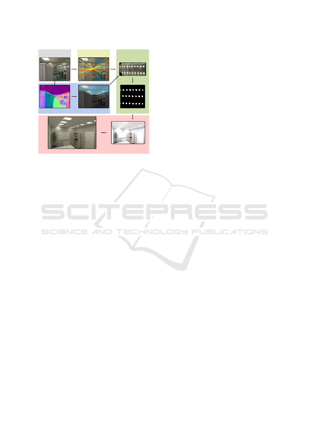
Figure 2: Overview of the lighting transfer pipeline. Se-

mantic data is extracted from the original input image to

assist the user-guided segmentation process. Simultane-

ously, we analyze the input image’s vanishing points to later

allow for perspective corrections. Both serve as input to

the texture synthesis procedure. Based on the perspective-

corrected light mask, we construct an unwarped emissive

texture, which we apply to a surface in the 3D scene. Lastly,

we optimize the lighting parameters to match the input im-

age following the approach of (Lipp et al., 2024).

ther ﬁne-tuned if needed by more speciﬁc optimiza-

tion methods.

3 OVERVIEW

In this paper, we consider the following problem:

given an input image showing visible light sources,

can we modify an arbitrary 3D scene to mimic the

mood and perception of the input example by only

editing the lighting of the scene? As additional con-

straints, we aim to produce physically plausible light-

ing to enable realization of our designs. We also con-

sider non-expert users in formulating our method.

As exactly reproducing the input lighting condi-

tions is typically not possible, we extract important

information on the lighting style from a single input

image. We focus on the actual light sources visible in

the image, delivering information on the size, shape,

colour and arrangement of lights. We then aim to

recreate light sources similar to the input image and

integrate them into the output 3D scenes.

Note that light sources visible in the input are of-

ten distorted by perspective and might be too close or

too spread out for the target scene, so directly copying

this data is not possible. Even if the light sources were

copied to the 3D scene, there is no guarantee that the

resulting lighting will produce a similar effect to the

input image, as light will be affected differently by

various materials throughout the scene.

3.1 Constraints and Context

We design our method for minimal user requirements,

while providing an interactive workﬂow and allowing

for artistic expression. We choose to operate on single

images of a lighting installation, allowing users to se-

lect virtually any available image, possibly captured

with low-quality devices. As a result, our method is

built to be robust against reasonable amounts of noise

and low resolutions, and does not rely on any addi-

tional data sources or training data. We ask the user to

provide system-assisted annotations in the reference

image, which both gives more freedom to the user and

more accurately delivers the expected result.

We operate on a set of assumptions speciﬁc to the

use case of interior lighting design, allowing us to in-

ject information into our model and as a result keep

the input requirements as low as possible. First, we

expect the input images to be of building interiors,

which implies closed spaces and controlled lighting.

Second, we only work with planar surfaces, as they

constitute the majority of interiors. Finally, we also

expect low-distortion rectilinear images, thus exclud-

ing ﬁsheye lenses or similarly distorted perspectives.

3.2 Pipeline

As illustrated in Fig. 2, we start by extracting seman-

tic data from a single RGB image, including depth,

3D positions and normals. This information is ag-

gregated as high-dimensional vectors per pixel and

employed to assist the user in providing a meaning-

ful segmentation of the image. We then ask the user

to delimit the plane containing the lighting ﬁxtures

of interest, and to delineate (a subset of) lights that

should be transferred. We then estimate the perspec-

tive transform using image processing techniques and

optimization of the vanishing points in Hough space,

resulting in the coordinates of the image’s vanishing

points in all three dimensions (even if some vanishing

points lie at inﬁnity). We use this data to correct the

perspective of the selected lighting setup.

Applying this perspective correction to the user-

selected lighting conﬁguration produces an “un-

warped” lighting image, which we use as input for

texture synthesis. In this way, we generate arbitrarily

large replica of the image’s lighting features, which

we apply to the target 3D scene as an emissive texture

on a user-selected surface. Finally, we optimize the

intensity and colour of the emissive texture using a

Single-Exemplar Lighting Style Transfer via Emissive Texture Synthesis and Optimization

115

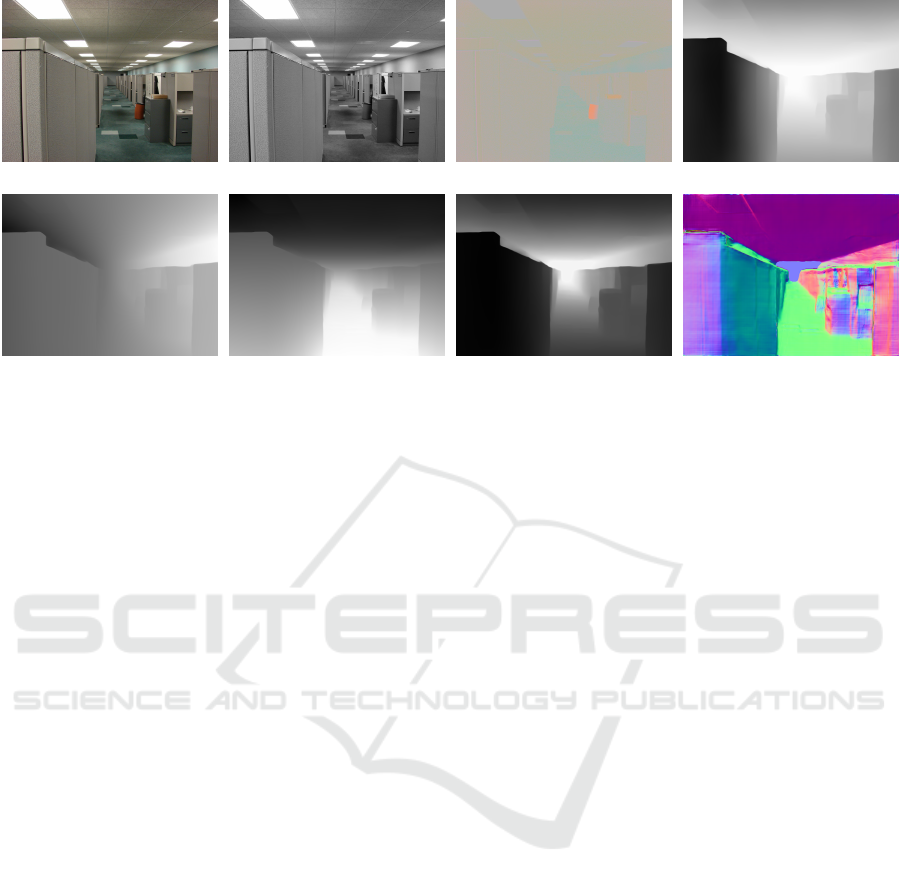
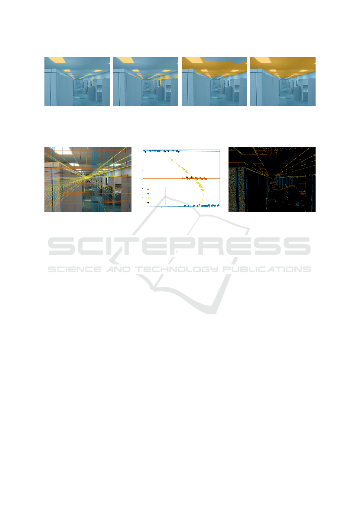
(a) Original image (b) CIELAB lightness (c) CIELAB colour (d) Depth

(e) X coord. (world-space) (f) Y coord. (world-space) (g) Z coord. (world-space) (h) Normals

Figure 3: Extracted information from the input image used to guide the segmentation. These additional data channels provide

semantic information to the system, allowing a ﬁner segmentation of the input. From the original image (a), we convert to

CIELAB colour space (b,c) and estimate depth (d) using MiDaS (Ranftl et al., 2022). The depth is then used to estimate

world-space coordinates (e, f, g) and normals (h). See also Fig. 6 on how this data affects segmentation behaviour.

view-independent inverse rendering framework (Lipp

et al., 2024), such that the light reﬂected back from

the 3D scene onto the textured surface matches the

ambient colour of the original input image.

4 DATA-GUIDED FEATURE

SELECTION

In this section, we discuss our analysis of the input

image, before moving on to perspective correction,

and lighting optimization.

4.1 Data Extraction

Given an input image, we ﬁrst extract contextual and

semantic information for each pixel, which we then

use for data-guided segmentation. All the aggregated

data is represented in Fig. 3. First, we estimate the im-

age depth using the deep neural network MiDaS (Ran-

ftl et al., 2022), designed for robust monocular depth

estimation. As we use depth only to provide addi-

tional information for segmentation, we do not re-

quire highly accurate results. Similarly, one could

capture a 2.5D input image using a RGB-D camera.

Next, we estimate 3D coordinates based on the es-

timated depth per pixel by inverting a standard pro-

jection matrix. We use the common projection matrix

P(t,b,l,r, f , n) of a frustum with bounds t, b,l,r at the

top, bottom, left, and right, as well as far and near

plane distances f and n. As we are only looking for a

rough estimate for the 3D coordinates, we choose val-

ues of (−1; 1) for the left-right and bottom-top pairs,

and (1; 10) for the near and far planes. Note that we

do not require the precise values for the input im-

age, as the projection is normalization invariant. The

world-space coordinates p

= (x

) of each

pixel then follow from the screen-space 2.5D location

and depth of the pixel p

= (x

) as:

= P

−1

. (1)

Furthermore, we use Open3D (Zhou et al., 2018a)

to estimate normals from nearest neighbours within

the resulting world-space point cloud. Once again,

obtaining ground truth normals is not necessary,

as long as the normals are consistent and accurate

enough to infer semantic meaning. Finally, we con-

vert the RGB data to the CIELAB colour space, pro-

ducing one channel for lightness and two channels for

perceptually uniform colour data. While the guided

segmentation procedure could operate in RGB or

other colour spaces, we utilize CIELAB to more ac-

curately represent user intent, which is usually based

on brightness or colour similarity.

4.2 Guided Segmentation

Our pipeline provides the user with a semi-automatic,

data-guided image-segmentation interface. In this in-

terface, they can paint on parts of the image to sep-

arate regions corresponding to the objects of inter-

est from the background. Usually, only a few clicks

are necessary to produce an accurate segmentation of

the image. The segmentation process consists of two

phases: in the ﬁrst step, the user delineates a plane

GRAPP 2025 - 20th International Conference on Computer Graphics Theory and Applications

116

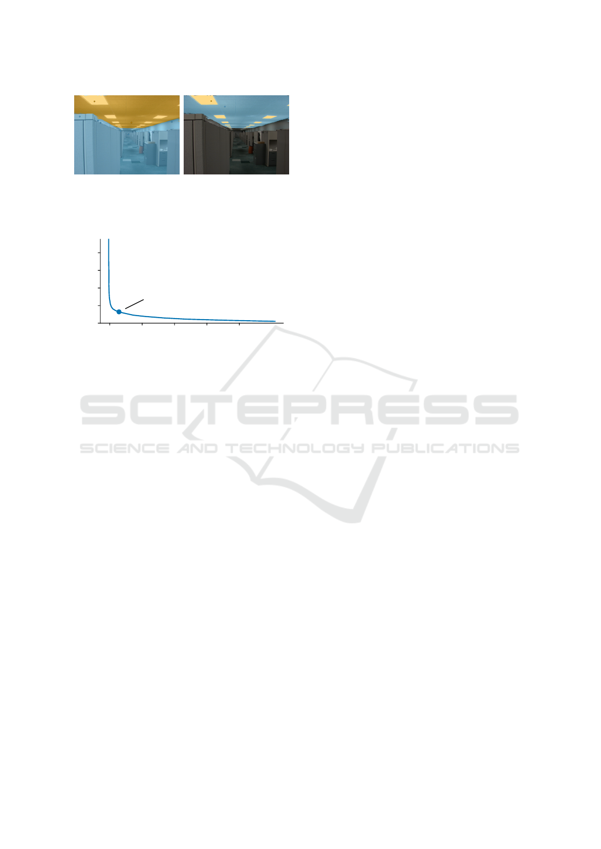
Figure 4: Two-step guided segmentation: First, the plane on

which the lights lie is identiﬁed (left). Then, the individual

lights within the plane are selected (right). Orange indicates

selected regions (positive), while blue represents culled re-

gions (negative).

0.2 0.6 1.0

Time [s]

Error

1000 samples/class

err = 1.3%

time = 0.257s

Figure 5: Evolution of the computation time and segmenta-

tion error as the number of samples per class increases from

5 to 25k.

containing the lighting setup (Fig. 4, left), and in the

second step selects the actual lights within this plane

(Fig. 4, right).

We segment the image by interpreting the user’s

annotations as positive and negative examples of a bi-

nary classiﬁer. To reduce training time, while keep-

ing a statistically similar pixel distribution, we ran-

domly sample up to a thousand pixels per class. In

this way, we achieve interactive frame rates during

the selection process. Figure 5 shows the evolution of

the segmentation error and computation time based on

the number of samples used for each class. We mea-

sure the segmentation error as intersection over union

(IoU) compared to the reference using all available

samples. The computation time includes both training

and inference over the whole image, and the number

of samples per class increases from 5 to 25k, which is

slightly less than the total available. The ﬁgure shows

that choosing 1000 samples per class results in an er-

ror of around 1.3% in this case, and keeps the total

runtime around 250 ms regardless of the number of

user annotations. We use the same number of samples

in all our results, as it provides a good speed vs. accu-

racy trade-off in general.

For each of the selected samples, we use the previ-

ously extracted data to compute the likelihood of that

pixel being selected or not. Utilizing the extracted

data is one of the central aspects of our method, al-

lowing semantic, and thus faster and more intuitive

segmentation of the input image. For example, se-

lecting the ceiling of a room is implicitly captured by

the model as selecting pixels where the normal points

down and can be differentiated from other down-

facing surfaces based on the y coordinate. In Fig. 6

we show an ablation study, where we use the same

set of inputs to segment the image with different sub-

sets of the extracted data. While using only a subset

results in undesired behaviour, with the full extracted

data available, the ceiling is successfully segmented.

5 PERSPECTIVE CORRECTION

Although the quality of the depth estimation we have

employed earlier is sufﬁcient to gain some 3D infor-

mation for classiﬁcation purposes, it is far from ac-

curate enough to model the perspective visible in the

image. In order to produce an undistorted emissive

texture, we now focus on improving the perspective

correction with an automated method based on the

Hough transform and vanishing point estimation. Our

approach achieves highly accurate perspective cor-

rection, which prevents propagating projection errors

and artifacts into later stages of the pipeline.

Vanishing point estimation has been studied

in Computer Vision since the beginning of the

ﬁeld (Magee and Aggarwal, 1984) and improved ever

since. More recent methods use the Hough trans-

form (Chen et al., 2010; Wu et al., 2021) or neural net-

works (Liu et al., 2021). Here, we describe an alter-

native formulation based on RANSAC and the Hough

transform, and in particular, a specially tailored met-

ric necessary for our vanishing point optimization.

5.1 Hough Transform for Line

Detection

The Hough transform (Duda and Hart, 1972) is a

well established method for line detection. Every line

can be uniquely represented by the polar coordinates

(ρ,θ) of the point on the line closest to the origin.

After running the standard Canny edge detection al-

gorithm (Canny, 1986) on the input image, every pos-

sible line passing through each detected edge point

is saved to an accumulator in its polar representation.

The local maxima of this accumulator correspond to

the most prominent lines in the image. However, the

main drawback of this approach is that all aligned

points sitting on an edge will be registered as a line,

which in the case of noise will produce many false

positives. To alleviate this issue, we instead compute

the image-space gradients G

and G

, and the gra-

dient direction θ

= arctan 2(G

). We then only

(in our case

Single-Exemplar Lighting Style Transfer via Emissive Texture Synthesis and Optimization

117

(a) LAB (b) LAB + D (c) LAB + D + XYZ (d) LAB + D + XYZ + N

Figure 6: Ablation study for segmentation of the input image: extracting the ceiling given the same user inputs, guided by

different subsets of the available data. Using only colour (a), or colour and depth (b) focuses too much on the bright areas

and fails to select a coherent surface; adding spatial coordinates (c) and also estimated normals (d) substantially improves the

segmentation. In this way, we achieve an intuitive interaction with very sparse user inputs.

(a)

-500 0

500 1000

X dim.

Y dim.

Z dim.

Outlier

(b) (c)

Figure 7: Vanishing point optimization: Lines are extracted from the input image using a gradient-restricted Hough transform

and displayed colour-coded per dimension (a). The points in Hough space corresponding to these image-space lines are

successively classiﬁed, whereby the ﬁtted lines correspond to the three vanishing points (b). The image edges are then

coloured by the closest corresponding dimension (c).

±2.5

◦

) to the accumulator. This signiﬁcantly helps

to reduce false positives and improves computation

speed. The resulting Hough space after maxima ex-

traction is shown in Fig. 7b.

5.2 Finding Vanishing Points

As explained in the previous section, lines in image-

space are represented with polar coordinates as points

in Hough space. Conversely, image-space points can

be represented in Hough space as the curve of all

image-space lines passing through the point. As a re-

sult, it is possible to ﬁnd the main vanishing points,

deﬁning the perspective of an input image, by ﬁnd-

ing valid curves in Hough space corresponding to the

intersection of many image-space lines.

Due to noise in the reference image, as well as un-

certainty in the line detection process, the extracted

lines do not uniquely deﬁne a vanishing point. There-

fore, an optimization procedure is required to ﬁnd the

most likely location of each vanishing point. In most

images at least one, often multiple, of the vanishing

points lie outside the image boundaries, often near in-

ﬁnity. To allow the optimization process to ﬁnd van-

ishing points both inside the image boundaries and at

inﬁnity, we express the optimized vanishing point in

polar coordinates (ρ

,θ

) and map ρ

to another vari-

able α

deﬁned as α

= 1 −1/(ρ

+ 1). This maps the

original [0;+∞[ range of ρ

to a bounded [0;1] range,

which can be fully explored during the optimization.

Optimization techniques rely on a loss metric to

point them in the direction of a locally optimal so-

lution. To measure how well a given vanishing point

matches the lines present in the original image, we ad-

ditionally develop a novel point-line metric. Indeed,

naive approaches to this problem are not suitable to

the case of vanishing points and thus do not allow

convergence. For example, considering the Euclidean

distance between the lines and point in Hough space

does not yield consistent results: as a consequence of

representing image-space lines as polar coordinates,

the Hough space is composed of distances on one axis

and angles on the other, which are not easily compa-

rable. Similarly, while considering only the point-line

distance in image-space works for vanishing points

situated within the image, this approach fails when

the vanishing point is located outside the image or at

inﬁnity. Indeed, a vanishing point at inﬁnity should be

considered to perfectly match all parallel lines in the

direction of this point. However, the standard point-

line distance does not decrease when the point moves

to inﬁnity, but remains constant (Fig. 8c). Thus it is

GRAPP 2025 - 20th International Conference on Computer Graphics Theory and Applications

118





















Image

boundary





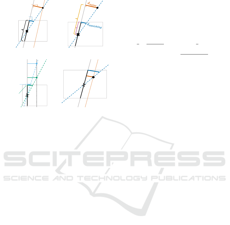
(a) Notation

𝑃

𝑥

𝑦

Image boundary

𝐶

(b) Ratio Calculation

𝑑

𝑛𝑎𝑖𝑣𝑒

𝑑

𝑛𝑎𝑖𝑣𝑒

𝑑

𝑣𝑎𝑛𝑖𝑠ℎ𝑖𝑛𝑔

𝑑

𝑣𝑎𝑛𝑖𝑠ℎ𝑖𝑛𝑔

𝑃

Image

boundary

moving towards inﬁnity

Image

boundary

𝑃

𝑑

𝑣𝑎𝑛𝑖𝑠ℎ𝑖𝑛𝑔

𝑑

𝑛𝑎𝑖𝑣𝑒

(d) Vanishing point inside

the image boundaries

Figure 8: Vanishing point metric calculated by applying

Thales’ theorem and weighting d

naive

with the ratio x/y de-

picted in (b). As can be seen in (c), opposite to the naive

point-line metric, which stays constant for a vanishing point

moving towards inﬁnity (d

naive

= d

naive

), it decreases when

moving P along l

naive

vanishing

> d

vanishing

). In case P is

inside the image boundaries, we fall back to d

naive

, which is

then smaller than d

vanishing

(d).

unsuitable for vanishing point optimization.

Instead, we propose the following vanishing point

metric: deﬁne the point and line for which we want

to compute the distance as P and l, respectively (see

Fig. 8a). We construct an additional line l

vanishing

passing through P and intersecting the centre C of the

segment s of l, which is limited by the two intersec-

tions between l and the image boundaries (i.e. only

the part of l visible in the image). In practice, l

vanishing

is the line of arbitrary angle that most closely matches

l for the pixels visible in the image. For the sake of

comparison, we can deﬁne l

naive

as parallel to l and

passing through P, which represents the naive point-

line distance: the distance d

naive

between l

naive

and l

is the same as the distance between P and l. To com-

pute a distance d

vanishing

between l

vanishing

and l, we

use the distance between l

vanishing

and the endpoint of

s closest to P. Our vanishing point metric is ﬁnally de-

ﬁned as min(d

naive

, d

vanishing

). In practice, this means

that our metric is equivalent to the naive point-line

distance while the vanishing point lies roughly within

the image (see Fig. 8d), and then decreases to 0 as the

vanishing point goes to inﬁnity in a direction parallel

to l, even if P does not lie directly on l (see Fig. 8c).

To efﬁciently compute our proposed vanishing

point metric, we apply Thales’ theorem as illustrated

in Fig. 8b. We weight the naive point-line distance

with the ratio between the distance x from the center

C to the endpoint of s closest to P and the distance y

from C to the point on l closest to P:

vanishing

naive

⇒ d

vanishing

· d

naive

, (2)

where x = 0.5 · |s| and y =

|PC|

− d

naive

We use a custom regressor to optimize the best-

ﬁtting vanishing point given a set of lines in the in-

put image. Thanks to our vanishing point metric, we

match vanishing points both inside the image and at

inﬁnity, and can compute the overall minimized error

after optimization. In order to extract the three van-

ishing points corresponding to the three dimensions

visible in the image, we use the RANSAC algorithm

to successively ﬁnd groups of lines that converge in a

vanishing point. The algorithm then iterates over the

remaining lines until three vanishing points are found,

as illustrated in Fig. 7. Note that two of the vanish-

ing points, corresponding to the x dimension (orange)

and y dimension (blue), are located at inﬁnity. Con-

sequently, they have (approximately) a unique angle

θ, but are deﬁned for all distances ρ. In contrast, the

vanishing point for the z dimension (yellow) is located

inside the image, and is deﬁned for all angles θ.

5.3 Texture Unwarping

Once the perspective of the image and the three

vanishing points are known, we use this informa-

tion to correct the perspective distortion of the user-

segmented plane containing the lighting setup, recov-

ering the original geometry of the light sources. This

process ﬁrst establishes a mapping between the input

image and the undistorted space by determining the

two most important dimensions to which lines of the

user-selected region most likely belong. For each of

these two dimensions, we compute the angle of the

line from its corresponding vanishing point to every

pixel. Then, the four corners of an arbitrary axis-

aligned rectangle are selected in undistorted space and

matched to the largest quadrilateral where each pair

of sides has the same angle to one of the selected van-

ishing points. Next, we compute the homography cor-

responding to the transformation between the image-

space quadrilateral and the undistorted-space rectan-

gle. This transform is then applied to the surface se-

lected by the user in order to correct the perspective

of the original image (see Fig. 9).

Single-Exemplar Lighting Style Transfer via Emissive Texture Synthesis and Optimization

119

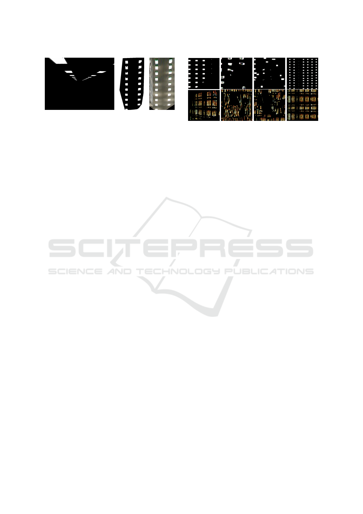
Figure 9: Texture perspective correction. Left: light mask

in the original image space. Middle: perspective-corrected

light mask. Right: corresponding undistorted zone in the

original image.

6 TEXTURE SYNTHESIS

Once the selected lighting installation has been un-

warped, we use the resulting texture as input of an

example-based texture synthesis algorithm. This step

is important since the target 3D scene can be arbi-

trarily large and as a result require arbitrarily large

textures. In our case, we operate on masked images

of light sources which are often organized follow-

ing very speciﬁc patterns. For this reason, modern

deep-learning-based texture synthesis methods would

need to be trained explicitly on data sets of light

source conﬁgurations to produce acceptable results.

Instead, in order to guarantee consistent and explain-

able results, we develop our synthesis process bor-

rowing from patch-based methods (Efros and Free-

man, 2001) and the metadata encoding from (Lefeb-

vre and Hoppe, 2005; Lefebvre and Hoppe, 2006).

Most texture synthesis algorithms, especially

pixel-based and patch-based ones, use local informa-

tion in the decision process throughout the algorithm.

This is designed for “dense” textures, where local in-

formation is abundant to optimally choose the neigh-

bouring pixels and patches. In our case of light source

synthesis, where a mask of potentially faraway lights

needs to be generated, there can be large regions of

empty space with no local information available. In

this situation, the algorithm can be ﬁne-tuned to look

for information further away. For patch-based algo-

rithms, this is modelled by the patch size. As Fig. 11

(top row) shows, choosing the right patch size can

drastically change the quality of the result.

To avoid this parameter tweaking, we instead en-

code local information about the texture directly in the

image, in the form of three additional metadata chan-

nels, similar to the approach in (Lefebvre and Hoppe,

2006). To this end, we encode local spatial informa-

tion (horizontal and vertical distance to the nearest

feature), as well as the conﬁdence of the segmentation

model for each pixel as additional distinction between

light sources and background. This additional infor-

(a) Input (b) Risser (c) Heitz et al. (d) Ours

Figure 10: Texture synthesis comparison with recent work:

(b) (Risser, 2020), (c) (Heitz et al., 2021). Due to the spe-

ciﬁc attributes of the inputs (importance of negative space,

regularity, missing information), generic synthesis algo-

rithms struggle to provide convincing results.

mation improves spatial coherence in the synthesized

texture. As demonstrated in Fig. 11 (bottom row), this

drastically improves the robustness of the synthesis

algorithm. Indeed, every block size above 25 pix-

els produces high-quality results, and the results are

much more consistent compared to direct synthesis.

Figure 12 summarizes the inputs and outputs of

our texture synthesis. Starting from the unwarped im-

age with the original colours (12a) and its metadata

(12b), we deﬁne the input as a masked emissive tex-

ture (12c), where only the light sources are visible.

During synthesis, the input is heavily downsized to

reduce computation times as shown in Fig. 12d. From

this input, the new texture’s colour (12e) and metadata

(12f) are synthesized using an iterative patch-based

approach. The resulting emissive texture is computed

by masking the output using the corresponding gener-

ated metadata, which produces Fig. 12g. As the work-

ing resolution of the generated texture is too low to

be used for rendering purposes, we then upscale the

output texture using information from the original ex-

ample image: for each generated patch, we invert the

transform for this speciﬁc patch in the unwarped im-

age, and recover the coordinates of the patch in the

original image. The full-resolution patch is then un-

warped again and added to the ﬁnal emissive texture,

resulting in a high quality texture visible in Fig. 12h.

Figure 10 shows the difference between our re-

sults and two recent methods. As the ﬁgure shows,

the strong regularity, the presence of missing regions

due to unwarping an incomplete image, and the cen-

tral role of negative space, all make generic synthesis

algorithms ill-suited to our speciﬁc use-case. In con-

trast, our method puts special care on handling miss-

ing and negative space, which produces a more accu-

rate recreation of the input examples.

GRAPP 2025 - 20th International Conference on Computer Graphics Theory and Applications

120

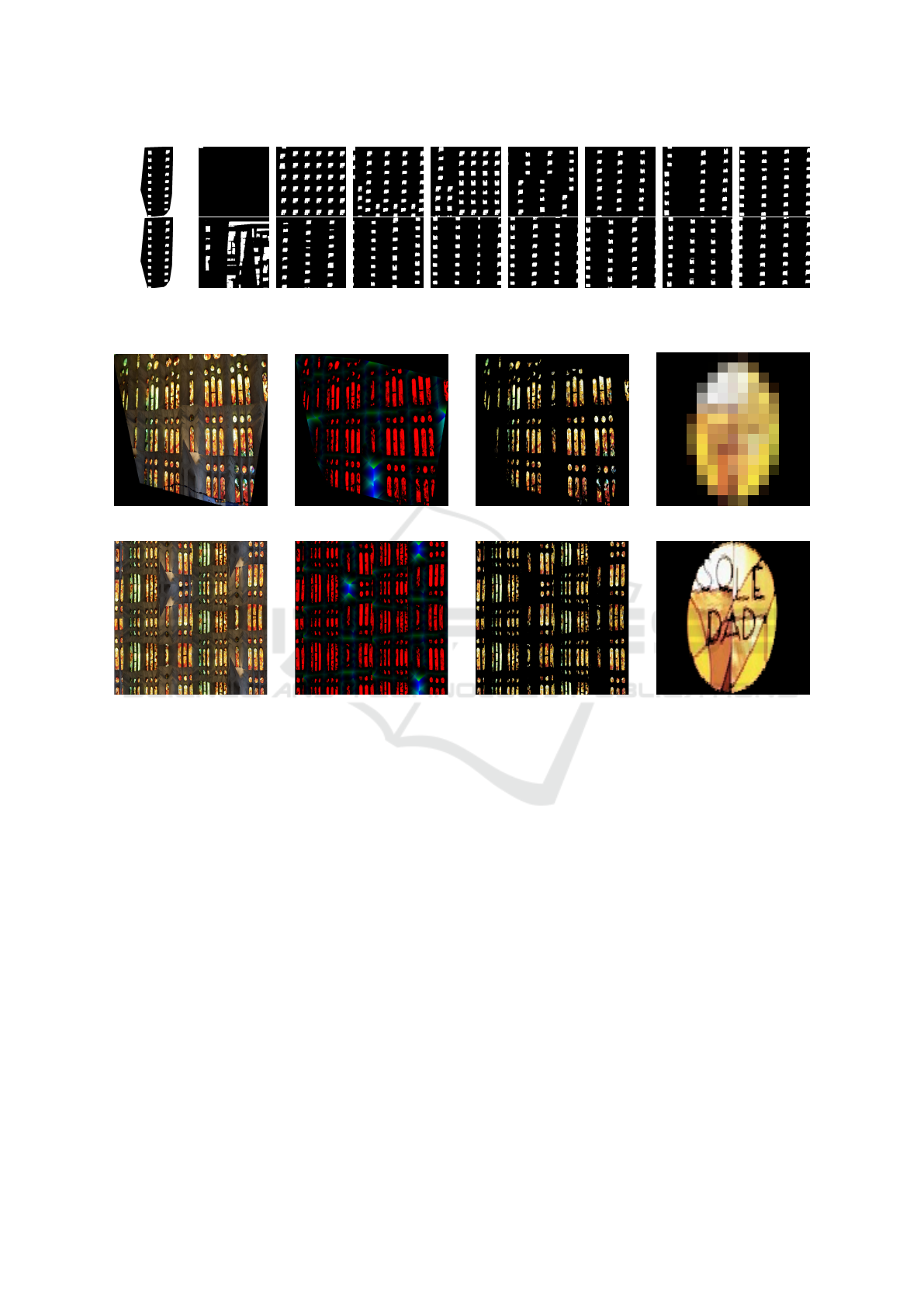
Figure 11: Comparison between direct texture synthesis (top row) and metadata-guided synthesis (bottom row). Including

additional spatial and application speciﬁc metadata in the synthesis process provides much more stable results. From left to

right: input, then results with block size varying from 25 pixels to 200 pixels in 25 pixels increases.

(a) Unwarped input (b) Input metadata (c) Emissive texture input (d) Down-scaled input

(e) Synthesized output (f) Output metadata (g) Emissive texture output (h) Recovered detail

Figure 12: Starting from the unwarped extraction of the input image (a), we perform texture synthesis using (b) metadata

(red: segmentation conﬁdence, green and blue: x and y distance to the nearest feature) and the selected lights (c) as input.

For additional speed-up, synthesis operates on a down-scaled version of this input data (d), and produces output data (e) and

metadata (f), which deﬁnes the emissive texture (g). We recover full-resolution details in a post-processing step (h).

7 PARAMETER OPTIMIZATION

Finally, for rendering purposes, we apply the synthe-

sized high-quality texture as an emissive texture on

a user-speciﬁed surface of the 3D scene. However,

while texture synthesis copies the shape and arrange-

ment of the light sources to the target scene, the ac-

tual appearance of the lighting can still differ from

the input. As illustrated in the middle row of Fig. 13,

a bright white light does not accurately recreate the

mood conveyed by the original image. The global il-

lumination of the scene also heavily depends on the

size of the light sources relative to the target scene.

To account for these effects, we perform a ﬁnal op-

timization step on the overall colour and intensity of

the emissive texture.

We extract the main colour of the user-selected

surface in the input image excluding light sources.

That is, we compute the average colour of the pix-

els corresponding to the selected surface but not to

light sources on this surface. This approach reduces

the possibility of unrelated objects in the scene af-

fecting the colour of the lighting. We set the target

illumination in the 3D scene, on the same surface

where the emissive texture is applied to this colour

(see Fig. 13, top right). Using a view-independent

framework based on differentiable rendering (Lipp

et al., 2024), we optimize the colour and intensity of

the emissive texture such that the light incident to the

same surface matches the target. Differentiable ren-

dering allows for efﬁcient gradient-based optimiza-

tion of the parameters. Because the target is collo-

Single-Exemplar Lighting Style Transfer via Emissive Texture Synthesis and Optimization

121

Figure 13: Output rendering and optimization. Top row:

original image and target ceiling colour. Middle row: ren-

dering of the initial state white light and arbitrary intensity.

Bottom row: optimized light colour and intensity. The right

column shows the corresponding simpliﬁed view used in-

ternally by the optimization framework.

cated with the light source, contributions to the illu-

mination of this surface arise either from the emis-

sive texture itself in the case of a concave surface,

or from indirect illumination scattered back from the

scene. This causes the colour of objects in the scene

to also be reﬂected in the ﬁnal colour and intensity of

the light source in order to provide the same overall

impression as the original image. Figure 13 (bottom

row) shows how the 3D scene looks after optimiza-

tion, with the left and right view corresponding to the

ﬁnal rendered image and the simpliﬁed model used

for optimization, respectively.

8 RESULTS

Figures 16 and 17 summarize results generated with

our system and compare to two general-purpose neu-

ral style transfer methods: (Gatys et al., 2015) and (Li

et al., 2018). The input images are shown on the left,

and each input is applied to two different 3D scenes: a

large living room (Fig. 16) and a smaller ofﬁce space

(Fig. 17). Because interpreting the quality of a light-

ing design is a deeply subjective matter, providing a

numeric validation of our result according to a pre-

cise metric is a difﬁcult task. We instead focus on a

qualitative analysis of the results to showcase how dif-

ferent aspects of the initial lighting conﬁgurations are

successfully reproduced in our examples, as well as

a user study to quantify the perception of our results

compared to other transfer methods.

8.1 Qualitative Validation

As we can see in Fig. 16 and 17, using different

input images drastically changes the appearance of

the generated lighting in the 3D scene. The overall

impression of each image is replicated through light

colour and intensity optimization (brightly lit for the

ﬁrst two, dimly lit for the following two, with dif-

ferent colour temperatures for each). Note that, the

shape of the light sources conveys different meanings

to the scene they illuminate (for example between the

well-spaced round lights of a lounge in the ﬁrst im-

age, a tight grid of square and round ofﬁce lights in

the second image, and the stained glass of a church

in the fourth). The effect of the optimization pro-

cess is particularly visible on the results obtained in

Fig. 16. Indeed, the red curtain and the ﬂoor, which

has a wooden material, naturally impact the colour

of the light as it is reﬂected. As a result, the inter-

action of a white light with the ﬂoor would produce

a more reddish tint than what would be expected, as

shown in the ﬁfth example. Our optimization auto-

matically compensates by adjusting the colour of the

light to a blue tint, thus keeping the colour of the ceil-

ing and overall scene close to the input image. This

effect can be observed on the back wall, where the

blue tint is particularly visible in the second example.

In contrast, the back wall stays grey in the last exam-

ple, as the colours of the input image already match

the wooden ﬂoor.

In comparison, these effects are not visible in any

of the neural style transfer methods, since they only

operate on images and do not take physical light trans-

port into account. These methods only copy the gen-

eral colour palette of the input image without having

access to semantic information about the nature of the

light or objects. As a result, unexpected artifacts are

visible in many of the results produced by the neu-

ral style transfer methods. For example, Fast Photo

Style (Li et al., 2018), produces blue highlights due

to the blue chairs in the lounge scene, and a glowing

curtain (in Fig. 16) and plant (in Fig. 17) in the church

example. The neural style transfer methods achieve

better results the more uniform the input example is,

which is most noticeable in examples 2 and 3.

8.2 User Study

We conducted an online user study via a self-hosted

webform. For all statistical tests, we use the stan-

dard α = 0.05 and, in case of multiple testing, report

GRAPP 2025 - 20th International Conference on Computer Graphics Theory and Applications

122

100

Very

Poor

Fair

Good

Very

Good

Very

Poor

Fair

Good

Very

Good

Count

FPhS

Ours

Comparison Scene 1: Stage

100

Count

Input Image: Museum

Church Office Reception Meeting

Comparison Scene 2: Office Room

FPhS

Ours

Very

Poor

Fair

Good

Very

Good

Very

Poor

Fair

Good

Very

Good

Very

Poor

Fair

Good

Very

Good

Very

Poor

Fair

Good

Very

Good

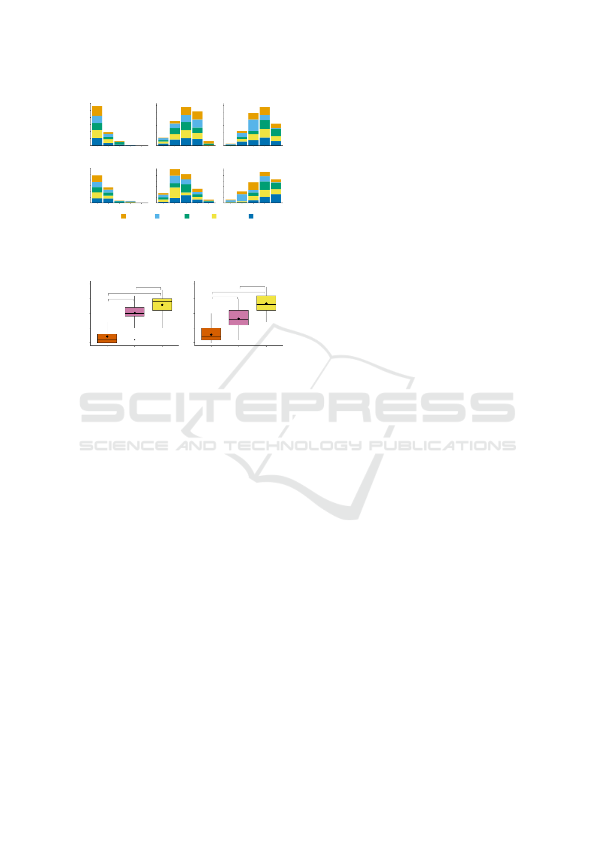
Figure 14: Barplot of the rating results by scene and input

image. Our method is consistently rated higher than previ-

ous work. ‘ST’: Style Transfer (Gatys et al., 2015), ‘FPhS’:

Fast Photo Style (Li et al., 2018).

****

FPhS

Ours ST

FPhS

Ours

Average Rating

Scene 1: Stage

****

−2

−1

−2

−1

Average Rating

Scene 2: Office Room

Figure 15: Boxplot of the rating results averaged across

all ﬁve input image scenarios (♦ mean, • weak outlier).

Statistically signiﬁcant relations according to pairwise,

Bonferroni-corrected paired Wilcoxon signed-rank tests are

connected on top, where the number of stars indicates the

signiﬁcance level (**: p < 0.01, ****: p < 0.0001).

adjusted p-values after applying Bonferroni correc-

tion for better readability. As effect sizes we report

Kendall’s W and Wilcoxon’s r (< 0.3 small, 0.3−0.5

moderate, > 0.5 large).

After participants agreed to our consent form, we

displayed a tutorial section explaining the theoreti-

cal context via exemplary line-art images of a refer-

ence with yellow light and two possible outcomes,

one with blue light (labelled wrong) and one with yel-

low light (labelled correct). The reference had small,

round lighting ﬁxtures on the ceiling, the ﬁrst re-

sult with blue lights large, rectangular ones, and the

yellow-coloured result no light ﬁxtures at all, so as

not to bias the participants towards our method. Af-

terwards, as an attention question, we displayed the

same line-art images again and asked which image

captures the lighting setup more accurately.

In the main body of the survey, participants ﬁrst

had to compare our method against results from style

transfer (ST) (Gatys et al., 2015) and Fast Photo Style

(FPhS) (Li et al., 2018) with ﬁve different input im-

ages applied to two target 3D scenes, resulting in the

ten scenarios shown in Fig. 16 (Scene 1: Stage) and

Fig. 17 (Scene 2: Ofﬁce Room). The order of the

scenes was ﬁxed, but the order of the different in-

put image scenarios was randomized for each par-

ticipant. Within each input image scenario, the or-

der of the methods was ﬁxed for all participants, but

varied between different input images. For each re-

sult image, participants were asked to rate on a ﬁve-

point labelled scale how well it represents how the

lighting of the reference image would look like in

the given 3D scene. Next, we showed them three

ﬂavours of our method (before optimization, and op-

timizing wrt. ceiling colour or overall colour) applied

to three different combinations of input image and 3D

scene and asked them to choose their favourite. While

we used the ceiling colour by default in our results,

we also presented optimization based on the average

colour of the whole image as an alternative since it

includes more information about the input.

Overall, we collected 38 submissions. After ﬁlter-

ing out four participants who answered the attention

question wrongly and one who stated an unrealistic

age of 99, we end up with a study population of N =

33 (female = 13, male = 16, diverse = 4), where the

participants’ age ranged from 21 to 60 (mean = 33.5,

std. dev. = 14.4). When asked about their main area

of expertise, two stated “art”, 18 “computer graphics”

and 13 “other”. 20 participants indicated they regu-

larly work with digital 3D models or scene represen-

tations (including renderings thereof) and 16 partici-

pants afﬁrmed that lighting plays an important role in

their professional or amateur work.

The rating results for each combination of a 3D

scene, input image and method are shown in Fig. 14.

While ST consistently was rated as mostly ‘Very

Poor’, FPhS achieved slightly better ratings in Scene

1 (mode = ‘Fair’) than in Scene 2 (mode = ‘Poor’).

For our method (both scenes: mode = ‘Good’), the

church input image for Scene 2 received the low-

est rating (mode = ‘Poor’), whereas the meeting

room image for Scene 2 received the highest rating

(mode = ‘Very Good’). To test the hypothesis that our

method is rated as better at representing the light setup

of a reference image in a 3D scene, we converted the

ratings to a zero-centred, numerical scale and for each

scene averaged the results across all ﬁve input im-

ages. As Shapiro-Wilk tests show a violated normal-

ity assumption, we apply a Friedmann test (the non-

parametric alternative to a one-way repeated mea-

sures ANOVA) to examine the differences between

the methods’ average ratings. For both scenes we ﬁnd

signiﬁcant differences with large effect sizes (Scene

1: χ

(2) = 44.4, p = 2e-10, W = .673; Scene 2:

(2) = 51.3, p = 7e-12, W = .777). To further inves-

tigate this, we conduct paired Wilcoxon signed-rank

tests (see Fig. 15). The highest p-value was found be-

tween our method and FPhS for scene 1 (p = 0.006,

r = 0.527), for all other combinations: p < 1e-5 and

Single-Exemplar Lighting Style Transfer via Emissive Texture Synthesis and Optimization

123

Inputs42

Method

Style transfer

(Gatys et al., 2015)

Fast Photo Style

(Li et al., 2018)

Ours

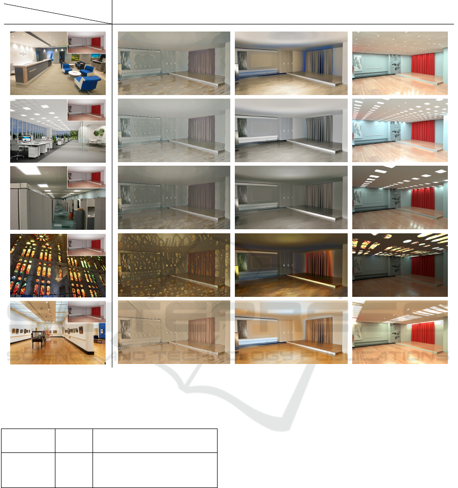
Figure 16: Table of results comparing our method to two deep-learning based general style transfer methods. The leftmost

column shows the different input images, as well as the 3D scene where the lighting is copied as an inset.

Table 1: Number of participants choosing a ﬂavour of our

method by input image and scene.

Input Scene

Before

Opt.

Ceiling

Colour

Overall

Colour

Ofﬁce Stage 3 13 17

Reception Stage 2 28 3

Church Ofﬁce 1 7 25

r > 0.764.

Regarding the ﬂavour of our method, there is

no clear winner between optimizing wrt. the ceiling

colour or overall colour as can be seen in Table 1. The

choice seems to be scene dependent and could thus be

left to the user as an adjustable parameter.

9 CONCLUSION

In this paper, we presented a novel copy-paste lighting

style transfer approach from a single image to a 3D

target scene. In contrast to machine-learning-based

solutions, our method allows for interactive control

by the user, and does not require specialized exper-

tise. Our results are physically plausible, as we simu-

late the full light transport in the 3D scene, contrary to

image-based methods. Our approach relies on a few

assumptions, which currently reduce the range of ad-

missible input images: light sources must be directly

visible, and sufﬁcient scene context is needed for the

perspective correction. We typically operate on inte-

riors, but images of exterior scenes satisfying these

criteria could also be used.

Using emissive textures as a way to encode and

copy the lighting conﬁguration of the input image

also incurs some limitations: lights are expected to

lie on or close to a surface for accurate modelling, as

hanging light ﬁxtures cannot be represented solely by

emissive textures.

Within these assumptions, however, our method

presents the ﬁrst interactive single-image, physically-

GRAPP 2025 - 20th International Conference on Computer Graphics Theory and Applications

124

Inputs42

Method

Style transfer

(Gatys et al., 2015)

Fast Photo Style

(Li et al., 2018)

Ours

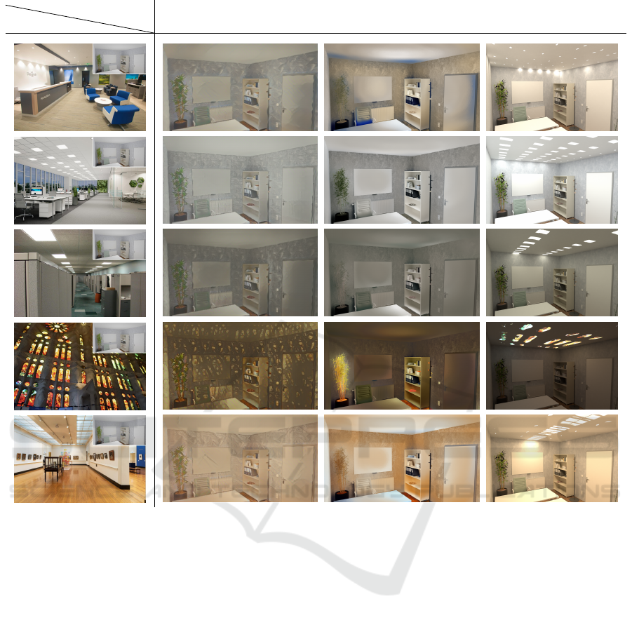
Figure 17: Similar table of results as Fig. 16, but applied to a 3D scene of a small ofﬁce.

based lighting style transfer method. We produce ex-

plainable and controllable results that can be gener-

ated by novice and expert users alike. Furthermore,

we show statistically signiﬁcant improvements in the

perceived quality of our lighting transfer compared to

image-based neural style transfer approaches.

In the future, we plan to extend our approach from

texture synthesis towards generating 3D geometry for

light ﬁxtures. Furthermore, allowing for multiple

lighting style images as inputs to produce a combi-

nation of these styles in the resulting 3D scene could

allow for more interactive exploration of the available

design space. We also envision a combination of our

method with other generative machine-learning ap-

proaches, or optimization-based methods, in order to

build a comprehensive digital lighting design toolkit.

ACKNOWLEDGEMENTS

This project has received funding from the Austrian

Science Fund (FWF) project F 77 (SFB “Advanced

Computational Design”).

REFERENCES

Anrys, F., Dutr

e, P., and Willems, Y. D. (2004). Image-

based lighting design. In Proc. 4th IASTED Interna-

tional Conference on Visualization, Imaging, and Im-

age Processing.

Canny, J. (1986). A computational approach to edge detec-

tion. Pattern Analysis and Machine Intelligence, IEEE

Transactions on, PAMI-8:679 – 698.

Chen, X., Jia, R., Ren, H., and Zhang, Y. (2010). A New

Vanishing Point Detection Algorithm Based on Hough

Transform. In 3rd International Joint Conference on

Computational Science and Optimization, volume 2,

pages 440–443.

Single-Exemplar Lighting Style Transfer via Emissive Texture Synthesis and Optimization

125

DIAL GmbH (2022). Dialux evo 10.1.

Diamanti, O., Barnes, C., Paris, S., Shechtman, E., and

Sorkine-Hornung, O. (2015). Synthesis of Complex

Image Appearance from Limited Exemplars. ACM

Transactions on Graphics, 34(2):1–14.

Duda, R. O. and Hart, P. E. (1972). Use of the hough trans-

formation to detect lines and curves in pictures. Com-

mun. ACM, 15(1):11–15.

Efros, A. A. and Freeman, W. T. (2001). Image quilting for

texture synthesis and transfer. In Proc. SIGGRAPH

’01, pages 341–346. ACM.

Efros, A. A. and Leung, T. K. (1999). Texture synthesis

by non-parametric sampling. In Proc. ICCV, pages

1033–1038. IEEE.

Eisenacher, C., Lefebvre, S., and Stamminger, M. (2008).

Texture Synthesis From Photographs. Computer

Graphics Forum, 27(2):419–428.

uhst

uck, A., Alhashim, I., and Wonka, P. (2019). Tile-

GAN: synthesis of large-scale non-homogeneous tex-

tures. ACM Transactions on Graphics, 38(4):1–11.

Gatys, L. A., Ecker, A. S., and Bethge, M. (2015). A neural

algorithm of artistic style. arXiv:1508.06576.

Gkaravelis, A. (2016). Inverse lighting design using a cov-

erage optimization strategy. The Visual Computer,

32(6):10.

Heitz, E., Vanhoey, K., Chambon, T., and Belcour, L.

(2021). A Sliced Wasserstein Loss for Neural Texture

Synthesis. In IEEE CVPR 2021, pages 9407–9415.

Jakob, W., Speierer, S., Roussel, N., Nimier-David, M.,

Vicini, D., Zeltner, T., Nicolet, B., Crespo, M.,

Leroy, V., and Zhang, Z. (2022). Mitsuba 3 renderer.

https://mitsuba-renderer.org.

Jin, S. and Lee, S.-H. (2019). Lighting Layout Optimization

for 3D Indoor Scenes. Computer Graphics Forum,

38(7):733–743.

Jing, Y., Yang, Y., Feng, Z., Ye, J., Yu, Y., and

Song, M. (2018). Neural style transfer: A review.

arXiv:1705.04058.

Kawai, J. K., Painter, J. S., and Cohen, M. F. (1993). Ra-

dioptimization: goal based rendering. In Proc. SIG-

GRAPH ’93, pages 147–154. ACM.

Kwatra, V., Essa, I., Bobick, A., and Kwatra, N. (2005).

Texture Optimization for Example-based Synthesis.

In Proc. SIGGRAPH ’05, pages 795–802.

Kwatra, V., Schodl, A., Essa, I., Turk, G., and Bobick, A.

(2003). Graphcut Textures: Image and Video Synthe-

sis Using Graph Cuts. In Proc. SIGGRAPH ’03, pages

277–286.

Lefebvre, S. and Hoppe, H. (2005). Parallel con-

trollable texture synthesis. ACM Trans. Graph.,

24(3):777–786.

Lefebvre, S. and Hoppe, H. (2006). Appearance-space tex-

ture synthesis. ACM Trans. Graph., 25(3):541–548.

Li, Y., Liu, M.-Y., Li, X., Yang, M.-H., and Kautz, J. (2018).

A closed-form solution to photorealistic image styl-

ization. arXiv:1802.06474.

Lin, W.-C., Huang, T.-S., Ho, T.-C., Chen, Y.-T., and

Chuang, J.-H. (2013). Interactive Lighting Design

with Hierarchical Light Representation. Computer

Graphics Forum, 32(4):133–142.

Lipp, L., Hahn, D., Ecormier-Nocca, P., Rist, F., and Wim-

mer, M. (2024). View-independent adjoint light trac-

ing for lighting design optimization. ACM Transac-

tions on Graphics, 43(3):1–16.

Liu, S., Zhou, Y., and Zhao, Y. (2021). VaPiD: A Rapid

Vanishing Point Detector via Learned Optimizers. In

Proc. ICCV 2021, pages 12839–12848.

Magee, M. and Aggarwal, J. (1984). Determining vanish-

ing points from perspective images. Computer Vision,

Graphics, and Image Processing, 26(2):256–267.

Okabe, M., Matsushita, Y., Shen, L., and Igarashi, T.

(2007). Illumination Brush: Interactive Design of All-

Frequency Lighting. In 15th Paciﬁc Conference on

Computer Graphics and Applications (PG’07), pages

171–180. IEEE.

Pellacini, F., Battaglia, F., Morley, R. K., and Finkelstein,

A. (2007). Lighting with paint. ACM Transactions on

Graphics, 26(2):9.

Ranftl, R., Lasinger, K., Hafner, D., Schindler, K., and

Koltun, V. (2022). Towards Robust Monocular Depth

Estimation: Mixing Datasets for Zero-Shot Cross-

Dataset Transfer. IEEE Trans. Pattern Anal. Mach.

Intell., 44(3):1623–1637.

Relux Informatik AG (2022). Reluxdesktop.

Ren, H., Fan, H., Wang, R., Huo, Y., Tang, R., Wang,

L., and Bao, H. (2023). Data-driven digital light-

ing design for residential indoor spaces. ACM Trans.

Graph., 42(3).

Risser, E. (2020). Optimal textures: Fast and robust texture

synthesis and style transfer through optimal transport.

CoRR, abs/2010.14702.

Schoeneman, C., Dorsey, J., Smits, B., Arvo, J., and Green-

berg, D. (1993). Painting with light. In Proc. SIG-

GRAPH ’93, pages 143–146. ACM.

Schwarz, M. and Wonka, P. (2014). Procedural Design of

Exterior Lighting for Buildings with Complex Con-

straints. ACM Transactions on Graphics, 33(5):1–16.

Sendik, O. and Cohen-Or, D. (2017). Deep correlations for

texture synthesis. ACM Trans. Graph., 36(5):1–15.

Sorger, J., Ortner, T., Luksch, C., Schw

arzler, M., Groller,

E., and Piringer, H. (2016). LiteVis: Integrated Vi-

sualization for Simulation-Based Decision Support in

Lighting Design. IEEE TVCG, 22(1):290–299.

Tong, X., Zhang, J., Liu, L., Wang, X., Guo, B., and

Shum, H.-Y. (2002). Synthesis of Bidirectional Tex-

ture Functions on Arbitrary Surfaces. In Proc. SIG-

GRAPH ’02, pages 665–672.

Walch, A., Schw

arzler, M., Luksch, C., Eisemann, E., and

Gschwandtner, T. (2019). LightGuider: Guiding In-

teractive Lighting Design using Suggestions, Prove-

nance, and Quality Visualization. IEEE TVCG.

Wu, J., Zhang, L., Liu, Y., and Chen, K. (2021).

Real-time vanishing point detector integrating under-

parameterized ransac and hough transform. In Proc.

ICCV 2021, pages 3732–3741.

Zhang, C., Miller, B., Yan, K., Gkioulekas, I., and Zhao,

S. (2020). Path-space differentiable rendering. ACM

Transactions on Graphics, 39(4).

Zhou, Q.-Y., Park, J., and Koltun, V. (2018a). Open3D:

A modern library for 3D data processing.

arXiv:1801.09847.

Zhou, Y., Zhu, Z., Bai, X., Lischinski, D., Cohen-Or, D.,

and Huang, H. (2018b). Non-Stationary Texture Syn-

thesis by Adversarial Expansion. arXiv:1805.04487.

GRAPP 2025 - 20th International Conference on Computer Graphics Theory and Applications

126